Core functionality
- The core module offers data structures and routines for creating and manipulating:
- geological description: structured and unstructured grids
- petrophysical properties (porosity, permeability, net to gross, etc)
- drive mechanisms (wells, boundary conditions)
- reservoir state (pressures, saturations, fluxes, etc.)
This includes, in particular, a large number of grid-factory routines and a routine for computing transmissibilities.
In addition, the core module provides:
- a library for automatic differentiation geared towards sparse matrices and coupled PDEs
- plotting of cell and face data defined over MRST grids
- physical units (length, time, mass, pressures, etc) and conversion routines
- basic reading, parsing, and writing ECLIPSE input data
- various utility routines and functionality
Plotting routines
A number of plotting routines are found as a part of MRST core. Different
routines allow for plotting of general unstructured grids, as well as data
located in cells, on faces or on nodes. For more interactive tools that build
upon this functionality, see the mrst-gui module.
-
Contents¶ - PLOTTING
- Routines for visual inspection of grid geometry and field properties.
- Files
- boundaryFaces - Extract boundary faces from set of grid cells. colorbarHist - Make colorbar with histogram on top outlineCoarseGrid - Impose outline of coarse grid on existing grid plot. plotBlockAndNeighbors - Plot a coarse block and its neighbours to current axes (reversed Z axis). plotCellData - Plot exterior grid faces, coloured by given data, to current axes. plotContours - Plot contours of cell data. plotFaceData - Plot face data on exterior grid faces to current axes (reversed Z axis). plotFaces - Plot selection of coloured grid faces to current axes (reversed Z axis). plotFaults - Plot faults in model plotGrid - Plot exterior faces of grid to current axes. plotGridVolumes - Plot partially transparent isosurfaces for a set of values plotNodeData - Plot data defined on nodes of grid plotSlice - Plot Cartesian slices of cell data on faces plotWell - Plot well trajectories into current axes.
-
boundaryFaces(g, varargin)¶ Extract boundary faces from set of grid cells.
Synopsis:
 f     = boundaryFaces(G)
 f     = boundaryFaces(G, cells)

[f, c] = boundaryFaces(...)
Parameters: - G – Grid data structure.
- cells – Non-empty subset of cells from which to extract boundary faces.
OPTIONAL. Default value:
cells = 1 : G.cells.num, meaning all external faces for all grid cells will be extracted. This amounts to extracting the entire boundary of ‘G’.
Returns: - f – List of faces bounding the sub domain given by
cells. - c – List of specific grid cells connected to the individual faces in
f. This may be useful for plotting cell data (e.g., the cell pressure) on the sub domain faces by means of functionplotFaces.
Example:
G    = cartGrid([40, 40, 5]);
rock = <some rock data structure for G>;

% 1) Plot (external) geometry of 'G'.
f  = boundaryFaces(G);
hg = plotFaces(G, f);

% 2) Plot horizontal permeability along diagonal of reservoir
[f, c] = boundaryFaces(G, 1 : G.cartDims(1) + 1 : G.cells.num);
hd     = plotFaces(G, f, log10(rock.perm(c,1)), 'FaceAlpha', 0.625);
See also
-
colorbarHist(q, lim, varargin)¶ Make colorbar with histogram on top
Synopsis:
colorbarHist(q, lim)
[hc,hh] = colorbarHist(q, lim, loc)
[hc,hh] = colorbarHist(q, lim, loc, n)
[hc,hh] = colorbarHist(q, lim, loc, n, islog)
Parameters: - q – vector for which histogram is to be defined
- lim – defines the range of values used to set limits of colorbar and axis of histogram for q
- loc – location of colorbar:
East,West, orSouth(default) - n – number of bins in histogram (default: 50). See the documentation of hist for the interpretation of this parameter.
- islog – flag indicating that we should visualize q on a logarithmic scale
Returns: - hc – graphics handle to colorbar
- hh – graphics handle to histogram
See also
hist
-
mrstColorbar(varargin)¶ Append a colorbar with an accompanying histogram to the current axis
Synopsis:
mrstColorbar
mrstColorbar(ax)
mrstColorbar(..,values)
[hc,hh] = mrstColorbar(..,location)
[hc,hh] = mrstColorbar(..,location, logscale)
[hc,hh] = mrstColorbar(..,location, logscale, limits)
Parameters: - ax – add colorbar to axes AX instead of current axis
- values – create the accompanying histogram using the VALUES vector. If not specified, the routine will pick values from CData of the current axes. Notice that many 3D plots in MRST only show the outer surface of a grid and hence the histogram will not represent the full 3D dataset unless this is explicitly specified.
- location – location of colorbar, same as for MATLAB’s colorbar except that the colorbar is always placed outside of the plot
- logscale – flag indicating that the data displayed are shown on a logarithmic scale. This will manipulate the the tick marks on the colorbar so that they are given in scientific notation
- limits – lower and upper limits for the histogram bins. NB! Setting this parameter will also reset the caxis accordingly.
Returns: - hc – graphics handle to colorbar
- hh – graphics handle to histogram
See also
hist
-
outlineCoarseGrid(G, p, varargin)¶ Impose outline of coarse grid on existing grid plot.
Synopsis:
 outlineCoarseGrid(G, p)
 outlineCoarseGrid(G, p, 'pn1', pv1, ...)
 outlineCoarseGrid(G, p, c, 'pn1', 'pv1', ...)

h = outlineCoarseGrid(...)
Parameters: - G – Grid data structure.
- p – Coarse grid partition vector as defined by (e.g) partitionUI and processPartition.
- c – color, works only if G.griddim==2
Keyword Arguments: ‘Any’ – Additional keyword arguments will be passed directly on to function
patchmeaning all properties supported bypatchare valid.Returns: h – Handle to polygonal patch structure as defined by function plotFaces. Only returned if requested.
Example:
G  = cartGrid([8, 8, 2]);
p  = partitionUI(G, [2, 2, 1]);
% plot fine grid:
plotGrid(G, 'faceColor', 'none'); view(3);
% outline coarse grid on fine grid:
outlineCoarseGrid(G, p);
-
plotBlockAndNeighbors(CG, block, varargin)¶ Plot a coarse block and its neighbours to current axes (reversed Z axis).
Different colours and levels of transparency are used to distinguish the blocks. The block itself is plotted in blue colour and the neighbours using colours from a brightened COLORCUBE colour map. Faults are plotted using gray patches (RGB = REPMAT(0.7, [1, 3])) with red edge colours.
Synopsis:
 plotBlockAndNeighbors(CG, block)
 plotBlockAndNeighbors(CG, block, 'pn1', 'pv1', ...)

h = plotBlockAndNeighbors(...)
Parameters: - CG – Coarse grid data structure.
- block – The coarse block to be plotted.
Keyword Arguments: PlotFaults – Two-element
logicalvector, the entries of which specify whether or not fault faces should be added to the graphical output of the ‘block’ and its neighbours, respectively.DEFAULT:
PlotFaults = TRUE([1,2])(attach fault faces to both the ‘block’ and all of its neighbours).Alpha –
(2 + max(find(PlotFaults)))-element numeric vector, values in [0,1], specifying scalar transparency (AlphaData) values for theblock, its neighbours, and the fault faces of the ‘block’ and its neighbours, respectively.DEFAULT:
Alpha = ONES([1,4])(no transparency in any of the final objects–all objects drawn opaquely).‘Any’ – Additional keyword arguments will be passed directly on to function
patchmeaning all properties supported bypatchare valid.
Returns: h – Handle to resulting patch objects. The patch objects are added directly to the current
axesobject (gca). OPTIONAL. Only returned if specifically requested.Example:
% Plot a block and its neighbours from a coarse partitioning of the
% "model 3" synthetic geometry
require coarsegrid  %  Make "coarse block" concept meaningful

% Generate geometry
G = processGRDECL(makeModel3([100, 60, 15]));

% Partition geometry
p = partitionUI(G, [ 5, 5, 3 ]);
p = compressPartition(processPartition(G, p));

% Generate coarse grid
CG = generateCoarseGrid(G, p);

% Plot selected block (# 37) and its neighbours
plotBlockAndNeighbors(CG, 37, 'Alpha', repmat(0.75, [1, 4]))
view(-145, 26)
Notes
Function
plotBlockAndNeighborsis implemented in terms of plotting functionplotFaceswhich in turn uses the built-in functionpatch. If a separate axes is needed for the graphical output, callers should employ functionnewplotprior to callingplotBlockAndNeighbors. This function relies on a specific set of values for the propertiesFaceColorandFaceAlpha.See also
plotFaces,patch,newplot
-
plotCellData(G, data, varargin)¶ Plot exterior grid faces, coloured by given data, to current axes.
Synopsis:
 plotCellData(G, data)
 plotCellData(G, data, 'pn1', pv1, ...)
 plotCellData(G, data, cells)
 plotCellData(G, data, cells, 'pn1', pv1, ...)

h = plotCellData(...)
Parameters: - G – Grid data structure.
- data – Scalar cell data with which to colour the grid. One scalar, indexed colour value for each cell in the grid or one TrueColor value for each cell. If a cell subset is specified in terms of the ‘cells’ parameter, ‘data’ must either contain one scalar value for each cell in the model or one scalar value for each cell in this subset.
- cells –
Vector of cell indices defining sub grid. The graphical output of function ‘plotCellData’ will be restricted to the subset of cells from ‘G’ represented by ‘cells’.
If unspecified, function ‘plotCellData’ will behave as if the user defined
cells = 1 : G.cells.nummeaning graphical output will be produced for all cells in the grid model
G. Ifcellsis empty (i.e., ifisempty(cells)), then no graphical output will be produced.
Keyword Arguments: ‘Any’ – Additional keyword arguments will be passed directly on to function
patchmeaning all properties supported bypatchare valid.Returns: h – Handle to resulting patch object. The patch object is added directly to the current
axesobject (gca). OPTIONAL. Only returned if specifically requested. Ifisempty(cells), thenh==-1.Notes
Function
plotCellDatais implemented directly in terms of the low-level functionpatch. If a separate axes is needed for the graphical output, callers should employ functionnewplotprior to callingplotCellData.Example:
% Given a grid 'G' and a reservoir solution structure 'resSol' returned
% from, e.g., function 'solveIncompFlow', plot the cell pressure in bar:

   figure, plotCellData(G, convertTo(resSol.pressure, barsa()));
See also
plotFaces,boundaryFaces,patch,newplot
-
plotContours(g, value, n)¶ Plot contours of cell data.
Synopsis:
plotContours(G, field, n)
Description:
Function ‘plotContours’ is a poor-man’s implementation of the contour-level drawing function
contourfdesigned to work with MRST’s grid structure and cell-based values rather than the pure Cartesian (tensor product) nodal values ofcontourf. The contour lines follow the grid lines and are, typically, not smooth.The MRST function
plotGridVolumes, which interpolates the data field onto a structured grid, is an alternative option for visualising levels and iso-surfaces.Parameters: - G – Grid structure.
- field – Scalar field (e.g., cell pressures). Used as value data for determining the contour locations. One scalar value for each cell in ‘G’.
- n – Number of (equidistant) contour lines/levels for
field. Positive integer.
Returns: Nothing.
Example:
% Visualise the iso-levels of the pressure field of a quarter five-spot
% configuration.  Note that the actual pressure values in this case are
% artificial due to (very) high permeabilities (approximately 1e+12 D).
%
G     = computeGeometry(cartGrid([50, 50, 1]));
rock  = struct('perm', ones([G.cells.num, 1]));
T     = computeTrans(G, rock);
fluid = initSingleFluid('mu', 1, 'rho', 0);
src   = addSource([], [1, G.cells.num], [1, -1]);
x     = initState(G, [], 0);
x     = incompTPFA(x, G, T, fluid, 'src', src);

plotContours(G, x.pressure, 20), axis equal tight
Note
Function
plotContoursis only supported in three space dimensions i.e., ifG.griddim == 3.See also
plotGridVolumes,plotCellData,plotFaces,contourf
-
plotFaceData(G, varargin)¶ Plot face data on exterior grid faces to current axes (reversed Z axis).
Synopsis:
 plotFaceData(G, data)
 plotFaceData(G, data, 'pn1', pv1, ...)
 plotFaceData(G, cells, data)
 plotFaceData(G, cells, data, 'pn1', pv1, ...)

h = plotFaceData(...)
Parameters: - G – Grid data structure.
- data – Vector of values for each face in G.
- cells –
Vector of cell indices defining sub grid.
If unspecified, function
plotFaceDatawill behave as if the caller definedcells = 1 : G.cells.nummeaning graphical output will be produced for all cells in the grid model
G. Ifcellsis empty (i.e., ifisempty(cells)), then no graphical output will be produced.
Keyword Arguments: ‘Any’ – Additional keyword arguments will be passed directly on to function
patchmeaning all properties supported bypatchare valid.Returns: h – Handle to resulting patch object. The patch object is added directly to the current
axesobject (gca). OPTIONAL. Only returned if specifically requested. Ifisempty(cells), thenh==-1.See also
plotCellData,plotFaces,patch,newplot
-
plotFaces(G, varargin)¶ Plot selection of coloured grid faces to current axes (reversed Z axis).
Synopsis:
 plotFaces(G, faces)
 plotFaces(G, faces, 'pn1', pv1, ...)
 plotFaces(G, faces, colour)
 plotFaces(G, faces, colour, 'pn1', pv1, ...)

h = plotFaces(...)
Parameters: - G – Grid data structure.
- faces – Vector of face indices or a logical vector of length
G.faces.num. The graphical output of
plotFaceswill be restricted to the subset of grid faces fromGrepresented byfaces. - colour –
Colour data specification. Either a MATLAB
ColorSpec(i.e., an RGB triplet (1-by-3 row vector) or a short or long colour name such as ‘r’ or ‘cyan’), or apatchFaceVertexCDatatable suitable for either indexed or ‘true-colour’ face colouring. This data MUST be an m-by-1 column vector or an m-by-3 matrix. We assume the following conventions for the size of the colour data:any(size(colour,1) == [1, numel(faces)])One (constant) indexed colour for each face infaces. This option supportsflatface shading only. Ifsize(colour,1) == 1, then the same colour is used for all faces infaces.size(colour,1) == G.nodes.numOne (constant) indexed colour for each node infaces. This option must be chosen in order to support interpolated face shading.
OPTIONAL. Default value:
colour = 'y'(shading flat).
Keyword Arguments: - ‘Any ‘ – Additional keyword arguments will be passed directly on to
function
patchmeaning all properties supported bypatchare valid. - ‘Outline’ – Boolean option. When enabled,
plotFacesdraws the outline edge of thefacesinput argument. The outline is defined as those edges that appear exactly once in the edge list implied byfaces.
Returns: h – Handle to resulting
patchobject. The patch object is added to the currentaxesobject.Notes
Function
plotFacesis implemented directly in terms of the low-level functionpatch. If a separate axes is needed for the graphical output, callers should employ functionnewplotprior to callingplotFaces.Example:
% Plot grid with boundary faces on left side in red colour:
G     = cartGrid([5, 5, 2]);
faces = boundaryFaceIndices(G, 'LEFT', 1:5, 1:2, []);
plotGrid (G, 'faceColor', 'none'); view(3)
plotFaces(G, faces, 'r');
See also
plotCellData,plotGrid,newplot,patch,shading
-
plotFaults(G, faults, varargin)¶ Plot faults in model
Synopsis:
plotFaults(G, faults)
h = plotFaults(G, faults)
Parameters: - G – Valid grid structure.
- faults – Valid fault structure as defined by function
processFaults.
Returns: h – Two-element cell array of handles suitable for passing to
getorset. Specifically,h{1}is apatchhandle to the set of graphics containing the fault faces whileh{2}is a set oftexthandles to the corresponding fault names.OPTIONAL. Only returned if specifically requested.
See also
plotFaces,patch,text
-
plotGrid(G, varargin)¶ Plot exterior faces of grid to current axes.
Synopsis:
 plotGrid(G)
 plotGrid(G, 'pn1', pv1, ...)
 plotGrid(G, cells)
 plotGrid(G, cells, 'pn1', pv1, ...)

h = plotGrid(...)
Parameters: - G – Grid data structure.
- cells –
Vector of cell indices defining sub grid. The graphical output of function
plotGridwill be restricted to the subset of cells fromGrepresented bycells.If unspecified, function
plotGridwill behave as if the caller definedcells = 1 : G.cells.nummeaning graphical output will be produced for all cells in the grid model
G. Ifcellsis empty (i.e., ifisempty(cells)), then no graphical output will be produced.
Keyword Arguments: ‘Any’ – Additional keyword arguments will be passed directly on to function
patchmeaning all properties supported bypatchare valid.Returns: h – Handle to resulting patch object. The patch object is added directly to the current
axesobject (gca). OPTIONAL. Only returned if specifically requested. Ifisempty(cells), thenh==-1.Notes
Function
plotGridis implemented directly in terms of the low-level functionpatch. If a separate axes is needed for the graphical output, callers should employ functionnewplotprior to callingplotGrid.Example:
G = cartGrid([10, 10, 5]);

% 1) Plot grid with yellow colour on faces (default):
figure, plotGrid(G, 'EdgeAlpha', 0.1); view(3)

% 2) Plot grid with no colour on faces (transparent faces):
figure, plotGrid(G, 'FaceColor', 'none'); view(3)
See also
plotCellData,plotFaces,patch,newplot
-
plotGridVolumes(G, values, varargin)¶ Plot partially transparent isosurfaces for a set of values
Synopsis:
plotGridVolumes(G, data)
plotGridVolumes(G, data, 'pn', pv,...)
interpolant = plotGridVolumes(...)
Parameters: - G – Grid data structure
- values – A list of values to be plotted
Keyword Arguments: - ‘N’ – The number of bins used to create the isosurfaces.
- ‘min’ – Minimum value to plot. This is useful to create plots where high values are visible.
- ‘max’ – Maximum value to plot.
- ‘mesh’ – The mesh size used to sample the interpolant. Should be a row vector of length 3. Defaults to G.cartDims.
- ‘cmap’ – Function handle to colormap function. Using different colormaps for different datasets makes it possible to create fairly complex visualizations.
- ‘basealpha’ – Set to a value lower than 1 to increase transparency, set it to a larger value to decrease transparency.
- ‘binc’ – Do not call hist on dataset. Instead, use provided bins. To get good results, do not call binc option with unique(data): Ideally, binc’s values should be between the unique values.
- ‘patchn’ – Maximum number of patch faces in total for one call of plotGridVolumes. If this number is large, the process may be computationally intensive.
- ‘interpolant’ – If you are plotting the same dataset many times, the interpolant can be returned and stored.
- ‘extrudefaces’ – Let the cell values be extrapolated to the edges of the domain. Turn this off if you get strange results.
Returns: interpolant – See keyword argument of same name.
See also
-
plotNodeData(G, node_data, varargin)¶ Plot data defined on nodes of grid
Synopsis:
plotNodeData(G, data)
Parameters: - G – Grid data structure.
- node_data – Data at nodes to be plotted.
Keyword Arguments: ‘Any’ – Additional keyword arguments will be passed directly on to function
patchmeaning all properties supported bypatchare valid.Returns: h – Handle to resulting PATCH object. The patch object is added to the current AXES object.
Example:
G = cartGrid([10, 10]);
plotNodeData(G, G.nodes.coords(:, 1));
See also
plotCellData,plotGrid,newplot,patch,shading.
-
plotSlice(G, data_in, slice_ind, dim)¶ Plot Cartesian slices of cell data on faces
Synopsis:
h = plotSlice(G, data_inn, slice_ind, dim)
Parameters: - G – Grid data structure.
- data_in – Cell data to be plotted
- slice_ind – Index of slice
- dim – Dimension of slice
Returns: h – Handle to resulting
patchobject. The patch object is added to the currentaxesobject.
-
plotWell(G, W, varargin)¶ Plot well trajectories into current axes.
Synopsis:
[htop, htext, hs, hline] = plotWell(G, W)
[htop, htext, hs, hline] = plotWell(G, W, 'pn1', pv1, ...)
Parameters: - G – Grid data structure
- W – Well data structure
Keyword Arguments: - ‘radius’ – Scaling factor for the width of the well path. Default value: 1.0
- ‘height’ – Height above top reservoir contact at which the well should stop and symbol be drawn. Default value: height = 5
- ‘color’ – Colour with which the well path should be drawn. Possible
values described in
plot. Default value: color = ‘r’ - ‘color2’ – Second color. Will be used for producer wells. If not
specified, all wells will have the same color and the
colorargument will be used. - ‘cylpts’ – Number of segments to use about the well bore. A higher value produces more smoothly looking well trajectories at the expense of more costly plotting. Default value: cylpts = 10
- ‘fontsize’ – The size of the font used for the label texts. Default value: fontsize = 16
- ‘ambstr’ – The ambient strength of the well cylinder. Default value: ambstr = 0.8
- ‘linewidth’ – The width of the line above the well. Default value: linewidth = 2
Returns: - htop – Graphics handles to all well heads and heels.
- htext – Graphics handles to all rendered well names.
- hs – Graphics handles to all well paths.
- hline – Graphics handles to all lines between well head and names
Example:
G = computeGeometry(cartGrid([10, 1, 1]));
rock = makeRock(G, 1, 1);
W = addWell([], G, rock, 1)
plotWell(G, W, 'color', 'k');
Note
Currently, this function only supports three-dimensional grids.
See also
addWell,delete,patch,incompTutorialWells
Grid generation, processing and manipulation
-
Contents¶ - GRIDPROCESSING
- Construct and manipulate the MRST grid datastructures.
- Files
- buildCornerPtNodes - Construct physical nodal coordinates for CP grid.
buildCornerPtPillars - Construct physical nodal coordinates for CP grid.
cart2active - Compute active cell numbers from linear Cartesian index.
cartGrid - Construct 2d or 3d Cartesian grid in physical space.
cellNodes - Extract local-to-global vertex numbering for grid cells.
checkAndRepairZCORN - Detect and repair artifacts that may occur in corner-point specification.
computeGeometry - Add geometry information (centroids, volumes, areas) to a grid
extended_grid_structure - Extended grid structure
extractSubgrid - Construct valid grid definition from subset of existing grid cells.
glue2DGrid - Connect two 2D grids along common edge
grid_structure - Grid structure used in the MATLAB Reservoir Simulation Toolbox.
grdeclXYZ - Get corner-point pillars and coordinates in alternate format
hexahedralGrid - Construct valid grid definition from points and list of hexahedra
makeInternalBoundary - Make internal boundary in grid along specified faces.
makeLayeredGrid - Extrude 2D Grid to layered 3D grid with specified layering structure
pebi - Compute dual grid of triangular grid G.
processFaults - Construct fault structure from input specification (keyword
FAULTS) processGRDECL - Compute grid topology and geometry from pillar grid description. processNNC - Establish explicit non-neighbouring connections from NNC keyword processPINCH - Establish vertical non-neighbouring across pinched-out layers refineDeck - Refine the grid resolution of a deck, and update other information refineGrdecl - Refine an Eclipse grid (GRDECL file) with a specified factor in each of removeCells - Remove cells from grid and renumber cells, faces and nodes. removeFaultBdryFaces - Remove fault faces on boundary removeInternalBoundary - Remove internal boundary in grid by merging faces in face list N removeIntGrid - Cast any grid fields that are presently int32 to double removePinch - Uniquify nodes, remove pinched faces and cells. removeShortEdges - Replace short edges in grid G by a single node. splitDisconnectedGrid - Split grid into disconnected components tensorGrid - Construct Cartesian grid with variable physical cell sizes. tessellationGrid - Construct valid grid definition from points and tessellation list tetrahedralGrid - Construct valid grid definition from points and tetrahedron list triangleGrid - Construct valid grid definition from points and triangle list triangulateFaces - Split face f in grid G into subfaces.
-
buildCornerPtNodes(grdecl, varargin)¶ Construct physical nodal coordinates for CP grid.
Synopsis:
[X, Y, Z, lineIx] = buildCornerPtNodes(grdecl)
[X, Y, Z, lineIx] = buildCornerPtNodes(grdecl, 'pn1', pv1, ...)
Parameters: grdecl – Eclipse file output structure as defined by
readGRDECL. Must contain at least the fieldscartDims,COORDandZCORN.Keyword Arguments: - ‘Verbose’ – Whether or not to emit informational messages. Default value: Verbose = mrstVerbose.
- ‘CoincidenceTolerance’ – Absolute tolerance used to detect collapsed
pillars where the top pillar point coincides
with the bottom pillar point. Such pillars are
treated as is they were vertical.
Default value: CoincidenceTolerance =
100*eps.
Returns: - X, Y, Z – Size
2*grdecl.cartDimsarrays ofx,yandzphysical nodal coordinates, respectively. - lineIx – Index of pillar line. There are (nx+1)x(ny+1) pillar lines
along which node coordinates are defined by their
ZCORNvalue.
Example:
gridfile  = [DATADIR, filesep, 'case.grdecl'];
grdecl    = readGRDECL(gridfile);
[X, Y, Z] = buildCornerPtNodes(grdecl);
See also
-
buildCornerPtPillars(grdecl, varargin)¶ Construct physical nodal coordinates for CP grid.
Synopsis:
[X, Y, Z] = buildCornerPtPillars(grdecl)
[X, Y, Z] = buildCornerPtPillars(grdecl, 'pn1', pv1, ...)
Parameters: grdecl – Eclipse file output structure as defined by readGRDECL. Must contain at least the fields ‘cartDims’, ‘COORD’ and ‘ZCORN’.
Keyword Arguments: - ‘Verbose’ – Whether or not to emit informational messages. Default value: Verbose = mrstVerbose.
- ‘CoincidenceTolerance’ – Absolute tolerance used to detect collapsed
pillars where the top pillar point coincides
with the bottom pillar point. Such pillars are
treated as is they were vertical.
Default value: CoincidenceTolerance =
100*eps. - ‘Scale’ – Scale the pillars so that the extend from the top to the bottom of the model. Default: FALSE
Returns: X, Y, Z – Matrices with (nx+1)*(ny+1) rows with the start and end point of the pillars in ‘x’, ‘y’, and ‘z’ direction.
Example:
gridfile  = [DATADIR, filesep, 'case.grdecl'];
grdecl    = readGRDECL(gridfile);
[X, Y, Z] = buildCornerPtPillars(grdecl);
See also
-
cart2active(G, cartCells)¶ Compute active cell numbers from linear Cartesian index.
Synopsis:
activeCells = cart2active(G, c)
Parameters: - G – Grid data structure as described by
grid_structure. - c – List of linear Cartesian cell indices.
Returns: activeCells – Active cell numbers corresponding to the individual Cartesian cell numbers in
c.Note
This function provides the inverse mapping of the
G.cells.indexMapfield in the grid data structure.See also
- G – Grid data structure as described by
-
cartGrid(celldim, varargin)¶ Construct 2d or 3d Cartesian grid in physical space.
Synopsis:
G = cartGrid(celldim);
G = cartGrid(celldim, physdim);
Parameters: - celldim – Vector, length 2 or 3, specifying number of cells in each coordinate direction.
- physdim – Vector, length numel(celldim), of physical size in units of meters of the computational domain. OPTIONAL. Default value == celldim (i.e., each cell has physical dimension 1-by-1-by-1 m).
- cellnodes – OPTIONAL. Default value FALSE. If TRUE, the corner points of each cell is added as field G.cellNodes. The field has one row per cell, the sequence of nodes on each is (imin, jmin,kmin), (imax,jmin,kmin), (imin,jmax,kmin), …
Returns: G – Grid structure with a subset of the fields
grid_structure. Specifically, the geometry fields are missing:- G.cells.volumes
- G.cells.centroids
- G.faces.areas
- G.faces.normals
- G.faces.centroids
These fields may be computed using the function
computeGeometry.There is, however, an additional field not described in `grid_structure:
cartDimsis a length 2 or 3 vector giving number of cells in each coordinate direction. In other wordsall(G.cartDims == celldim).G.cells.faces(:,2)contains integers 1-6 corresponding to directions W, E, S, N, T, B respectively.Example:
% Make a 10-by-5-by-2 grid on the unit cube.
   nx = 10; ny = 5; nz = 2;
   G = cartGrid([nx, ny, nz], [1, 1, 1]);

% Plot the grid in 3D-view.
   f = plotGrid(G); view(3);
See also
-
cellNodes(g)¶ Extract local-to-global vertex numbering for grid cells.
Synopsis:
cn = cellNodes(G)
Parameters: G – Grid data structure geometrically discretising a reservoir model.
Returns: cn – An m-by-3 array mapping cell numbers to vertex numbers. Specifically, if
cn(i,1)==jandcn(i,3)==k, then global vertexkis one of the corners of cellj. The local vertex number of global nodekwithin celljmay be computed using the following statements:n_vert = accumarray(cn(:,1), 1, [G.cells.num, 1]); offset = rldecode(cumsum([0; n_vert(1:end-1)]), n_vert); loc_no = (1 : size(cn,1)).' - offset;
This calculation is only for illustration purposes. It is assumed that the local vertex number will be implicitly available in most applications (e.g., finite element methods).
Alternatively, the local vertex number is found in
cn(i,2). ;). In a corner-point grid, local vertex number of zero indicates that the vertex is not part of the original 8 vertices.See also
-
checkAndRepairZCORN(zcorn, cartDims, varargin)¶ Detect and repair artifacts that may occur in corner-point specification.
Synopsis:
zcorn = checkAndRepairZCORN(zcorn, dims)
zcorn = checkAndRepairZCORN(zcorn, dims, 'pn1', pv1, ...)
Description:
Function
checkAndRepairZCORNdetects and repairs the following, rare, conditions- Upper corners of a cell below lower corners of that same cell
- Lower corners of a cell below that cell’s lower neighbour’s upper corners.
These will typically arise as a result of finite precision output from a corner-point grid generator.
The repair strategy, if applicable, is as follows,
- If an upper corner is below the corresponding lower corner on the same pillar, then the upper corner depth is assigned to be equal to the lower corner depth.
- If a cell’s lower corner is below that cell’s lower neighbour’s upper corner on the same pillar, then the lower neighbour’s upper corner is assigned the corner depth of the upper cell’s lower corner.
Parameters: - zcorn – Corner-point depth specification of a corner-point grid. This value typically corresponds to the ‘ZCORN’ field of a data structure created by function ‘readGRDECL’.
- dims – Cartesian dimensions of the corner-point geometry. Assumed to be a three-element vector of (positive) extents. Typically corresponds to the field ‘cartDims’ of a ‘grdecl’ structure created by function ‘readGRDECL’.
Keyword Arguments: Active – A
prod(dims)-element vector of active cell mappings. Zero/false signifies inactive cells while non-zero/true signifies active cells. Typically corresponds to the fieldACTNUMof a ‘grdecl’ structure.Default value:
Active=[](-> All cells active).Verbose – Whether or not to emit informational messages during the computational process. Default value:
Verbose = mrstVerbose.
Returns: zcorn – Corner-point depth specification for which identified problems have been corrected. If there are no problems, then this is the same as input array ‘zcorn’.
Note
This function is used to implement option
RepairZCORNof the corner-point processor,processGRDECL.See also
-
computeGeometry(G, varargin)¶ Add geometry information (centroids, volumes, areas) to a grid
Synopsis:
G = computeGeometry(G)
G = computeGeometry(G, 'pn1', pv1, ...)
Parameters: G – Grid structure as described by grid_structure.
Keyword Arguments: ‘verbose’ – Whether or not to display informational messages during the computational process. Logical. Default value:
Verbose = mrstVerbose‘hingenodes’ – Structure with fields ‘faces’ and ‘nodes’. A hinge node is an extra center node for a face, that is used to triangulate the face geometry. For each face number F in ‘faces’ there is a row in ‘nodes’ which holds the node coordinate for the hinge node belonging to face F.
Default value: hingenodes = [] (no additional center nodes).
‘MaxBlockSize’ – Maximum number of grid cells to process in a single pass. Increasing this number may reduce overall computational time, but will increase total memory use. If empty (i.e., if
isempty(MaxBlockSize)istrue) or negative, process all grid cells in a single pass.Numeric scalar. Default value: MaxBlockSize = 20e3.
Returns: G – Grid structure with added fields:
cells
- volumes : A
G.cells.numby1array of cell volumes. - centroids: A
G.cells.numbysize(G.nodes.coords, 2)array of (approximate) cell centroids.
- volumes : A
faces
- areas: A
G.faces.numby1array of face areas. - normals: A
G.faces.numbyG.griddimarray of normals. - centroids: A
G.faces.numbysize(G.nodes.coords, 2)array of (approximate) face centroids.
- areas: A
Note
Individual face normals have length (i.e., Euclidian norm) equal to the corresponding face areas. In other words, subject to numerical round-off, the identity
norm(G.faces.normals(i,:), 2) == G.faces.areas(i)holds for all faces
i=1:G.faces.num.In three space dimensions, i.e., when
G.griddim == 3, function ‘computeGeometry’ assumes that the nodes on a given face,f, are ordered such that the face normal onfis directed from cellG.faces.neighbors(f,1)to cellG.faces.neighbors(f,2).See also
-
extended_grid_structure()¶ Extended grid structure
Synopsis:
Description of the grid structure with augmented mappings and
structures. In particular, topological description and geometrical
properties of the edges are included.  Such information is used in the VEM
assembly. Here, we describe the full structure. The structure that are added
with respect to grid_structure are marked as "(added structure)" or "(added
mapping)".
Returns: G – representation of grids on an unstructured format. A master
structure having the following fields –
- cells –
- A structure specifying properties for each individual cell in the grid. See CELLS below for details.
- faces –
- A structure specifying properties for each individual face in the grid. See FACES below for details.
- edges – (added structure)
- A structure specifying properties for each individual edge in the grid. See EDGES below for details.
- nodes –
- A structure specifying properties for each individual node (vertex) in the grid. See NODES below for details.
- type –
- A cell array of strings describing the history of grid constructor and modifier functions through which a particular grid structure has been defined.
- griddim –
- The dimension of the grid which in most cases will equal size(G.nodes.coords,2).
CELLS – Cell structure G.cells: - num –
Number of cells in the global grid.
- facePos –
Indirection map of size [num+1,1] into the ‘cells.faces’ array. Specifically, the face information of cell ‘i’ is found in the submatrix
G.cells.faces(facePos(i) : facePos(i+1)-1, :)
The number of faces of each cell may be computed using the statement DIFF(facePos).
- faces –
A (G.cells.facePos(end)-1)-by-2 array of global faces connected to a given cell. Specifically, if ‘cells.faces(i,1)==j’, then global face ‘cells.faces(i,2)’ is connected to global cell `j’.
To conserve memory, only the second column is actually stored in the grid structure. The first column may be re-constructed using the statement
- rldecode(1 : G.cells.num, …
diff(G.cells.facePos), 2) .’
A grid constructor may, optionally, append a third column to this array. In this case ‘cells.faces(i,3)’ often contains a tag by which the cardinal direction of face ‘cells.faces(i,2)’ within cell ‘cells.faces(i,1)’ may be distinguished. Some ancillary utilities within the toolbox depend on this specific semantics of ‘cells.faces(i,3)’, e.g., to easily specify boundary conditions (functions ‘pside’ and ‘fluxside’).
- nodePos – (added mapping)
Indirection map of size [num+1,1] into the ‘cells.nodes’ array. Specifically, the face information of cell ‘i’ is found in the submatrix
G.cells.nodes(nodePos(i) : nodePos(i+1)-1, :)
The number of nodes of each cell may be computed using the statement DIFF(nodePos).
- nodes – (added mapping)
A (G.cells.nodePos(end)-1)-by-2 array of global nodes belonging to a given cell. Specifically, if ‘cells.nodes(i,1)==j’, then global node ‘cells.nodes(i,2)’ is connected to global cell `j’.
To conserve memory, only the second column is actually stored in the grid structure. The first column may be re-constructed using the statement
- rldecode(1 : G.cells.num, …
diff(G.cells.nodePos), 2) .’
- indexMap –
Maps internal to external grid cells (i.e., active cell numbers to global cell numbers). In the case of Cartesian grids, indexMap == (1 : G.cells.num)’ .
For grids with a logically Cartesian topology of dimension ‘dims’ (a curvilinear grid, a corner-point grid, etc), a map of cell numbers to logical indices may be constructed using the following statement in 2D
[ij{1:2}] = ind2sub(dims, G.cells.indexMap(:)); ij = [ij{:}];
and likewise in 3D
[ijk{1:3}] = ind2sub(dims, G.cells.indexMap(:)); ijk = [ijk{:}];
In the latter case, ijk(i,:) is global (I,J,K) index of cell ‘i’.
- volumes –
A G.cells.num-by-1 array of cell volumes.
- centroids –
A G.cells.num-by-d array of cell centroids in R^d.
FACES – Face structure G.faces: - num –
Number of global faces in grid.
- edgePos – (added mapping)
Indirection map of size [num+1,1] into the ‘face.edges’ array. Specifically, the edge information of face ‘i’ is found in the submatrix
G.faces.edges(edgePos(i) : edgePos(i+1)-1, :)
The number of edges of each face may be computed using the statement DIFF(edgePos).
- edges – (added mapping)
A (G.faces.edgePos(end)-1)-by-2 array of vertices in the grid. Specifically, if ‘faces.edges(i,1)==j’, then global edge ‘faces.edges(i,2)’ is part of the global face number `j’. To conserve memory, only the last column is stored. The first column can be constructed using the statement
rldecode(1:G.faces.num, diff(G.faces.edgePos), 2) .’
Normally, for a given face, the edges are ordered counter-clockwise as we go through the boundary of the face, see the function sortEdges.m
- edgeSign – (added mapping)
For a given face, the edges should be oriented counter-clockwise. It means that the orientation of an edge cannot be an intrinsic property of an edge, as two faces that share a common edge can impose two different orientations for this edge. Hence, we have to keep track of the orientation of the edges on a face-wise basis.
A (G.faces.edgePos(end)-1, 1) array of sign for the edges of a given cell. Specifically, if ‘faces.edges(i,1)==j’, then the global edge ‘faces.edges(i,2)’ should be oriented correspondingly to the sign ‘faces.edgeSign(i)’ when the edge is considered from the point of view of the face `j’.
- nodePos –
Indirection map of size [num+1,1] into the ‘face.nodes’ array. Specifically, the node information of face ‘i’ is found in the submatrix
G.faces.nodes(nodePos(i) : nodePos(i+1)-1, :)
The number of nodes of each face may be computed using the statement DIFF(nodePos).
- nodes –
A (G.faces.nodePos(end)-1)-by-2 array of vertices in the grid connected to a given face. Specifically, if ‘faces.nodes(i,1)==j’, then global vertex ‘faces.nodes(i,2)’ is part of the global face number `j’. To conserve memory, only the last column is stored. The first column can be constructed using the statement
rldecode(1:G.faces.num, diff(G.faces.nodePos), 2) .’
- neighbors –
A G.faces.num-by-2 array of neighboring information. Global face number `i’ is shared by global cells ‘neighbors(i,1)’ and ‘neighbors(i,2)’. One of ‘neighbors(i,1)’ or ‘neighbors(i,2)’, but not both, may be zero, meaning that face `i’ is an external face shared only by a single cell (the nonzero one).
- tag –
A G.faces.num-by-1 array of face tags. A tag is a scalar. The exact semantics of this field is currently undecided and subject to change in future releases of MRST.
- areas –
A G.faces.num-by-1 array of face areas.
- normals –
A G.faces.num-by-d array of AREA WEIGHTED, directed face normals in R^d. The normal on face `i’ points from cell ‘G.faces.neighbors(i,1)’ to cell ‘G.faces.neighbors(i,2)’.
- centroids –
A G.faces.num-by-d array of face centroids in R^d.
EDGES (added structure) – Edge structure G.edges: - num –
Number of global edges in grid.
- nodePos – (added mapping)
Indirection map of size [num+1,1] into the ‘edges.nodes’ array. Specifically, the node information of edge ‘i’ is found in the submatrix
G.edges.nodes(nodePos(i) : nodePos(i+1)-1, :)
The number of nodes of each edge may be computed using the statement DIFF(nodePos).
- nodes – (added mapping)
A (G.edges.nodePos(end)-1)-by-2 array of vertices in the grid. Specifically, if ‘edges.nodes(i,1)==j’, then the global node ‘edges.nodes(i,2)’ is part of the global edge number `j’. To conserve memory, only the last column is stored. The first column can be constructed using the statement
rldecode(1:G.edges.num, diff(G.edges.nodePos), 2) .’
NODES – Node (vertex) structure G.nodes: - num –
Number of global nodes (vertices) in grid.
- coords –
- A G.nodes.num-by-d array of physical nodal coordinates in R^d. Global node `i’ is at physical coordinate [coords(i,:)]
- REMARKS:
- The grid is constructed according to a right-handed coordinate system where the Z coordinate is interpreted as depth. Consequently, plotting routines such as plotGrid display the grid with a reversed Z axis.
See also
In case the description scrolled off screen too quickly, you may access the information at your own pace using the command
more on, help grid_structure, more off
-
extractSubgrid(G, c)¶ Construct valid grid definition from subset of existing grid cells.
Synopsis:
 subG              = extractSubgrid(G, cells)

[subG, gc, gf, gn] = extractSubgrid(G, cells)
Parameters: - G – Valid grid definition.
- cells – Subset of existing grid cells for which the subgrid data structure should be constructed. Must be an array of numeric cell indices or a logical mask into the range 1:G.cells.num. Moreover, the cell indices must be unique within the subset. Repeated indices are not supported.
Returns: subG – Resulting subgrid. The cells of ‘subG’ are ordered according to increasing numeric index in ‘cells’.
gc, gf, gn –
Global cells, faces, and nodes referenced by sub-grid ‘subG’. Specifically:
gc(i) == global cell index (from 'G') of subG cell 'i'.
gf(i) == global face index (from 'G') of subG face 'i'.
gn(i) == global node index (from 'G') of subG node 'i'.
Note
The return value
gcellsis equal tounique(cells(:)). Repeated values incellsare silently ignored.Example:
G    = cartGrid([3, 5, 7]);     [I, J, K] = ndgrid(2, 2:4, 3:5);
subG = extractSubgrid(G, sub2ind(G.cartDims, I(:), J(:), K(:)));
plotGrid(subG, 'EdgeAlpha', 0.1, 'FaceAlpha', 0.25)
view(-35,20), camlight
See also
-
glue2DGrid(G1, G2)¶ Connect two 2D grids along common edge
Synopsis:
 G        = glue2DGrid(G1, G2)

[G, iMap] = glue2DGrid(G1, G2)
Parameters: - G1 – First grid to be combined.
- G2 – Second grid to be combined.
Description:
Grids must follow definition from ‘grid_structure’. Both input grids must be strictly two-dimensional both in terms of
griddimand in terms of size(nodes.coords, 2).Returns: G – Resulting grid structure. Does not contain any Cartesian information. In particular, neither the
cells.indexMapnor thecartDimsfields are returned–even when present in both input grids.Empty array ([]) if the input grids do not have a common (non-empty) intersecting edge.
iMap – Input order map. Two-element vector containing strictly either [1,2] or [2,1]. This is the order in which the input grids (G1 and G2) are connected along the common intersecting edge. If this is [1,2] then the grids are geometrically concatenated as [G1, G2]. Otherwise, the grids are geometrically concatenated as [G2, G1].
One possible application of
iMapis to determine the order in which to extract the input grid`indexMaparrays for purpose of creating theindexMapproperty for the combined gridG.Empty array ([]) if the input grids do not have a common (non-empty) intersecting edge.
Note
The result grid (
G) does not provide derived geometric primitives (e.g., cell volumes). Such information must be explicitly computed through a subsequent call to functioncomputeGeometry.To that end, the final step of function glue2DGrid is to order the faces of all cells in a counter-clockwise cycle. This sorting process guarantees that face areas will be positive and that all face normals will point from the first to the second cell in
G.faces.neighbors.This sorting step however is typically quite expensive and there are, consequently, practical restrictions on the size of the input grids (i.e., in terms of the number of cells) to function
glue2DGrid.See also
-
grdeclXYZ(grdecl, varargin)¶ Get corner-point pillars and coordinates in alternate format
Synopsis:
[xyz, zcorn] = grdeclXYZ(grdecl, varargin)
Parameters: grdecl – Grid in Eclipse format
Keyword Arguments: ‘lefthanded_numbering’ – If set to true, the numbering of cells in the y-direction starts with the largest values.
Returns: - x,y,z – The pillar coordinates such that xyz(1:3,i,j) and xyz(4:6,i,j) corresponds to the top and bottom coordinates of the pilar i,j, respectively.
- zcorn – Vertical cordinates (z-value) for each corner for each cell, ordered in increasing Cartesian coordinates (x -> y -> z).
SEE ALSO:
-
grid_structure()¶ Grid structure used in the MATLAB Reservoir Simulation Toolbox.
Synopsis:
1) Construct Cartesian grid.
     G = cartGrid(...);
     G = computeGeometry(G);

2) Read corner point grid specification from file.
     grdecl = readGRDECL(...);
     G      = processGRDECL(grdecl);
     G      = computeGeometry(G);
Returns: G – representation of grids on an unstructured format. Description:
All grids in MRST are represented in a common unstructured format, regardless of their origin. The grid structure has the following fields:
- cells: A structure specifying properties for each individual cell
in the grid. See
cellsbelow for details. - faces: A structure specifying properties for each individual
face in the grid. See
facesbelow for details. - nodes: A structure specifying properties for each individual node
(vertex) in the grid. See
nodesbelow for details. - type: A cell array of strings describing the history of grid constructor and modifier functions through which a particular grid structure has been defined.
- griddim: The dimension of the grid which in most cases will equal
size(G.nodes.coords,2).
CELLS - Sub-struct G.cells contains description of each cell:
num: Number of cells in the global grid.
facePos: Indirection map of size [num+1,1] into the
cells.facesarray. Specifically, the face information of celliis found in the submatrix:G.cells.faces(facePos(i) : facePos(i+1)-1, :)
The number of faces of each cell may be computed using the statement
diff(facePos).faces: A (G.cells.facePos(end)-1)-by-1 array of global faces connected to a given cell. A common construction derived from this structure is the
cellNomapping from global face to cells,:cellNo = rldecode(1 : G.cells.num, diff(G.cells.facePos), 2) .'
Specifically, if
cellNo(i) == j, then global facecells.faces(i,1)is connected to global cellj.A grid constructor may, optionally, append a second column to this array. In this case
cells.faces(i,2)often contains a tag by which the cardinal direction of facecells.faces(i,1)within cellcellNo(i)may be distinguished. Some ancillary utilities within the toolbox depend on this specific semantics ofcells.faces(i,2), e.g., to easily specify boundary conditions (functionspsideandfluxside).indexMap: Maps internal to external grid cells (i.e., active cell numbers to global cell numbers). In the case of Cartesian grids,
indexMap == (1 : G.cells.num)'.For grids with a logically Cartesian topology of dimension
dims(a curvilinear grid, a corner-point grid, etc), a map of cell numbers to logical indices may be constructed using the following statement in 2D:[ij{1:2}] = ind2sub(dims, G.cells.indexMap(:)); ij = [ij{:}];
and likewise in 3D:
[ijk{1:3}] = ind2sub(dims, G.cells.indexMap(:));
ijk        = [ijk{:}];
In the latter case, ijk(i,:) is global (I,J,K) index of cell
i. The utility functiongridLogicalIndicesimplements these features.volumes: A
G.cells.numby1array of cell volumes.centroids: A
G.cells.numbydarray of cell centroids in R^d.
FACES - Face structure G.faces contains:
num: Number of global faces in grid.
nodePos: Indirection map of size [num+1,1] into the
faces.nodesarray. Specifically, the node information of faceiis found in the submatrix:G.faces.nodes(nodePos(i) : nodePos(i+1)-1, :)
The number of nodes of each face may be computed using the statement
diff(nodePos).nodes: A
(G.faces.nodePos(end)-1)by1array of vertices in the grid connected to a given face. The most common derived quantity is the faceNo array constructed as:faceNo = rldecode(1:G.faces.num, diff(G.faces.nodePos), 2) .'
If
faceNo(i)==j, then global vertexfaces.nodes(i,1)is part of the global face numberj.neighbors: A
G.faces.numby2array of neighboring information. Global face numberiis shared by global cellsneighbors(i,1)andneighbors(i,2). One ofneighbors(i,1)orneighbors(i,2), but not both, may be zero, meaning that faceiis an external face shared only by a single cell (the nonzero one).tag: A
G.faces.numby1array of face tags. The exact semantics of this field is currently undecided and subject to change in future releases of MRST.areas: A
G.faces.numby1array of face areas.normals: A
G.faces.numbydarray of AREA WEIGHTED, directed face normals in R^d. The normal on faceipoints from cellG.faces.neighbors(i,1)to cellG.faces.neighbors(i,2).centroids: A
G.faces.numbydarray of face centroids in R^d.
NODES - Node (vertex) structure G.nodes:
- num: Number of global nodes (vertices) in grid.
- coords: A
G.nodes.numbydarray of physical nodal coordinates in R^d. Global nodeiis at physical coordinate[coords(i,:)]
Note
The grid is constructed according to a right-handed coordinate system where the Z coordinate is interpreted as depth. Consequently, plotting routines such as plotGrid display the grid with a reversed Z axis.
See also
In case the description scrolled off screen too quickly, you may access the information at your own pace using the command:
more on, help grid_structure, more off
- cells: A structure specifying properties for each individual cell
in the grid. See
-
hexahedralGrid(P, H)¶ Construct valid grid definition from points and list of hexahedra
Synopsis:
G = hexahedralGrid(P, T)
Parameters: - P – Node coordinates. Must be an m-by-3 matrix, one row for each node/point.
- T –
List of hexahedral corner nodes: an n-by-8 matrix where each row holds node numbers for a hexahedron, with the following sequence of nodes:
(imax, jmin, kmin) (imax, jmax, kmin) (imax, jmax, kmax) (imax, jmin, kmax) (imin, jmin, kmin) (imin, jmax, kmin) (imin, jmax, kmax) (imin, jmin, kmax)
Returns: G – Valid grid definition.
Example:
  H = [1  2  3  4  5  6  7  8; ...
       2  9 10  3  6 11 12  7; ...
       9 13 14 10 11 15 16 12; ...
      13 17 18 14 15 19 20 16; ...
      17 21 22 18 19 23 24 20];

  P = [1.2000       0  0.1860; ...
       1.2000  0.0200  0.1852; ...
       1.2000  0.0200  0.1926; ...
       1.2000       0  0.1930; ...
       1.1846       0  0.1854; ...
       1.1844  0.0200  0.1846; ...
       1.1848  0.0200  0.1923; ...
       1.1849       0  0.1926; ...
       1.2000  0.0400  0.1844; ...
       1.2000  0.0400  0.1922; ...
       1.1843  0.0400  0.1837; ...
       1.1847  0.0400  0.1919; ...
       1.2000  0.0601  0.1836; ...
       1.2000  0.0600  0.1918; ...
       1.1842  0.0601  0.1829; ...
       1.1846  0.0600  0.1915; ...
       1.2000  0.0801  0.1828; ...
       1.2000  0.0800  0.1914; ...
       1.1840  0.0801  0.1821; ...
       1.1845  0.0800  0.1912; ...
       1.2000  0.1001  0.1820; ...
       1.2000  0.1001  0.1910; ...
       1.1839  0.1001  0.1814; ...
       1.1844  0.1001  0.1908];


G = hexahedralGrid(P, H);
G = computeGeometry(G);
See also
delaunay,tetrahedralGrid,grid_structure
-
makeInternalBoundary(G, faces, varargin)¶ Make internal boundary in grid along specified faces.
Synopsis:
 H     = makeInternalBoundary(G, faces)
 H     = makeInternalBoundary(G, faces, 'pn1', pv1, ...)

[H, N] = makeInternalBoundary(...)
Parameters: - G – Grid structure as described by grid_structure.
- faces – Faces along which a boundary will be inserted. Vector of face indices. Repeated indices are supported but generally discouraged. One pair of new grid faces will be created in the output grid for each unique face in ‘faces’ provided the identified face is not located on the boundary of ‘G’.
Keyword Arguments: - ‘tag’ – Tag inserted into ‘G.faces.tag’ (if present) for faces on the internal boundary. Integer scalar. Default value: tag = -1.
- ‘check’ – Whether or not to check for repeated face indices in input
faces. Emit diagnostic when set and in presence of repeated indices. Logical scalar. Default value: check = LOGICAL(mrstVerbose).
Returns: H – Modified grid structure.
N – An n-by-2 array of face indices. Each pair in the array corresponds to a face in
faces. In particular,faces(i)in the input gridGis replaced by the pair of faces[N(i,1), N(i,2)]in the result gridH.If any of the faces in
facesare on the boundary, then the corresponding rows inNisNaNin both columns.The quantity
Nis sufficient to create flow over the internal boundary or to remove the internal boundary at some later point.
See also
-
makeLayeredGrid(G, layerSpec)¶ Extrude 2D Grid to layered 3D grid with specified layering structure
Synopsis:
G = makeLayeredGrid(G, layerSpec)
Parameters: - G – Valid 2D areal grid.
- layerSpec – Layering structure. Interpreted as the number of layers in an extruded grid (uniform thickness of 1 meter) if positive scalar, otherwise as vector of layer thicknesses if array. Elements should be positive numbers in the latter case.
Returns: G – Valid 3D grid as described in grid_structure.
Example:
% 1) Create three layers of uniform thickness (1 meter).
Gu = makeLayeredGrid(cartGrid([2, 2]), 3);
figure, plotGrid(Gu), view(10, 45)

% 2) Create five layers of increasing thickness.
Gi = makeLayeredGrid(cartGrid([2, 2]), convertFrom(1:5, ft));
figure, plotGrid(Gi), view(10, 45)

% 3) Add extra layers to a 'topSurfaceGrid' from the co2lab module.
%    Probably not too useful in practice.
G = tensorGrid(0 : 10, 0 : 10, [0, 1], ...
               'depthz', repmat(linspace(0, 1, 10 + 1), [1, 11]));
[Gt, G] = topSurfaceGrid(G);
Gt_extra = Gt;
Gt_extra.nodes.coords = [ Gt_extra.nodes.coords, Gt_extra.nodes.z ];
Gt_extra.nodes = rmfield(Gt_extra.nodes, 'z');

thickness = repmat(convertFrom(1:5, ft), [1, 3]);
thickness(6:10) = thickness(10:-1:6);  % Because 'why not?'
Gt_extra = makeLayeredGrid(Gt_extra, thickness);
figure, plotGrid(Gt_extra), view(10, 45)

% 4) Create a single layer of non-unit thickness.  This requires extra
%    manual steps due to a quirk of the calling interface of function
%    'makeLayeredGrid'.
G1 = makeLayeredGrid(cartGrid([2, 2]), 1);
k  = G1.nodes.coords(:, 3) > 0;
G1.nodes.coords(k, 3) = 1234*milli*meter;
figure, plotGrid(G1), view(10, 45)
Note
The special treatment of a scalar
layerSpecparameter, to preserve backwards compatibility with the original semantics of this function, means that it is not possible to specify a single layer of non-unit thickness. If you need a single layer of non-unit thickness then you need to manually update the third column ofG.nodes.coords.See also
-
pebi(G, varargin)¶ Compute dual grid of triangular grid G.
Synopsis:
H = pebi(G)
Parameters: G – Triangular grid structure as described by grid_structure. Returns: H – Dual of a triangular grid with edges that are perpendicular bisectors of the edges in the triangular grid. This grid is also known as a Voronoi diagram. Note
If triangulation is not Delaunay, some circumcenters may fall outside its assiciated triangle. This may generate warped grids or grids that do not preserve the original outer boundary of the triangulation.
See also
-
processFaults(G, geomspec)¶ Construct fault structure from input specification (keyword
FAULTS)Synopsis:
[faults, id] = processFaults(G, geom)
Parameters: - G – Valid grid data structure. Must contain the second (third) column of G.cells.faces, the values of which must identify the cardinal direction of each face within each cell.
- geom –
Geometry specification. Typically corresponds to the
GRIDsection data structure defined by functionreadEclipseDeck(i.e.,deck.GRID).If
geomcontains the fault-related keywordsFAULTSand, optionally,MULTFLT(matched case insensitively), then fault structures will be generate for each named fault. Otherwise, empty return values will be produced by functionprocessFaults.
Returns: faults – An n-by-1 structure array, one element for each of the
nunique faults in the geometry specification. Each array element has the following fields:name - Fault name. Copied from
geom.faces - Global grid faces (from the grid
G) connected to the given, named fault.numf - Number of global faces connected to given, named fault (
== NUMEL(faces)).mult - Fault transmissibility multiplier. Numeric value 1 (one) unless redefined in
MULT.id – Fault enumeration mapping. Function handle supporting the following syntax:
i = id(name)
where
nameis one of the unique fault names defined in theFAULTSfield ofgeom. The return value,i, is the index intofaultssuch thatfaults(i)contains the information pertaining to the `name`d fault.
See also
-
processGRDECL(grdecl, varargin)¶ Compute grid topology and geometry from pillar grid description.
Synopsis:
G = processGRDECL(grdecl)
G = processGRDECL(grdecl, 'pn1', pv1, ...)
Description:
This code is designed to compute connectivity of fairly general cornerpoint grids described in Eclipse
SPECGRID/COORDS/ZCORNformat. In short, the algorithm consist ofCompute 8 node coordinates of each grid block
buildCornerPtNodes.Find unique points by comparing point coordinates and make matrix
Pof point numbers for each grid block.Add auxillary top and bottom layer to grid to ease processing of outer boundary in the presence of faults.
Compute connectivity and corresponding face topology in i- j- directions by considering pillar pairs.
Faulted pillar pairs, those where there is at least one non-matching cell pair (non-neighboring connection), are processed separately by
findFaults, the remaining pillar pairs with with matching cells are processed byfindFaces.Connectivity computation does not (ever) use the coordinates of inactive cells as they are undefined by the grid format. The boundary between an active and an inactive region is considered as outer boundary.
Collapsed faces and cells resulting form pinched layers are removed.
Compute connectivity in the k-direction by
findVerticalFaces. The connectivity over pinched layers is restored.Build grid struct
buildGrid, remove auxillary layers and pinched cells (removeCells), change cell and point numbering accordingly.Check if grid is connected and reasonable.
For each pair of pillars (1) and (2), compute geometric neighbor cells and geometry of corresponding intersection of cell faces:
        (1)                        (2)
         |                          |
b(1,1)   *                          |
         |  *                       |
a(1,1)   o-----*--------------------o  a(1,2)
         |        *                 |
         |           *              |
b(2,1)   *              *           |
         |   *             *        |
a(2,1)   o-------*------------*-----o  a(2,2)
         |           *           *  |
         |               *          *  b(1,2)
         |                   *      |
         |                       *  |
         |                          *  b(2,2)
         |                          |
b(3,1)   * * * * * * * * * * * * * *|  b(3,2)
         |                          |
         |                          |
a(3,1)   o--------------------------o  a(3,2)
         |                          |
         |                          |
         |                          |
b(4,1)   * * * * * * * * * * * * * *|  b(4,2)
         |                          |
         |                          |
Each row in point lists a and b correspond to a line as in the figure. For cornerpoint grids, internal lines are repeated. In the code below, the odd spaces correspond to actual cells while the even spaces correspond to inaccuracies in the format (or void space in the grid) and are marked as inactive (with cell number 0)
Once the lines that corespond to active cells are identified, the findConnections function loops through the z-coordinates of a- and b-points to find the geometrical neighbors. The face geometries are computed last.
Parameters: grdecl – Raw pillar grid structure, as defined by function
readGRDECL, with fieldsCOORDS,ZCORNand, possibly,ACTNUM.Keyword Arguments: Verbose – Whether or not to display progress information Logical. Default value:
Verbose = mrstVerbose.Tolerance – Minimum distinguishing vertical distance for points along a pillar. Specifically, two points (x1,y1,z1) and (x2,y2,z2) are considered separate only if ABS(z2 - z1) > Tolerance. Non-negative scalar. Default value: Tolerance = 0.0 (distinguish all points along a pillar whose z coordinate differ even slightly).
CheckGrid – Whether or not to perform basic consistency checks on the resulting grid. Logical. Default value: CheckGrid = true.
SplitDisconnected – Whether or not to split disconnected grid components into separate grids/reservoirs. Logical. Default value: SplitDisconnected=true.
RepairZCORN – Make an effort to detect and repair artifacts that may occur in the corner-point depth specification. Specifically, detect and repair the following, rare, conditions:
- Upper corners of a cell below lower corners of that same cell
- Lower corners of a cell below that cell’s lower neighbour’s upper corners.
Logical. Default value: RepairZCORN = false.
Returns: G – Valid grid definition containing connectivity, cell geometry, face geometry and unique nodes.
If the pillar grid structure contains a pinch-out definition field
PINCH, then the grid structure will contain a separate fieldnncin the top-level structure if any explicit non-neighbouring connections are deemed to exist according to the tolerances specified inPINCH. See functionprocessPINCHfor a more detailed description of thenncfield.Example:
G = processGRDECL(readGRDECL('small.grdecl'));
plotGrid(G); view(10,45);
See also
-
processNNC(G, NNC, varargin)¶ Establish explicit non-neighbouring connections from NNC keyword
Synopsis:
nnc = processNNC(G, NNC)
nnc = processNNC(G, NNC, excludeExisting)
Parameters: - G – MRST grid as defined by
grid_structure. - NNC – Explicit list of non-neighbouring (according to Cartesian cell
indices) as defined by function
readEclipseDeckfrom ECLIPSE keywordNNC. Must be an m-by-7 array in which the first six columns are (I,J,K) Cartesian indices of the first and second connecting cells, respectively, and the seventh column is the transmissibility of the corresponding connection. - excludeExisiting – Flag indicating whether or not check if any of the explicit non-neighbouring (tentatively non-geometrical) connections (pairs of cells) are already present in the interface list and, if so, exclude those from the new connections.
Returns: nnc – Structure describing explicit, additional non-neighbouring connections. Contains the following fields,
cells - Active cells connected across an NNC. An m-by-2 array of active cell numbers in the format of
G.faces.neighbors. Each row of nnc.cells represents a single non-neighbouring connection.trans - Transmissibility of the corresponding connections.
Note
Option
excludeExisting=trueis implemented in terms of functionismember(...,'rows')which uses functionsortrows. This is potentially very costly.See also
readEclipseDeck,ismember,sortrows.- G – MRST grid as defined by
-
processPINCH(grdecl, G)¶ Establish vertical non-neighbouring across pinched-out layers
Synopsis:
nnc = processPINCH(grdecl, G)
Description:
This function establishes non-neighbouring connections across pinched-out layers that may nevertheless have a non-zero thickness. In other words, this function creates connections that do not otherwise correspond to geometric interfaces.
This function is used within function
processGRDECLto implement the processing of keywordPINCHin anECLIPSEinput deck. Note that we currently do not support the complete feature set that may be input throughPINCH. Specifically, we only support theTOPBOTtransmissibility option for item 4 of the keyword. Any other setting will be reset toTOPBOTand a warning will be issued.Parameters: - grdecl – Raw pillar grid structure, as defined (e.g.,) by function
readGRDECL, with fieldsCOORDS,ZCORNand, possibly,ACTNUM. - G – Grid structure–typically created by function
processGRDECL.
Returns: nnc – Structure describing explicit, additional non-neighbouring connections. Contains the following fields.
cells - Active cells connected across an NNC. An m-by-2 array of active cell numbers in the format of
G.faces.neighbors. Each row ofnnc.cellsrepresents a single non-neighbouring connection.faces - Partially redundant connection information. An m-by-2 array of interface numbers that represent those interfaces that would otherwise be geometrically connected if the NNC were in fact a geometric connection (single interface).
If the pillar grid contains transmissibility multipliers in the field
MULTZ, thenncstructure will furthermore contain a fieldmultof multipliers defined by item5of thePINCHkeyword. Themultfield is an m-by-1 array of non-negative scalars, the i’th of which is the multiplier of the i’th explicit non-neighbouring connection (i.e., rowiofnnc.cells).Note
At present, we only support generating NNCs across explicitly deactivated layers–i.e., layers/cells for which
ACTNUM==0. Therefore, functionprocessPINCHwill fail unless the raw pillar grid structure contains anACTNUMfield.See also
- grdecl – Raw pillar grid structure, as defined (e.g.,) by function
-
refineDeck(deck_in, dim, varargin)¶ Refine the grid resolution of a deck, and update other information (
RUNSPEC, wells, selected cell-based fields underSOLUTION,REGIONSandPROPS) accordingly.Cell-based fields are updated by letting refined cells inherit the values from their ‘parent’ coarse cells. Wells are updated by changing the cell indexing, adding perforations in the direction of the original perforations, and divide refined well indices and KH by the refinement in the perforation direction.
Note
This function is not fully tested and has only been used on a limited subset of models. While potentially useful, it should be used with care and results should be carefully examined.
Synopsis:
function deck = refineDeck(deck_in, dim, varargin)
Parameters: - deck_in – deck to refine
- dim – 3-component vector with refinement factor in each cooridinate direction
- varargin – supports the (true/false) keyword ‘default_well’. If this is false (default), prescribed well transmissibilities will be kept (and updated based on the selected refinement). Otherwise, transmissibilities will be replaced with default values (i.e. to be computed from the grid).
Returns: deck – defined deck
EXAMPLE:
See also
refineGRDECL
-
refineGrdecl(grdecl_in, dim)¶ Refine an Eclipse grid (
GRDECL file) with a specified factor in each of the three logical grid directions.- Currently, the function
- Refines the grid by subdividing each cell according to input
parameter
dim. - Updates the following keywords:
ACTNUM,PERMX,PERMY,PERMZ,PORO,MULTX,MULTY,MULTZ,EQLNUM,FLUXNUMandNTG. - Updates the
FAULTSkeyword. Multipliers are not changed, which is only correct for refinements in the z-direction.
- Refines the grid by subdividing each cell according to input
parameter
Function does not handle flow-based upscaling keywords (e.g.
MULTX,MULTYandMULTZ) for which there is no natural automated refinement process.- NOTE:
- This function is not fully tested and has only been used on a limited subset of models. While potentially useful, it should be used with care and results should be carefully examined.
Synopsis:
function grdecl = refineGrdecl(grdecl_in, dim)
Parameters: - grdecl_in – Eclipse grid to refine (grdecl)
- dim – refinement factor in each logical direction (3-component vector)
Returns: grdecl – refined grid
SEE ALSO: refineDeck
-
removeCells(G, cells)¶ Remove cells from grid and renumber cells, faces and nodes.
Synopsis:
H = removeCells(G, cells);
[H, cellmap, facemap, nodemap] = removeCells(G, cells)
Parameters: - G – Valid grid definition
- cells – List of cell numbers (cell IDs) to remove.
Returns: - H – Updated grid definition where cells have been removed. Moreover, any unreferenced faces or nodes are subsequently removed.
- cellmap – Cell numbers in
Gfor each cell inH. Specifically,cellmap(i)is the cell ID ofGthat corresponds to celliinH. - facemap – Face numbers in
Gfor each face inH. Specifically,facemap(i)is the face ID ofGthat corresponds to faceiinH. - nodemap – Node numbers in
Gfor each node inH. Specifically,nodemap(i)is the node ID ofGthat corresponds to nodeiinH.
Example:
G = cartGrid([3, 5, 7]);
G = removeCells(G, 1 : 2 : G.cells.num);
plotGrid(G), view(-35, 20), camlight
Note
The process of removing cells is irreversible.
See also
-
removeFaultBdryFaces(flt, G)¶ Remove fault faces on boundary
Synopsis:
 flt       = removeFaultBdryFaces(flt, G)

[flt, msk] = removeFaultBdryFaces(flt, G)
Parameters: - flt – A fault structure as defined by function
processFaults. - G – A grid structure representing a discretised reservoir geometry.
Returns: - flt – An updated fault structure. Faults that no longer have any constituent faces from the grid are removed.
- msk – Logical mask into original
fltthat indicates whether or not the corresponding fault structure was still active after removing its boundary faces. Specifically,msk(i)==trueif faultistill has active faces after removing boundary contributions. Moreover, its position in the updatedfltstructure ispos(i)wherepos=cumsum(double(msk)).
See also
- flt – A fault structure as defined by function
-
removeIntGrid(G)¶ Cast any grid fields that are presently int32 to double
Synopsis:
G = removeIntGrid(G);
Parameters: G – Grid with fields that are possibly int32. Returns: G – Grid where int32 has been removed from cells/faces subfields Note
Previously
int32was used in the grid structure to conserve memory. This routine converts grids of the old type to the new one.See also
-
removeInternalBoundary(G, N)¶ Remove internal boundary in grid by merging faces in face list N
Synopsis:
G = removeInternalBoundary(G, N)
Parameters: - G – Grid structure as described by grid_structure.
- N – An n x 2 array of face numbers. Each pair in the array will be merged to a single face in G. The connectivity if the new grid is updated accordingly. The geometric adjacency of faces is not checked.
Returns: - G – Modified grid structure.
- f – New face numbers for the faces that have been merged.
Note
What if nodes in f1 are permuted compared to nodes in f2, either due to sign of face (2D) or due to arbitary starting node (3D)? For the time being, this code assumes that nodes that appear in faces that are being merged coincide exactly — no checking is done on node positions. If nodes are permuted in one of the faces, the resulting grid will be warped.
See also
makeInteralBoundary
-
removePinch(G, tol)¶ Uniquify nodes, remove pinched faces and cells.
Synopsis:
H = removePinch(G)
H = removePinch(G, tol)
Parameters: - G – Grid structure as described by
grid_structure. - tol – Absolute tolerance to distinguish neighbouring points
Returns: G – Grid structure where duplicate nodes have been removed in
G.nodes.coordsand duplicate node numbers are removed fromG.faces.nodes. Faces with fewer than 3 nodes and cells with fewer thanG.griddim+1faces are also removed to avoid zero areas and zero volumes subsequently.See also
- G – Grid structure as described by
-
removeShortEdges(G, tol)¶ Replace short edges in grid G by a single node.
Synopsis:
G = removeShortEdges(G, tol)
Parameters: G – Grid structure as described by grid_structure.
Returns: - G – Grid structure. Nodes joined by an edge with ||edge||<tol are collapsed to a single node at the edge midpoint. Faces and cells that collapse as a consequence are removed.
- tol – OPTIONAL The maximum length of edges that are removed. Default: 0.0
Note
This is useful to remove very short edges that may appear in PEBI/Voronoi grids and on faults in cornerpoint grids.
See also
-
splitDisconnectedGrid(G, varargin)¶ Split grid into disconnected components
Synopsis:
G = splitDisconnectedGrid(G)
G = splitDisconnectedGrid(G, 'pn1', pv1, ...)
Parameters: G – Grid structure.
Keyword Arguments: Verbose – Whether or not to display progress information Logical. Default value:
Verbose = mrstVerbose.Returns: G – Array of grid structures, one element for each disconnected grid component, sorted in order of decreasing number of cells. If the grid consists of a single component (i.e., if there are no disconnected grid components), then the return value
Gis equal to the input parameterG.Function
splitDisconnectedGridwill also consider any explicit non-neighbouring connections represented in a fieldnncstored in the top-level structure ofGwhen determining whether or not any disconnected components exist.See also
-
tensorGrid(x, varargin)¶ Construct Cartesian grid with variable physical cell sizes.
Synopsis:
G = tensorGrid(x)
G = tensorGrid(x, y)
G = tensorGrid(x, y, 'depthz', dz)
G = tensorGrid(x, y, z)
G = tensorGrid(x, y, z, 'depthz', dz)
Parameters: - x,y,z – Vectors giving cell vertices, in units of meters, of individual coordinate directions. Specifically, the grid cell at logical location (I,J,K) will have a physical dimension of [x(I+1)-x(I), y(J+1)-y(J), z(K+1)-z(K)] (meters).
- dz –
Depth, in units of meters, at which upper reservoir nodes are encountered. Assumed to be a NUMEL(x)-by-NUMEL(y) array of nodal depths.
OPTIONAL. Default value: depthz = ZEROS([numel(x), numel(y)])
(i.e., top of reservoir at zero depth). - cellnodes – OPTIONAL. Default value FALSE. If TRUE, the corner points of each cell is added as field G.cellNodes. The field has one row per cell, the sequence of nodes on each is (imin, jmin,kmin), (imax,jmin,kmin), (imin,jmax,kmin), …
Returns: G – Grid structure with a subset of the fields
grid_structure. Specifically, the geometry fields are missing:- G.cells.volumes
- G.cells.centroids
- G.faces.areas
- G.faces.normals
- G.faces.centroids
These fields may be computed using the function
computeGeometry.There is, however, an additional field not described in `grid_structure:
cartDimsis a length 1, 2 or 3 vector giving number of cells in each coordinate direction. In other wordsall(G.cartDims == celldim).G.cells.faces(:,2)contains integers 1-6 corresponding to directions W, E, S, N, T, B respectively.See also
-
tessellationGrid(p, t)¶ Construct valid grid definition from points and tessellation list
Synopsis:
G = tessellationGrid(P, T)
Parameters: - P – Node coordinates. Must be an m-by-2 matrix, one row for each node/point.
- T – Tessellation list: an n-by-k matrix where each row holds node numbers for a k-polygon, or a n-by-1 cell array where each entry holds an array of node numbers, where the array length can vary for each entry
Returns: G – Valid grid definition.
Example:
% Construct a standard Cartesian grid
[nx,ny] = deal(15,10);
[x,y] = meshgrid(linspace(0,1,nx+1),linspace(0,1,ny+1));
p = [x(:) y(:)];
n = (nx+1)*(ny+1);
I = reshape(1:n,ny+1,nx+1);
T = [
    reshape(I(1:end-1,1:end-1),[],1)';
    reshape(I(1:end-1,2:end  ),[],1)';
    reshape(I(2:end,  2:end  ),[],1)';
    reshape(I(2:end,  1:end-1),[],1)'
    ]';
G = tessellationGrid(p, T);
clf, plotGrid(G);

% Construct a symmetric pattern of 6-point polygons
[dx, dy, dPhi] = deal(cos(pi/3),sin(pi/3), pi*15/180);
v = pi/180*[0 120 240]';
dv = [cos(v-dPhi) sin(v-dPhi) cos(v+dPhi) sin(v+dPhi)]/2;
P = [ 0           0           0           0;
      0+dv(1,1)   0+dv(1,2)   0+dv(1,3)   0+dv(1,4);
      1           0           1           0;
      1+dv(2,1)   0+dv(2,2)   1+dv(2,3)   0+dv(2,4);
      dx          dy          dx          dy;
      dx+dv(3,1)  dy+dv(3,2)  dx+dv(3,3)  dy+dv(3,4)];
P1 = P(:,1:2);
P2 = [P([1 6:-1:2],3) -P([1 6:-1:2],4)];
T  = reshape(1:24,6,4)';

[p,t,n] = deal([],[],0);
for j=0:2
    for i=0:4
        p = [p; bsxfun(@plus,P1,[i 2*j*dy])];
        p = [p; bsxfun(@plus,P2,[i-dx (2*j+1)*dy])];
        p = [p; bsxfun(@plus,P1,[i-dx (2*j+1)*dy])];
        p = [p; bsxfun(@plus,P2,[i 2*(j+1)*dy])];
        t = [t; T+n]; n=n+24;
   end
end

[p,ia,ic] = unique(round(p*1e5)/1e5,'rows');
G = tessellationGrid(p, ic(t));
i=repmat((1:2)',G.cells.num/2,1);
plotCellData(G,i(:));
plotFaces(G,find(any(G.faces.neighbors==0,2)),'EdgeColor','r','LineWidth',2);
axis tight off;

% Construct a polyhedral grid
p = [0 0; 1 0 ; 0.4 0.6; 1.5 0.5; 0 1; 1 1];
T = {[1 3 5],[3 6 5],[1 2 4 6 3]}';
G = tessellationGrid(p, T);
clf, plotGrid(G);
See also
-
tetrahedralGrid(p, varargin)¶ Construct valid grid definition from points and tetrahedron list
Synopsis:
G = tetrahedralGrid(P)
G = tetrahedralGrid(P, T)
Parameters: - P – Node coordinates. Must be an m-by-3 matrix, one row for each node/point.
- T –
Tetrahedron list (point tesselation): an n-by-4 matrix where each row holds node numbers for a tetrahedron.
OPTIONAL. Default value: T = DELAUNAY3(P(:,1), P(:,2), P(:,3))
Returns: G – Valid grid definition.
See also
-
triangleGrid(p, varargin)¶ Construct valid grid definition from points and triangle list
Synopsis:
G = triangleGrid(P)
G = triangleGrid(P, T)
Parameters: - P – Node coordinates. Must be an m-by-2 matrix, one row for each node/point.
- T –
Triangle list: an n-by-3 matrix where each row holds node numbers for a triangle.
OPTIONAL. Default value: T = DELAUNAY(P(:,1), P(:,2))
Returns: G – Valid grid definition.
Example:
N     = 10;
N1    = 2*N;
N2    = 3*ceil(N/2)-2;
[X Y] = meshgrid(0:1:N1, 0:1:N2);
X     = sqrt(3) / 2 * X;
Y(:,2:2:end)=Y(:,2:2:end)+0.5;
p     = [X(:), Y(:)];
t     = delaunayn(p);
G     = triangleGrid(p, t);
cla, plotGrid(G)
See also
delaunay,tetrahedralGrid,grid_structure
-
triangulateFaces(G, f)¶ Split face f in grid G into subfaces.
Description:
For each face listed in F, face center as compute average of face node coordinates. Use face center to triangulate face. remove original face and add triangular faces.
If no face list F is given, all faces in G are triangulated. This should make a grid with curved faces polyhedral, i.e., a grid with onlu plane faces.
Synopsis:
G = triangulateFaces(G)
G = triangulateFaces(G, f)
Parameters: - G – Grid
- f – indices to faces that are to be split. Default is all faces.
Returns: G – Grid.
See also
Test grids
-
Contents¶ - TESTGRIDS
- Simple to moderately advanced synthetic test models
- Files
- cartesianGrdecl - Construct Cartesian grid with variable physical cell sizes. createPinchedColumn - Create a single column containing a single pinched layer of thickess 0.01 extrudedTriangleGrid - Build a synthetic grid with a curved fault in the lateral direction makeModel3 - Build a synthetic geometry with two faults. oneSlopingFault - Make a GRDECL structure for a box grid with a single sloping fault. pinchedLayersGrdecl - Make a GRDECL structure for simple corner-point grid, possibly faulted. pinchedNode - Define two-cell corner-point specification with single, pinched vertex pinchMiddleCell - Create corner-point descriptions with variable number of pinched nodes raisedColumn - Create corner-point description of 2-by-1-by-2 grid with one fault simpleGrdecl - Make a GRDECL structure for simple corner-point grid, possibly faulted. threeLayers - Construct a corner point discretization of a three-layered structure. twister - Permutes x- and y-coordinates of nodes in a grid.
-
cartesianGrdecl(xi, yi, zi, varargin)¶ Construct Cartesian grid with variable physical cell sizes.
Synopsis:
grdecl = cartesianGrdecl(x, y)
grdecl = cartesianGrdecl(x, y, 'depthz', depthz)
grdecl = cartesianGrdecl(x, y, z)
grdecl = cartesianGrdecl(x, y, z, 'depthz', depthz)
Parameters: - y, z (x,) – Vectors specifying cell vertices, in units of meters, of individual coordinate directions. Specifically, the grid cell at logical location (I, J, K) will have a physical dimension of [x(I+1)-x(I), y(J+1)-y(J), z(K+1)-z(K)] (meters).
- depthz –
Depth, in units of meters, at which upper reservoir nodes are encountered. Assumed to be a NUMEL(x)-by-NUMEL(y) array of nodal depths.
OPTIONAL. Default value: depthz = ZEROS([numel(x), numel(y)])
(i.e., top of reservoir at zero depth).
Returns: grdecl – A GRDECL structure suitable for further processing by function ‘processGRDECL’ or for permanent storage on disk by function ‘writeGRDECL’.
Example:
% 1) Create a 20-by-20-by-5 Cartesian grid and plot it.
grdecl = cartesianGrdecl(0:20, 0:20, 0:5);
plotGrid(processGRDECL(grdecl));
view(3), grid on, axis tight

% 2) Make a 20-by-20-by-5 Cartesian grid with wavy shape
[X, Y] = ndgrid(linspace(0, 2*pi/3, 21), linspace(0, 2*pi/5, 21));
grdecl = cartesianGrdecl(0:20, 0:20, 0:5, 'depthz', sin(X).*sin(Y));
plotGrid(processGRDECL(grdecl));
view(3), grid on, axis tight
See also
-
createPinchedColumn()¶ Create a single column containing a single pinched layer of thickess 0.01
Synopsis:
grdecl = createPinchedColumn
Parameters: None. – Returns: grdecl – Corner-point specification suitable for passing to grid constructor processGRDECL.See also
-
extrudedTriangleGrid(maxarea, varargin)¶ Build a synthetic grid with a curved fault in the lateral direction
Synopsis:
G = extrudedTriangleGrid()
G = extrudedTriangleGrid(maxarea)
G = extrudedTriangleGrid(maxarea, dual)
Parameters: - maxarea – maximal area of triangles in the areal grid from which the prismatic grid is extruded Default: 100
- dual – if true, use a lateral pebi grid rather than a triangle grid as basis for the extrusion process. Default: false
Returns: G – a standard grid structure
Example:
% Prismatic grid
G = extrudedTriangleGrid(true);
plotGrid(G); view(-30,60), axis tight off

% PEBI grid
G = extrudedTriangleGrid(50, true);
plotGrid(G); view(-30,60), axis tight off
-
makeModel3(dims, varargin)¶ Build a synthetic geometry with two faults.
Synopsis:
grdecl = makeModel3(dims)
grdecl = makeModel3(dims, physDims)
Parameters: - dims – A 3-vector
[nx, ny, nz]giving the number of cells in each of the three coordinate directions. - physdims –
A 3-vector
[hx, hy, hz]giving the physical extent (in units of meters) of the original sandbox before the transformations that emulate geological activity. OPTIONAL. Default value:[1000, 600, 15], meaning the geometry discretises a sandbox of the following size in physical domain:[0,1000]by[0,600]by[0,15]
Returns: grdecl – A GRDECL structure suitable for passing to function
processGRDECL.Example:
plotGrid(processGRDECL(makeModel3([100, 60, 15])));
See also
- dims – A 3-vector
-
oneSlopingFault(dims, drop)¶ Make a GRDECL structure for a box grid with a single sloping fault.
Synopsis:
grdecl = oneSlopingFault(n, drop)
Description:
This function creates a (possibly non-matching) nx-by-ny-by-nz cell corner-point grid containing a single fault. The resulting geometry discretises the physical domain
[0,500] x [0,100] x [0,32].Parameters: - n – Three-element vector,
[nx, ny, nz], specifying the number of cells in thex,y, andzcoordinate directions respectively. - drop – Length of fault drop (i.e., the physical length (in metres) by which the two faulted blocks should be offset (along the fault)). OPTIONAL. Default value: drop = 0.
Returns: grdecl – A
GRDECLstructure suitable for passing to functionprocessGRDECL.Note
This example is due to knl.
Example:
% Create a 90-by-10-by-16 fault grid file with a fault drop of 5 (m)
grdecl = oneSlopingFault([90, 10, 16], 5);

% Create the grid data structure
G = computeGeometry(processGRDECL(grdecl));

% Plot the geometry
hg = plotGrid(G, 'FaceAlpha', 0.625, 'EdgeAlpha', 0.1);
view(3), grid on, axis tight
See also
processGRDECl,writeGRDECL.- n – Three-element vector,
-
pinchMiddleCell(k)¶ Create corner-point descriptions with variable number of pinched nodes
Synopsis:
grdecl = pinchMiddleCell(n)
Parameters: n – Number of middle cell pinched corners. Must be between zero and four, inclusive. OPTIONAL. Default value: n = 1. Returns: grdecl – Cell array of corner-point descriptions suitable for subsequent processing using function processGRDECL. Array size isnchoosek(4,n), one element for each combination of selectingnelements from four possibilities.Note
This is an extension of the test case defined by function
pinchedNodeSee also
pinchedNode,processGRDECL,nchoosek.
-
pinchedLayersGrdecl(dims, drop)¶ Make a GRDECL structure for simple corner-point grid, possibly faulted.
Synopsis:
grdecl = pinchedLayersGrdecl(n)
grdecl = pinchedLayersGrdecl(n, drop)
Description:
This function creates a nx-by-ny-by-nz cell corner-point grid. The resulting geometry discretises the physical domain
[0,1] x [0,1] x [0,0.5].which is deformed by adding
sin(x)andsin(x*y)perturbations. In addition, the pillars are skewed. If a second input parameter is provided, a single fault of given drop size is added in the model at approximately x=0.5.Parameters: - n – Three-element vector,
[nx, ny, nz], specifying the number of cells in thex,y, andzcoordinate directions respectively. - drop – Length of fault drop (i.e., the physical length (in metres) by which the two blocks should be offset (along the fault)). The drop size can be a numeric value or a handle to a function of a spatial coordinate along the fault. OPTIONAL. Default value: drop = 0 (no fault).
Returns: grdecl – A
GRDECLstructure suitable for further processing by functionprocessGRDECLor for permanent storage on disk by functionwriteGRDECL.Example:
% Create a 50-by-50-by-10 fault grid file with a linear fault drop.
grdecl = pinchedLayersGrdecl([50 50 10], @(x) .05+0.07*x);

% Create the grid data structure
G = computeGeometry(processGRDECL(grdecl));

% Plot the geometry
hg = plotGrid(G, 'FaceAlpha', 0.625);
view(3), grid on, axis tight
See also
- n – Three-element vector,
-
pinchedNode()¶ Define two-cell corner-point specification with single, pinched vertex
Synopsis:
grdecl = pinchedNode()
Parameters: None. – Returns: grdecl – A GRDECL structure suitable for further processing by function processGRDECL, refinement by functionrefineGrdecl, or permanent storage on disk by functionwriteGRDECL.Example:
grdecl = refineGrdecl(pinchedNode, [20, 40, 20]);
g      = computeGeometry(processGRDECL(grdecl));
fluid  = initSingleFluid('mu', 1, 'rho', 0);
rock   = struct('perm', ones([g.cells.num, 1]));
s      = computeMimeticIP(g, rock);
bc     = fluxside([], g, 'LEFT' ,  1);
bc     = fluxside(bc, g, 'RIGHT', -1);
x      = initState(g, [], 0);
x      = solveIncompFlow(x, g, s, fluid, 'bc', bc)
plotCellData(g, x.pressure, ...
             'EdgeColor', 'k', 'EdgeAlpha', 0.15, 'FaceAlpha', 0.5)
view(3), colorbar
See also
-
raisedColumn()¶ Create corner-point description of 2-by-1-by-2 grid with one fault
Synopsis:
grdecl = raisedColum
Parameters: None. – Returns: grdecl – Corner-point description. Note
This is primarily intended as a test grid in the development of an edge-conforming corner-point processing routine.
See also
-
simpleGrdecl(dims, drop, varargin)¶ Make a GRDECL structure for simple corner-point grid, possibly faulted.
Synopsis:
grdecl = simpleGrdecl(n)
grdecl = simpleGrdecl(n, drop)
grdecl = simpleGrdecl(n, drop, 'pn1', pv1, ...)
Description:
This function creates a nx-by-ny-by-nz cell corner-point grid. The resulting geometry discretises the physical domain
[0,1] x [0,1] x [0,0.5].which is deformed by adding
sin(x)andsin(x*y)perturbations. In addition, the pillars are skewed. If a second input parameter is provided, a single fault of given drop size is added in the model at approximately x=0.5.Parameters: - n – Three-element vector, [nx, ny, nz], specifying the number of cells in the ‘x’, ‘y’, and ‘z’ coordinate directions respectively.
- drop – Length of fault drop (i.e., the physical length (in metres) by which the two blocks should be offset (along the fault)). The drop size can be a numeric value or a handle to a function of a spatial coordinate along the fault. OPTIONAL. Default value: drop = 0 (no fault).
Keyword Arguments: - flat – Flag indicating if the sine perturbations should NOT be added. Default: FALSE (add perturbations).
- undisturbed – Flag indicating that skew pillars should not be created. Default: FALSE (make skew pillars)
- physDims – A three element vector corresponding to the physical dimensions of the domain. Defaults to [1,1,0.5].
Returns: grdecl – A
GRDECLstructure suitable for further processing by functionprocessGRDECLor for permanent storage on disk by functionwriteGRDECL.Example:
% 1) Create a 20-by-20-by-5 faulted grid with a fault drop of 0.15 (m).
grdecl = simpleGrdecl([20, 20, 5], 0.15);

% Create the grid data structure.
G = processGRDECL(grdecl);

% Plot the resulting geometry.
figure, hg1 = plotGrid(G, 'FaceAlpha', 0.625);
view(3), grid on, axis tight

% 2) Create the same 20-by-20-by-5 faulted grid, but now with a
%    variable fault drop implemented as a function handle.
grdecl = simpleGrdecl([20, 20, 5], @(x) 0.05 * (sin(2*pi*x) - 0.5) );

% Create the grid data structure.
G = processGRDECL(grdecl);

% Plot the resulting geometry.
figure, hg2 = plotGrid(G, 'FaceAlpha', 0.625);
view(3), grid on, axis tight
See also
-
threeLayers(nx, ny, nz, varargin)¶ Construct a corner point discretization of a three-layered structure.
Synopsis:
grdecl = threeLayers(nx, ny, nz)
Description:
This function creates a corner point discretization of a mapped three-layered structure from the physical domain
[-1,1] x [0,1] x [0,1].The horizontal regions correspond to dividing planes at z=0.25 and z=0.75. Moreover, when x>=0, the z-coordinate of each vertex is mapped according to the rule
z = z - (z + 1)*y/2, y in [0, 1]Parameters: - nx – One- or two-element vector defining the number of intervals along
the X axis. Specifically, if nx=[n1, n2], then the interval
[-1,0] will be divided into n1 sub-intervals and the interval
[0,1] will be divided into n2 sub-intervals. A scalar
nxparameter is treated as if the caller specified nx = [nx, nx]. - ny – Number of sub-intervals along the Y axis. Single positive integer.
- nz – One or three-element vector defining the number of sub-intervals
along the Z axis. Specifically, if
nz=[n1, n2, n3], then the interval[0,0.25]will be divided inton1sub-intervals, the interval[0.25,0.75]will be divided inton2sub-intervals, and the interval[0.75,1]will be divided inton3sub-intervals. A scalarnzparameter is treated as if the caller specified nz = [nz, nz, nz].
Example:
grdecl = threeLayers(10, 10, [5, 10, 5]);
G = processGRDECL(grdecl)
h = plotGrid(G, 'EdgeAlpha', 0.25, 'FaceAlpha', 0.375);
set(get(h, 'Parent'), 'ZDir', 'normal')
view(148.5, 32)
Returns: grdecl – A GRDECL structure suitable for further processing by function ‘processGRDECL’ or for permanent storage on disk by function ‘writeGRDECL’. See also
- nx – One- or two-element vector defining the number of intervals along
the X axis. Specifically, if nx=[n1, n2], then the interval
[-1,0] will be divided into n1 sub-intervals and the interval
[0,1] will be divided into n2 sub-intervals. A scalar
-
twister(pt, varargin)¶ Permutes x- and y-coordinates of nodes in a grid.
Synopsis:
pt = twister(pt)
G  = twister(G)
Parameters: - pt – Coordinates to permute
- G – Grid structure
Returns: pt – Modified coordinates.
Note
If
ptis thenodes.coordsfield of agrid_structure, then functiontwisterinvalidates any pre-computed face areas and cell volues (and other fields). Consequently, functioncomputeGeometrymust be called after a call to functiontwister.Example:
G = cartGrid([30, 20]);
G.nodes.coords = twister(G.nodes.coords);
G = computeGeometry(G);
plotCellData(G, G.cells.volumes, 'EdgeColor', 'k'), colorbar
See also
Parameters, states and forces
Input to solvers
-
Contents¶ Routines for computing transmissibilities and defining initial states
- Files
- computeTrans - Compute transmissibilities. initResSol - Initialise incompressible reservoir solution data structure initState - Initialise state object for reservoir and wells. initWellSol - Initialize well solution data structure.
-
computeTrans(G, rock, varargin)¶ Compute transmissibilities.
Synopsis:
T = computeTrans(G, rock)
T = computeTrans(G, rock, 'pn', pv, ...)
Parameters: - G – Grid structure as described by grid_structure.
- rock –
Rock data structure with valid field
perm. The permeability is assumed to be in measured in units of metres squared (m^2). Use functiondarcyto convert from darcies to m^2, e.g:perm = convertFrom(perm, milli*darcy)
if the permeability is provided in units of millidarcies.
The field rock.perm may have ONE column for a scalar permeability in each cell, TWO/THREE columns for a diagonal permeability in each cell (in 2/3 D) and THREE/SIX columns for a symmetric full tensor permeability. In the latter case, each cell gets the permeability tensor:
K_i = [ k1  k2 ]      in two space dimensions
      [ k2  k3 ]

K_i = [ k1  k2  k3 ]  in three space dimensions
      [ k2  k4  k5 ]
      [ k3  k5  k6 ]
Keyword Arguments: - K_system – Define the system permeability is defined in valid values
are
xyzandloc_xyz. - cellCenters – Compute transmissibilities based on supplied
cellCentersrather than defaultG.cells.centroids - cellFaceCenters – Compute transmissibilities based on supplied
cellFaceCentersrather then defaultG.faces.centroids(G.cells.faces(:,1), :) - fixNegative – Take absolute value of negative transmissibilities if present. This typically happens if the grid cell geometry is degenerate, for instance with a centroid outside the cell. Default: true.
Returns: T – half-transmissibilities for each local face of each grid cell in the grid. The number of half-transmissibilities equals the number of rows in
G.cells.faces.Note
Face normals are assumed to have length equal to the corresponding face areas. This property is guaranteed by function
computeGeometry.See also
-
initResSol(G, p0, s0, varargin)¶ Initialise incompressible reservoir solution data structure
Synopsis:
state = initResSol(G, p0)
state = initResSol(G, p0, s0)
Parameters: - G – Grid data structure.
- p0 – Initial reservoir pressure. Scalar or a G.cells.num-by-1 vector.
- s0 – Initial reservoir saturation. A 1-by-(number of phases) vector or a (G.cells.num)-by-(number of phases) array. Default value: s0 = 0 (single phase).
Returns: state – Initialized reservoir solution structure having fields - pressure – One scalar pressure value for each cell in ‘G’. - flux – One Darcy flux value for each face in ‘G’. - s – Phase saturations for all phases in each cell.
Note
In the case of a
G.cells.numby3array of fluid saturations, state.s, the columns are generally interpreted as1 <-> Aqua, 2 <-> Liquid, 3 <-> VapourSingle pressures (
p0) and initial phase saturations (s0) are repeated uniformly for all grid cells.The initial Darcy flux is zero throughout the reservoir.
See also
-
initState(G, W, p0, varargin)¶ Initialise state object for reservoir and wells.
Synopsis:
state = initState(G, W, p0)
state = initState(G, W, p0, s0)
Parameters: - G – Grid structure.
- W – Well structure. Pass an empty array for models without wells.
- p0 – Initial reservoir pressure. Also used as initial well BHP.
- s0 – Initial reservoir composition (saturation). If the model contains wells, then the number of declared components in the injected well fluids must equal the number of declared components in the reservoir fluids.
Returns: state – Initial reservoir (and well) state object.
See also
-
initWellSol(W, p0)¶ Initialize well solution data structure.
Synopsis:
wellSol = initWellSol(W, p0)
Description:
Initialize the well solution structure to uniform well bottom-hole pressures and all-zero well rates.
Parameters: - W – Well data structure as defined by addWell &c.
- p0 – Initial uniform well bottom-hole pressure (scalar).
Returns: wellSol – Initialized reservoir solution structure having fields - flux – Well rates in all perforations (== 0). - pressure – Well bottom-hole pressure (== p0).
See also
-
Contents¶ - PARAMS
- Functions for setting simulation parameters
- Files
- gravity - Manage effects of gravity.
-
gravity(varargin)¶ Manage effects of gravity.
Synopsis:
Either of the modes
  1)     gravity()
  2)     gravity(arg)
  3)     gravity arg1 arg2 ...
  4) g = gravity( )
Parameters: v – Control mode for effect of gravity. OPTIONAL. Must be one of
- String,
{'off', 'on'}, for disabling or enabling effects of gravity. The default state is ‘off’. - String
{'x', 'y', 'z'}. The string ‘<p>’ sets the gravity direction to point along the positive physical coordinate direction ‘<p>’ of the underlying grid model.The default direction in function ‘gravity’ is ‘z’. In other words, the gravity by default field points along the positive Z axis of the underlying grid model.
- String,
'reset', for restoring effects of gravity to the default state: gravity off, but acceleration strength nevertheless as at the Tellus equator, in the direction ‘z’. Note that the gravity vector returned in call mode 2) will be the zero vector unless effects of gravity are specifically enabled. - Logical,
{ false, true }, for disabling or enabling effects of gravity. - Numeric (Real) scalar value. Specifically set acceleration strength. The value is assumed to be in units of m/s^2. However, unless effects of gravity are specifically enabled, clients (those using call mode 2) will still retrieve a zero gravity vector.
- Numeric (Real) two- or three-component real vector giving explicit gravity vector. In this case, the acceleration strength is NORM(v) in units of m/s^2.
Returns: g – A three-component ROW vector defining the current gravity field. The Euclidian norm of gis the acceleration strength, in units of m/s^2, of the gravity field.Note
String arguments may be combined together. Later control modes override former. The default state, unless changed using a call from
gravity on, is to disable all effects of gravity. In other words,gravity offis the default state of gravity effects.Example:
% 1) Demonstrate 'String' form (Command and Function syntax).
gravity x on   % Enable gravity (of default strength).
gravity('off') % Disable gravity (default state).
gravity reset  % Restore gravity defaults (off).
gravity x      % Set gravity direction along x-axis of current model.

% 2) Demonstrate 'Logical' form of gravity function.
%    (only Function syntax supported in this case).
gravity(true)  % Enable gravity.
gravity(false) % Disable gravity (default state).

% 3) Demonstrate 'Numeric' form of gravity function.
%    (only Function syntax supported in this case).
gravity(1.0)   % Set acceleration strength to 1 m/s^2.
gravity(0.0)   % Set acceleration strength to 0 m/s^2 (i.e., disable).
% Gravity field along direction [1,1] of underlying grid model.
% Acceleration strength of SQRT(2) m/s^2.
gravity([1, 1])
% Set gravity field along direction [1,1,-10] of underlying grid model.
% Acceleration strength of SQRT(102) m/s^2.
gravity([1; 1; -10])

% 4) Retrieve current gravity vector field.
%    (Only function syntax supported in this case).
g = gravity()
- String,
Petrophysical properties
-
Contents¶ - ROCK
- Routines related to rock data (permeability and porosity).
- Files
- gaussianField - Compute realization of lognormal, isotropic permeability field. grdecl2Rock - Extract rock properties from input deck (grdecl structure) logNormLayers - Compute realization of lognormal, isotropic permeability field. makeRock - Create rock structure from given permeabilty and porosity values permeabilityConverter - Add tensor permeability to GRDECL struct permTensor - Expand permeability tensor to full format. poreVolume - Compute pore volumes of individual cells in grid.
-
gaussianField(N, vals, sz, std)¶ Compute realization of lognormal, isotropic permeability field.
Synopsis:
p  = gaussianField(N)
p  = gaussianField(N, vals)
p  = gaussianField(N, vals, size)
p  = gaussianField(N, vals, size, std)
Description:
This function creates an approximate Gaussian random field with dimensions given by N. The field is generated by convolving a normal distributed random field with a Gaussian filter.
Parameters: - N – Three-element vector,
[nx, ny, nz], specifying the number of discrete values in thex,y, andzcoordinate directions respectively. - VALS – Target interval for the values of the random field
- SIZE – Sets the size of the convolution kernel. Default value is
[3,3,3]. IfSIZEis a scalar, the size is interpreted as[SIZE SIZE SIZE]. - STD – Standard deviation used in the Gaussian filter (default: 0.65)
Returns: p – The scalar
nxbynybynzGaussian random field- N – Three-element vector,
-
grdecl2Rock(grdecl, varargin)¶ Extract rock properties from input deck (grdecl structure)
Synopsis:
rock = grdecl2Rock(grdecl)
rock = grdecl2Rock(grdecl, actmap)
Parameters: - grdecl – Raw input data in
GRDECLform (typically corresponding to values from theGRIDsection of an ECLIPSE or FrontSim input deck. - actmap –
Active-to-global cell mapping. An n-by-1 array of global cell indices. Specifically, actmap(i) is the linearized Cartesian index of the global cell (from the nx-by-ny-by-nz bounding box) corresponding to active cell
i.OPTIONAL. Default value corresponds to treating all input values as corresponding to active grid cells.
Returns: rock – Rock data stucture suitable for passing to function
permTensor. Specifically, functiongrdecl2Rockassigns the permeability tensor values,rock.perm. Moreover, the following data values will be assigned if present in the input deck:- poro – Porosity values. Corresponds to
POROkeyword. - ntg – Net-to-gross values. Corresponds to
NTGkeyword.
Note
Function
grdecl2Rockonly extracts the raw data values from the input vectors. The caller will have to perform any required unit conversion separately, possibly aided by functionsconvertInputUnitsandconvertFrom.For backwards compatibility, the caller may pass a valid grid_structure as the second parameter (
actmap) of functiongrdecl2Rock. In this case, the fieldgrid_structure.cells.indexMap(if present and non-empty) will be used in place of theactmaparray described above.See also
- grdecl – Raw input data in
-
logNormLayers(N, varargin)¶ Compute realization of lognormal, isotropic permeability field.
Synopsis:
K     = logNormLayers(N)
[K,L] = logNormLayers(N, M)
[K,L] = logNormLayers(N, M, 'pn1', pv1, ...)
Description:
This function creates a nx-by-ny-by-nz scalar permeability field consisting of
Mlayers. IfMis a vector, then the number of layers equalsnumel(M)andMgives the desired mean for each layer. IfLis given, we assume thatMgives the desired mean values of each layer and thennumel(M)=numel(L)-1.The gaussian field within each layer is generated based on the formulas:
k = smooth3(randn(..) - a*randn(1), 'gaussian', sz, std);
k = exp( b + sigma*k);
where
a,b,sigma,sz, andstdare optional parameters.Parameters: - N – Three-element vector,
[nx, ny, nz], specifying the number of discrete values in thex,y, andzcoordinate directions respectively. - M – The number of layers if a scalar and the desired means of the layers if a vector.
Keyword Arguments: ‘Verbose’ – Whether or not to emit progress reports during the computation. Logical. Default value:
mrstVerbose.‘indices’ –
- List
Lof k-indices for the generated layers, given such that layer <i> is represented by k-indices
L(i):L(i+1)-1in the grid. The number of layers must agree with the specification of means in theMparameter. Default value:[]
‘sigma - Scalar. Default value:
2‘a’ - Scalar. Default value:
0.6‘b’ - Scalar. Default value:
2‘sz’ - Gaussian mask. Default value:
[9,3,3]‘std’ - Standard deviation. Default value:
4.5- List
Returns: - K – The scalar nx-by-ny-by-nz permeability field in units mD
- L – list of indices for the layers in
K, so that layerihas k-indices=`L(i):L(i+1)-1`
- N – Three-element vector,
-
makeRock(G, perm, poro, varargin)¶ Create rock structure from given permeabilty and porosity values
Synopsis:
rock = makeRock(G, perm, poro)
rock = makeRock(G, perm, poro, 'pn1', pv1, ...)
Parameters: - G – Grid for which to construct a rock property structure.
- perm –
Permeability field. Supported input is: - A scalar. Interpreted as uniform, scalar (i.e.,
homogenous and isotropic) permeability field repeated for all active cells in the grid G.- A row vector of 1/2/3 columns in two space dimensions or 1/3/6 in columns three space dimensions. The row vector will be repetead for each active cell in the grid G and therefore interpreted as a uniform (i.e., a homogeneous), possibly anisotropic, permeability field.
- A matrix with column count as above, but with
G.cells.numrows in total. This input will be treated as per-cell values, resulting in heterogeneous permeability.
- poro – Porosity field. Can be either a single, scalar value or a column vector with one entry per cell. Non-positive values will result in a warning.
Keyword Arguments: ‘ntg’ – Net-to-gross factor. Either a single scalar value that is repeated for all active cells, or a column vector with one entry per cell.
ntgacts as a multiplicative factor on porosity when calculating pore volumes. Typically in the range [0 .. 1].Returns: rock – Valid rock with properties for each active cell in the grid.
Example:
G = computeGeometry(cartGrid([10, 20, 30], [1, 1, 1]))

r1 = makeRock(G, 100*milli*darcy, 0.3)
r2 = makeRock(G, [ 100, 100, 10 ]*milli*darcy, 0.3)

K   = logNormLayers(G.cartDims, repmat([400, 0.1, 20], [1, 2]));
phi = gaussianField(G.cartDims, [0.2, 0.4]);
ntg = rand([G.cells.num, 1]);
r3  = makeRock(G, convertFrom(K(:), milli*darcy), phi(:), 'ntg', ntg)

plotCellData(G, poreVolume(G, r3)), view(3), axis tight
See also
-
permTensor(rock, dim)¶ Expand permeability tensor to full format.
Synopsis:
 K        = permTensor(rock, dim)

[K, r, c] = permTensor(rock, dim)
Parameters: - rock –
Rock data structure with valid field
perm–one value of the permeability tensor for each cell (nc) in the discretised model.The field
rock.permmay have ONE column for a scalar (isotropic) permeability in each cell, TWO or THREE columns for a diagonal permeability in each cell (in two or three space dimensions, respectively) and THREE or SIX columns for a symmetric, full tensor permeability. In the latter case, each cell gets the permeability tensor:K_i = [ k1 k2 ] in two space dimensions [ k2 k3 ] K_i = [ k1 k2 k3 ] in three space dimensions [ k2 k4 k5 ] [ k3 k5 k6 ]
- dim – Number of space dimensions in the discretised model. Must be two or three.
Returns: K – Expanded permeability tensor. An
ncbydim^2array of permeability values as described above.r, c –
Row- and column indices from which the two-form
(x, Ky) = sum_r sum_c x(r) * K(r,c) * y(c)
may be easily evaluated by a single call to SUM (see EXAMPLE). OPTIONAL. Only returned if specifically requested.
Example:
% Compute n'Kg gravity term on each cell face (half contact).
%
cellNo = rldecode(1 : G.cells.num, diff(G.cells.facePos), 2).';
sgn    = 2*double(G.faces.neighbors(G.cells.faces(:,1), 1) == cellNo) - 1;
% cfn  = cell-face normal = *outward* face normals on each cell.
cfn    = bsxfun(@times, G.faces.normals(G.cells.faces(:,1), :), sgn);

dim    = size(G.nodes.coords, 2);
[K, r, c] = permTensor(rock, dim);

g   = gravity();   g = reshape(g(1 : dim), 1, []);
nKg = sum(cfn(:,r) .* bsxfun(@times, K(cellNo,:), g(c)), 2);
See also
- rock –
-
permeabilityConverter(grdecl, varargin)¶ Add tensor permeability to GRDECL struct
Synopsis:
grdecl = permeabilityConverter(grdecl, varargin)
Parameters: grdecl – struct representing the grdecl file with permeability modified or possibly new extra fields
PERMXY,PERMZXandPERMYZ.Keyword Arguments: ‘K_system’ – String defining the interpretation of the permeability tensor. Broadly speaking, this has to do with the interpretation as a tensor either in coordinate space or some other transformed space such as logical indices. Possible choices:
- ‘xyz’ the coordinate system (DEFAULT)
- ‘cell’ the cell system defined by direction between centroids of the logical cell.
- ‘bedding_plane’ the same above for xy direction but use the cross product of these direction for z direction
- ‘bedding_plane_normal’ the same as above but now the xy system is made orthogonal
Returns: grdecl – Updated grdecl with modified
PERM*fieldsSee also
grdecl2rock
-
poreVolume(G, rock, varargin)¶ Compute pore volumes of individual cells in grid.
Synopsis:
pv = poreVolume(G, rock)
Parameters: - G – Grid data structure.
Must contain valid field
G.cells.volumes. - rock – Rock data structure.
Must contain valid field
rock.poro.
Returns: pv – Vector of size
G.cells.numby1of pore volumes for each individual cell in the grid. This typically amounts to the expressionrock.poro .* G.cells.volumes, but the function handles non-unit net-to-gross factors as well.See also
- G – Grid data structure.
Must contain valid field
Wells, boundary conditions and source terms
-
Contents¶ - WELLS_AND_BC
- Support for wells and boundary conditions.
- Files
- addBC - Add boundary condition to (new or existing) BC object addSource - Add an explicit source to (new or existing) source object. addWell - Insert a well into the simulation model. fluxside - Impose flux boundary condition on global side. pside - Impose pressure boundary condition on global side. psideh - Impose hydrostatic pressure boundary condition on global side. verticalWell - Insert a vertical well into the simulation model.
-
addBC(bc, f, t, v, varargin)¶ Add boundary condition to (new or existing) BC object
There can only be a single boundary condition per face in the grid. Solvers assume boundary conditions are given on the boundary; conditions in the interior of the domain yield unpredictable results and is not officially supported. Faces with no boundary conditions are generally interpreted as no-flux boundary conditions for all phases.
Synopsis:
bc = addBC(bc, faces, type, values)
bc = addBC(bc, faces, type, values, 'pn1', pv1, ...)
Parameters: - bc – Boundary condition structure from a prior call to
addBCwhich will be updated on output or an empty array (bc==[]) in which case a new boundary condition structure is created. - faces – Global faces in external model for which this boundary condition should be applied.
- type – Type of boundary condition. Supported values are ‘pressure’ and ‘flux’, or cell array of such strings.
- values –
Boundary condition value. Interpreted as a pressure value (in units of ‘Pa’) when
type=='pressure'and as a flux value (in units of ‘m^3/s’) whentype=='flux'. One scalar value for each face in ‘faces’. If a single value is given, it will be repeated for all faces.Note: If
type=='flux', the values in ‘values’ are interpreted as injection fluxes (into the reservoir). Specifically, a positive value is interpreted as an injection flux. To specify an extraction flux (i.e., flux out of the reservoir), the caller should provide a negative value in ‘values’.
Keyword Arguments: sat – Volumetric composition of fluid injected across inflow faces. An n-by-m array of fluid compositions with ‘n’ being the number of faces in ‘faces’ and for m=3, the columns interpreted as 1 <-> Aqua, 2 <-> Liquid, 3 <-> Vapor. The fractions should sum up to one, i.e. have row-sum of unity. If a row vector is specified, this vector is used for all faces in the definition.
This field is for the benefit of transport solvers such as ‘implicitTransport’ and will be ignored for outflow faces.
Default value:
sat = 1(assume single-phase flow).Note
For convenience, values and sat may contain a single value. This value is then used for all faces specified in the call.
Returns: bc – New or updated boundary condition structure having the following fields:
- face: External faces for which explicit BCs are provided.
- type: Cell array of strings denoting type of BC.
- value: Boundary condition values for all faces in ‘face’.
- sat: Fluid composition of fluids passing through inflow faces.
See also
pside,fluxside,addSource,addWell,solveIncompFlow,grid_structure.- bc – Boundary condition structure from a prior call to
-
addSource(src, c, r, varargin)¶ Add an explicit source to (new or existing) source object.
There can only be a single net source term per cell in the grid. This is now enforced.
Synopsis:
src = addSource(src, cells, values)
src = addSource(src, cells, values, 'pn1', pv1)
Parameters: - src – Source structure from a prior call to ‘addSource’ which will
be updated on output or an empty array (
src==[]) in which case a new source structure is created. - cells – Indices in external model for which this source should be applied.
- values –
Strength of source. One scalar value for each cell in ‘cells’. Note that the values in ‘values’ are interpreted as flux rates (typically in units of m^3/Day) rather than as flux density rates (which must be integrated over the cell volumes in order to obtain flux rates). Specifically, the mimetic pressure solvers do not integrate these values.
In the special case that a single value is provided, it will be assumed valid for all cells in the input.
Keyword Arguments: sat – Fluid composition of injected fluid in injection cells. An n-by-m array of fluid compositions with ‘n’ being the number of cells in ‘cells’ and ‘m’ the number of components in the saturation. For m=3, the columns interpreted as
1 <-> Aqua, 2 <-> Liquid, 3 <-> Vapor.
This field is for the benefit of transport solvers such as
implicitTransportand will be ignored for production source cells (i.e. when values < 0).Default value: sat = [] (assume single-phase flow).
As a special case, if
size(sat,1)==1, then the saturation value will be repeated for all affected cells defined by the ‘cells’ parameter.Returns: src – New or updated source structure having the following fields: - cell: Cells for which explicit sources are provided - rate: Rates or values of these explicit sources - sat: Fluid composition of injected fluids in injection cells.
Example:
simpleSRCandBC.m
See also
- src – Source structure from a prior call to ‘addSource’ which will
be updated on output or an empty array (
-
addWell(W, G, rock, cellInx, varargin)¶ Insert a well into the simulation model.
Synopsis:
W = addWell(W, G, rock, cellInx)
W = addWell(W, G, rock, cellInx, 'pn', pv, ...)
Parameters: - W – Well structure or empty if no other wells exist. Updated upon return.
- G – Grid data structure.
- rock – Rock data structure. Must contain valid field
perm. - cellInx – Perforated well cells (vector of cell indices or a logical mask with length equal to G.cells.num).
Keyword Arguments: Type – Well control type. String. Supported values depend on the solver in question. Most solvers support at least two options:
- ‘bhp’: Controlled by bottom hole pressure (DEFAULT)
- ‘rate’: Controlled by total rate.
Val – Well control target value. Interpretation of this value is dependent upon
Type. Default value is 0. If the wellTypeis ‘bhp’, thenValis given in unit Pascal and if theTypeis ‘rate’, thenValis given in unit m^3/second.Radius – Well bore radius (in unit of meters). Either a single, scalar value which applies to all perforations or a vector of radii (one radius value for each perforation). Default value: Radius = 0.1 (i.e., 10 cm).
Dir – Well direction. Single CHAR or CHAR array. A single CHAR applies to all perforations while a CHAR array defines the direction of the corresponding perforation. In other words, Dir(i) is the direction in perforation cellInx(i) in the CHAR array case.
Supported values for a single perforation are ‘x’, ‘y’, or ‘z’ (case insensitive) meaning the corresponding cell is perforated in the X, Y, or Z direction, respectively. Default value: Dir = ‘z’ (vertical well).
InnerProduct – The inner product with which to define the mass matrix. String. Default value = ‘ip_tpf’. Supported values are ‘ip_simple’, ‘ip_tpf’, ‘ip_quasitpf’, and ‘ip_rt’.
WI – Well productivity index. Vector of length
nc=numel(cellInx). Default value:WI = repmat(-1, [nc, 1]), whence the productivity index will be computed from available grid block data in grid blocks containing well completions.Kh – Permeability thickness. Vector of length
nc=numel(cellInx). Default value:Kh = repmat(-1, [nc, 1]), whence the thickness will be computed from available grid block data in grid blocks containing well completions.Skin – Skin factor for computing effective well bore radius. Scalar value or vector of length
nc=numel(cellInx). Default value: 0.0 (no skin effect).compi – Fluid phase composition for injection wells. Vector of phase volume fractions. Default value:
compi = [1, 0, 0](water injection)Sign – Well type: Production (Sign = -1) or Injection (Sign = 1). Default value: 0 (Undetermined sign. Will be derived from rates if possible).
Name – Well name (string). Default value:
sprintf('W%d', numel(W) + 1)refDepth – Reference depth for the well, i.e. the value for which bottom hole pressures are defined. Defaults to the top of formation (calculated when refDepth = [])
calcReprRad – Whether or not to compute the representative radius of each perforation. The representative radius is needed to derive shear thinning calculations in the context of polymer injection. LOGICAL. Default value:
calcReprRad = true(do calculate the representative radius). If set to false, the resulting well structure cannot be used to simulate polymer injection.cellDims – optional cellDims of grid cells
lineSegments – nx3 matrix where row k represents x,y, and z-lengths of the line segment cooresponding to the part of trajectory traversing cell k. If nonempty, well indices will be computed using the projected directional well indices, i.e.,
WI^2 = sum_i WI_i^2, WI_i = (l_i/d_i)*WI(Dir=i), i = x,y,z
where l_i and d_i are the segment length and cell dimention in direction i, respectively.
Returns: W – Updated (or freshly created) well structure, each element of which has the following fields:
- cells: Grid cells perforated by this well (== cellInx).
- type: Well control type (== Type).
- val: Target control value (== Val).
- r: Well bore radius (== Radius).
- dir: Well direction (== Dir).
- WI: Well productivity index.
- dZ: Displacement of each well perforation measured from ‘highest’ horizontal contact (i.e., the ‘TOP’ contact with the minimum ‘Z’ value counted amongst all cells perforated by this well).
- name: Well name (== Name).
- compi: Fluid composition–only used for injectors (== Comp_i).
- sign: Injection (+) or production (-) flag.
- status: Boolean indicating if the well is open or shut.
- cstatus: One entry per perforation, indicating if the completion is open.
- lims: Limits for the well. Contains subfields for the types of limits applicable to the well (bhp, rate, orat, …) Injectors generally have upper limits, while producers have lower limits.
- rR: The representative radius for the wells, which is used in the shear thinning calculation when polymer is involved in the simulation. Empty if ‘calcReprRad’ is false.
Example:
incompTutorialWellsNote
Wells in one/two-dimensional grids are not well defined in terms of computing well indices. However, such wells are often useful for simulation scenarios where the exact value of well indices is not of great importance. For this reason, we make the following approximations when addWell is used to compute e.g. horizontal wells in 2D:
- K_z is assumed to be the harmonic average of K_x and K_y: K_z = 1/(1/K_x + 1/K_y).
- The depth of a grid block is assumed to be unit length (1 meter)
This generally produces reasonable ranges for the WI field, but it is the user’s responsibility to keep these assumptions in mind.
See also
-
fluxside(bc, G, side, flux, varargin)¶ Impose flux boundary condition on global side.
Synopsis:
bc = fluxside(bc, G, side, flux)
bc = fluxside(bc, G, side, flux, 'pn', pv)
bc = fluxside(bc, G, side, flux, I1, I2)
bc = fluxside(bc, G, side, flux, I1, I2, 'pn', pv)
Parameters: - bc – boundary condition structure as defined by function ‘addBC’.
- G – Grid structure as described by
grid_structure. Currently restricted to grids produced by functionscartGridandtensorGridand other grids that add cardinal directions to `G.cells.faces(:, 2) in the same format. - side –
Global side from which to extract face indices. String. Must (case insensitively) match one of six alias groups:
{'West' , 'XMin', 'Left' }{'East' , 'XMax', 'Right' }{'South', 'YMin', 'Back' }{'North', 'YMax', 'Front' }{'Upper', 'ZMin', 'Top' }{'Lower', 'ZMax', 'Bottom'}
These groups correspond to the cardinal directions mentioned as the first alternative in each group.
- flux –
Total flux, in units of m^3/s, (scalar) accounted for by faces on side in ranges
I1andI2.Note: The ‘flux’ value is interpreted by the pressure and transport solvers as an injection flux (into the reservoir). Specifically, a positive value is interpreted as an injection flux. To specify an extraction flux (i.e., flux out of the reservoir), the caller should provide a negative value in ‘flux’.
- I1,I2 – Cell index ranges for local (in-plane) axes one and two, respectively. An empty index range ([]) is interpreted as covering the entire corresponding local axis of ‘side’ in the grid ‘G’. The local axes on a ‘side’ in ‘G’ are ordered according to ‘X’ before ‘Y’, and ‘Y’ before ‘Z’.
Keyword Arguments: sat – Volumetric composition of fluid injected across inflow faces. An n-by-m array of fluid compositions with ‘n’ being the number of faces in ‘faces’ and for m=3, the columns interpreted as 1 <-> Aqua, 2 <-> Liquid, 3 <-> Vapor. The fractions should sum up to one, i.e. have row-sum of unity. If a row vector is specified, this vector is used for all faces in the definition.
This field is for the benefit of transport solvers such as ‘implicitTransport’ and will be ignored for outflow faces.
Default value:
sat = 1(assume single-phase flow).range – Restricts the search for outer faces to a subset of the cells in the direction perpendicular to that of the face. Example: if side=’LEFT’, one will only search for outer faces in the cells with logical indexes [range,:,:]. Default value:
range = [](do not restrict search).
Returns: bc – Updated boundary condition structure.
Example:
See simpleBC.
See also
-
pside(bc, G, side, pressure, varargin)¶ Impose pressure boundary condition on global side.
Synopsis:
bc = pside(bc, G, side, p)
bc = pside(bc, G, side, p, 'pn', pv)
bc = pside(bc, G, side, p, I1, I2)
bc = pside(bc, G, side, p, I1, I2, 'pn', pv)
Parameters: - bc – Boundary condition structure as defined by function ‘addBC’.
- G – Grid structure as described by
grid_structure. Currently restricted to grids produced by functionscartGridandtensorGridand other grids that add cardinal directions to `G.cells.faces(:, 2) in the same format. - side –
Global side from which to extract face indices. String. Must (case insensitively) match one of six alias groups:
{'West' , 'XMin', 'Left' }{'East' , 'XMax', 'Right' }{'South', 'YMin', 'Back' }{'North', 'YMax', 'Front' }{'Upper', 'ZMin', 'Top' }{'Lower', 'ZMax', 'Bottom'}
These groups correspond to the cardinal directions mentioned as the first alternative in each group.
- p – Pressure value, in units of Pascal, to be applied to the face.
Either a scalar or a vector of
numel(I1)*numel(I2)values. - I1,I2 – Cell index ranges for local (in-plane) axes one and two, respectively. An empty index range ([]) is interpreted as covering the entire corresponding local axis of ‘side’ in the grid ‘G’. The local axes on a ‘side’ in ‘G’ are ordered according to ‘X’ before ‘Y’, and ‘Y’ before ‘Z’.
Keyword Arguments: sat – Volumetric composition of fluid injected across inflow faces. An n-by-m array of fluid compositions with ‘n’ being the number of faces in ‘faces’ and for m=3, the columns interpreted as 1 <-> Aqua, 2 <-> Liquid, 3 <-> Vapor. The fractions should sum up to one, i.e. have row-sum of unity. If a row vector is specified, this vector is used for all faces in the definition.
This field is for the benefit of transport solvers such as ‘implicitTransport’ and will be ignored for outflow faces.
Default value:
sat = 1(assume single-phase flow).range – Restricts the search for outer faces to a subset of the cells in the direction perpendicular to that of the face. Example: if side=’LEFT’, one will only search for outer faces in the cells with logical indexes [range,:,:]. Default value:
range = [](do not restrict search).
Returns: bc – Updated boundary condition structure.
Example:
See simpleBC, simpleSRCandBC.
See also
-
psideh(bc, G, side, fluid, varargin)¶ Impose hydrostatic pressure boundary condition on global side.
Synopsis:
bc = psideh(bc, G, side, fluid)
bc = psideh(bc, G, side, fluid, 'pn', pv)
bc = psideh(bc, G, side, fluid, I1, I2)
bc = psideh(bc, G, side, fluid, I1, I2, 'pn', pv)
Parameters: - bc – Boundary condition structure as defined by function ‘addBC’.
- G – Grid structure as described by
grid_structure. Currently restricted to grids produced by functionscartGridandtensorGridand other grids that add cardinal directions to `G.cells.faces(:, 2) in the same format. - side –
Global side from which to extract face indices. String. Must (case insensitively) match one of six alias groups:
{'West' , 'XMin', 'Left' }{'East' , 'XMax', 'Right' }{'South', 'YMin', 'Back' }{'North', 'YMax', 'Front' }{'Upper', 'ZMin', 'Top' }{'Lower', 'ZMax', 'Bottom'}
These groups correspond to the cardinal directions mentioned as the first alternative in each group.
- fluid – Fluid object.
- I1,I2 – Cell index ranges for local (in-plane) axes one and two, respectively. An empty index range ([]) is interpreted as covering the entire corresponding local axis of ‘side’ in the grid ‘G’. The local axes on a ‘side’ in ‘G’ are ordered according to ‘X’ before ‘Y’, and ‘Y’ before ‘Z’.
Keyword Arguments: sat – Fluid composition of fluid outside of the reservoir. An m array of fluid phase saturations. If m=3, ‘sat’ are interpreted as 1 <-> Aqua, 2 <-> Liquid, 3 <-> Vapor.
This field is to side the density of the outside fluid and to set the saturation of incoming fluid in a transport solver
Default value: sat = 0 (assume single-phase flow).
range – Restricts the search for outer faces to a subset of the cells in the direction perpendicular to that of the face. Example: if side=’LEFT’, one will only search for outer faces in the cells with logical indexes [:,range,:]. Default value: range = [] (do not restrict search)
ref_depth – Reference depth for pressure. Default is 0.
ref_pressure – Reference pressure. Default is 0
Returns: bc – Updated boundary condition structure.
Example:
simpleBC, simpleSRCandBC.
See also
-
verticalWell(W, G, rock, I, varargin)¶ Insert a vertical well into the simulation model.
Synopsis:
Either 1)
   W = verticalWell(W, G, rock, I, J, K)
   W = verticalWell(W, G, rock, I, J, K, 'pn1', pv1, ...)

Or 2)
   W = verticalWell(W, G, rock, I,    K)
   W = verticalWell(W, G, rock, I,    K, 'pn1', pv1, ...)
Parameters: - W – Input well structure defining existing wells. Pass an empty structure if there are no previously defined wells. This structure is updated on output.
- G – Grid data structure. Must contain valid field
G.cells.centroids. Call functioncomputeGeometryto obtain these values. - rock – Rock data structure. Must contain valid field
rock.perm. - I,J –
Horizontal location of well heel. Two possible modes,
- Mode 1:
IandJare Cartesian indices. Specifically,Iis the index along the first logical direction whileJis the index along the second logical direction.This mode is only supported in grids which have an underlying Cartesian (logical) structure such as purely Cartesian grids or corner-point grids.
- Mode 2:
Iis the cell index(1 <= I <= G.cells.num)of the top-most cell in the column through which the vertical well will be completed.Jmust not be present.This mode is supported for logically Cartesian grids containing a three-component field
G.cartDimsor for otherwise layered grids which contain the fieldsG.numLayersandG.layerSize.
- K –
A vector of layers in which this well should be completed. An empty layer vector (i.e.,
isempty(K)), is replaced by:K = 1 : num_layers
In other words,
isempty(K)implies completion in ALL layers.
Keyword Arguments: ‘Any’ – All options supported by function
addWellare supported inverticalWell. Any direction specifications (i.e., option ‘Dir’) are ignored and replaced by ‘z’.Returns: W – Updated well structure.
Example:
G = cartGrid([60, 220, 85], [60, 220, 85].*[20, 10, 2].*ft);
G = computeGeometry(G);
rock.perm = repmat([500, 500, 50].*milli*darcy(), [G.cells.num, 1]);
W = struct([]);
W = verticalWell(W, G, rock,  1,   1, (1:85),     ...
                 'Type', 'bhp', 'Val', 300*barsa, ...
                 'Radius', 0.125, 'Name', 'P1');
W = verticalWell(W, G, rock, 60,   1, (1:85),     ...
                 'Type', 'bhp', 'Val', 300*barsa, ...
                 'Radius', 0.125, 'Name', 'P2');
W = verticalWell(W, G, rock,  1, 220, (1:85),     ...
                 'Type', 'bhp', 'Val', 300*barsa, ...
                 'Radius', 0.125, 'Name', 'P3');
W = verticalWell(W, G, rock, 60, 220, (1:85),     ...
                 'Type', 'bhp', 'Val', 300*barsa, ...
                 'Radius', 0.125, 'Name', 'P4');
W = verticalWell(W, G, rock, 30, 110, (1:85),     ...
                 'Type', 'bhp', 'Val', 500*barsa, ...
                 'Radius', 0.125, 'Name', 'I1',   ...
                 'Comp_i', [0.5, 0.5, 0]);
See also
Utilities
Various utilities
The MRST core has a number of different utilies. Some routines, e.g. mrstModule
and mrstPath, help MRST manage add-ons and extensions, while others are useful
when writing scripts, functions and new solvers.
-
Contents¶ - UTILS
- Supporting utilities for MATLAB Reservoir Simulation Toolbox (MRST).
- Files
- ADI - class: simple implementation of automatic differentiation for easy construction of jacobian matrices.
blockDiagIndex - Compute subscript or linear index to nonzeros of block-diagonal matrix
buildmex - Wrapper around MEX which abstracts away details of pathname generation.
cellDims - cellDims – Compute physical dimensions of all cells in single well
cellDimsCG - cellDims – Compute physical dimensions of all cells in single well
cellFlux2faceFlux - Transform cell-based flux field to face-based.
computeWellIndex - Undocumented Utility Function for Connection Transmissibility Factors
dinterpq1 - Compute derivative of piecewise linear interpolant.
dinterpTable - Compute derivative of one-dimensional interpolant, possibly using splines.
dispif - Produce textual output contingent upon predicate.
faceFlux2cellFlux - Transform face-based flux field to cell-based.
faceFlux2cellVelocity - Transform face-based flux field to one constant velocity per cell.
findFilesSubfolders - Find all files in a directory hierarchy
formatTimeRange - Small utility which returns a human readable string from seconds.
geomspace - Geometrically spaced vector.
getSortedCellNodes - Construct n x 2 table of cell edges with edges oriented the same
githubDownload - Download objects from GitHub (.ZIP or collection of files)
incompHydrostaticPressure - Undocumented Utility Function
initVariablesADI - Initialize a set of automatic differentiation variables
interpTable - Interpolate a one-dimensional table, possibly using splines.
invv - Compute inverse of sequence of square matrices using LAPACK.
isCoarseGrid - Check if a grid is a coarse grid or a fine grid
leastsq_svd - Solve sequence of linear least squares problems using SVD method
mcolon - Compute vector of consecutive indices from separate lower/upper bounds.
md5sum - md5sum - Compute md5 check sum of all input arguments
md5sum_fallback - Alternative implementation of md5sum for systems without C compiler.
merge_options - Override default control options.
merge_options_relaxed - A less general version of merge_options focused on specific choices:
moduleGUI - Interactive user interface for activation/deactivation of known mrst modules
mrstDataDirectory - Set or retrieve the current canonical data directory for MRST
mrstDebug - Globally control default settings for MRST debugging information.
mrstExamples - Discover Example M-Files Pertaining to One or More MRST Modules
mrstExtraDirs - Get List of Directories Added to MATLAB’s Search PATH by MRST
mrstModule - Query or modify list of activated add-on MRST modules
mrstNargInCheck - Check number of input arguments to function
mrstOutputDirectory - Set or retrieve the current canonical data directory for MRST
mrstPath - Establish and maintain mapping from module names to system directory paths
mrstStartupMessage - Print a welcome message with helpful commands for new MRST users
mrstVerbose - Globally control default settings for MRST verbose information.
mrstWebSave - Get Call-Back for Downloading Online Resources Specified by URLs
msgid - Construct Error/Warning message ID by prepending function name.
multiEig - Solve sequence of general (unsymmetric) eigenvalue problems using LAPACK
multiSymmEig - Solve sequence of symmetric eigenvalue problems using LAPACK
reduceToDouble - Reduce ADI variable to double.
require - Announce and enforce module dependency.
rldecode - Decompress run length encoding of array
Aalong dimensiondim. rlencode - Compute run length encoding of array A along dimension dim. ROOTDIR - Retrieve full path of Toolbox installation directory. subsetMinus - Undocumented Utility Function subsetPlus - Undocumented Utility Function ternaryAxis - Create a ternary axis and mappings to ternary space tetrahedralAxis - Create a ternary axis and mappings to ternary space ticif - Evaluate function TIC if input is true. tocif - Evaluate function TOC if input is true. uniqueStable - Supportunique(A, 'stable')in all versions of MATLAB value - Remove AD state and compact 1 by n cell arrays to matrices
-
mrstDataDirectory¶ Set or retrieve the current canonical data directory for MRST
Synopsis:
% Query directory
mrstDataDirectory();
datadir = mrstDataDirectory();

% Set directory
mrstDataDirectory('/some/path');
Keyword Arguments: datadir – If provided, the current data directory for the MRST session will be set to this directory. If the directory itself does not exist, a warning will be given and the directory will not be changed. Returns: datadir – Current datadir. If not requested, this will instead be printed to the command window. Note
If you do not wish to use the default MRST data directory, consider placing a call to mrstDataDirectory in your startup_user.m file located under the mrst root directory (see ROOTDIR())
See also
-
mrstOutputDirectory¶ Set or retrieve the current canonical data directory for MRST
Synopsis:
% Query directory
mrstOutputDirectory();
outdir = mrstOutputDirectory();

% Set directory
mrstOutputDirectory('/some/path');
Keyword Arguments: outdir – If provided, the current output directory for the MRST session will be set to this directory. If the directory itself does not exist, a warning will be given and the directory will not be changed. Returns: outdir – Current output dir. If not requested, this will instead be printed to the command window. Note
If you do not wish to use the default MRST output directory, consider placing a call to mrstOutputDirectory in your startup_user.m file located under the mrst root directory (see ROOTDIR())
See also
mrstModule,mrstOutputDirectory,mrstPath
-
class
ADI(a, b)¶ ADI class: simple implementation of automatic differentiation for easy construction of jacobian matrices.
Synopsis:
x = ADI(value, jacobian)
Parameters: - value – The numerical value of the object
- jacobian – The Jacobian of the object.
Returns: u – ADI object.
Note
This class is typically instansiated for a set of different variables using
initVariablesADI. The file contains a worked example demonstrating the usage for several variables.See also
initVariablesADI,PhysicalModel-
ADI(a, b)¶ ADI class constructor
-
abs(u)¶ Absolute value
-
combineEquations(varargin)¶ Combine a set of equations of either ADI or double type to a single equation with ADI type. The resulting equation will have a single assembled sparse Jacobian containing all derivatives.
-
cumsum(u)¶ Cumulative sum of vector
-
double(u)¶ Cast to double and thereby remove derivatives:
-
exp(u)¶ Element-wise exponential:
h=exp(u).
-
ge(u, v)¶ Greater than or equal:
u>=v
-
getNumVars(ad)¶ Get number of derivatives in each Jacobian block.
-
gt(u, v)¶ Greater than:
u>v
-
interpPVT(T, x, v, flag)¶ Interpolate special PVT table with region support
-
interpReg(T, u, reginx)¶ Interpolate property with region support
-
interpRegPVT(T, x, v, flag, reginx)¶ Interpolate special PVT table with region support
-
interpTable(X, Y, x, varargin)¶ Interpolate in a table
-
ldivide(u, v)¶ Left element-wise division:
h = u.v
-
le(u, v)¶ Less than or equal:
u<=v
-
log(u)¶ Element-wise natural logarithm:
h=log(u)
-
lt(u, v)¶ Less than:
u < v
-
max(u, v)¶ Take the element-wise maximum value of two objects
-
min(u, v)¶ Element-wise minimum value of two objects.
-
minus(u, v)¶ Subtraction with two elements:
h = u - v
-
mldivide(u, v)¶ Left matrix divide:
h=uv
-
mrdivide(u, v)¶ Right matrix divide:
h=u/v
-
mtimes(u, v)¶ Multiplication with matrix or scalar:
h = u*v
-
numval(u)¶ Get number of values. Equivalent of
numelfor doubles. We do not overload numel directly as it is not recommended by Mathworks.
-
plus(u, v)¶ Addition ot two values, where either value can be ADI of appropriate dimensions:
h = u + v
-
power(u, v)¶ Element-wise poewr.
h=u.^v
-
rdivide(u, v)¶ Right element-wise division:
h = u./v
-
reduceToDouble(u)¶ Switch to double representation if no derivatives are present.
-
repmat(u, varargin)¶ Replicate and tile array of values. .. note:: Only allowed in the first (column) dimension for ADI objects.
-
sign(u)¶ Element-wise sign of vector
-
subsasgn(u, s, v)¶ Subscripted reference. Called for
u(s) = v
-
subsref(u, s)¶ Subscripted reference. Called for
h = u(v).
-
sum(u)¶ Sum of vector
-
times(u, v)¶ Element-wise multiplication: h = u.*v
-
uminus(u)¶ Unitary minus:
h = -u
-
uplus(u)¶ Unitary plus:
h = +u
-
value(u)¶ Cast to double and thereby remove derivatives:
-
vertcat(varargin)¶ Vertical concatentation of both ADI and double types.
-
jac= None¶ cell array of sparse jacobian matrices
-
val= None¶ function value as a column vector of doubles
-
ROOTDIR()¶ Retrieve full path of Toolbox installation directory.
Synopsis:
root = ROOTDIR
Returns: root – Full path to MRST installation directory.
-
blockDiagIndex(m, n)¶ Compute subscript or linear index to nonzeros of block-diagonal matrix
Synopsis:
[i, j] = blockDiagIndex(m, n)
[i, j] = blockDiagIndex(m)
 i     = blockDiagIndex(...)
Parameters: m,n –
Vectors of dimensions/block sizes of each diagonal block. Input
mis interpreted as the row dimension of each block whilenis interpreted as the column dimension of each block.Vector
nmust have the same number of entries as vectorm, i.e., the number of blocks.If
nis not supplied, functionblockDiagIndexwill behave as if it were called as:[i, j] = blockDiagIndex(m, m)
In other words, using square blocks.
Returns: i,j – Index vectors that may be used to form sparse block-diagonal matrix. This process is demonstrated in the example below.
The return values are of type
doubleirrespective of the class of the dimension vectorsmandn.If called using a single output value, that value is the linear index, computed using
sub2ind, of the index pair (i,j).Example:
m      = [ 1 ; 2 ; 3 ];
n      = [ 2 ; 3 ; 4 ];
[i, j] = blockDiagIndex(m, n);
A      = sparse(i, j, 1 : sum(m .* n));
full(A), spy(A)
-
buildmex(varargin)¶ Wrapper around MEX which abstracts away details of pathname generation.
Synopsis:
buildmex [options ...] file [files ...]
Description:
buildmexaccepts the same file and option parameters asmex, with the additional provision that filenames which do not start withfilesepare interpreted as pathnames relative to the directory containing the M file which callsbuildmex. Absolute pathnames (those starting withfilesep) are left untouched.This function has no return values, but a compiled mex-function with the same name as the caller is produced in the directory containing the M file which calls
buildmex.Parameters: Various – Same parameters as mex. See description for more details.Returns: Nothing – No return values. Notes
- All parameters must be character strings.
- Function
buildmexrequests-largeArrayDimsfrommex. - Function
buildmexmust be called from an M file only; it cannot be invoked from the base workspace.
See also
filesep,mex.
-
cellDims(G, ix)¶ cellDims – Compute physical dimensions of all cells in single well
Synopsis:
[dx, dy, dz] = cellDims(G, ix)
Parameters: - G – Grid data structure.
- ix – Cells for which to compute the physical dimensions
Returns: dx, dy, dz – [dx (k) dy(k) – plane, while dz(k) = V(k)/dx(k)*dy(k)
-
cellDimsCG(G, ix)¶ cellDims – Compute physical dimensions of all cells in single well
Synopsis:
[dx, dy, dz] = cellDims(G, ix)
Parameters: - G – Grid data structure.
- ix – Cells for which to compute the physical dimensions (bounding boxes).
Returns: dx, dy, dz – Size of bounding box for each cell. In particular, – [dx(k),dy(k),dz(k)] is Cartesian BB for cell ix(k).
-
cellFlux2faceFlux(G, cellFlux)¶ Transform cell-based flux field to face-based.
Synopsis:
faceFlux = cellFlux2faceFlux(G, cellFlux)
Parameters: - G – grid structure
- cellFlux – Set of flux vectors in cell-wise ordering. One column for each flux vector.
Returns: faceFlux – Set of face-wise ordered fluxes. One column for each of the input flux vectors.
See also
-
computeWellIndex(G, rock, radius, cells, varargin)¶ Undocumented Utility Function for Connection Transmissibility Factors
-
dinterpTable(x, y, xi, varargin)¶ Compute derivative of one-dimensional interpolant, possibly using splines.
Synopsis:
dyi = dinterpTable(X, Y, xi)
dyi = dinterpTable(X, Y, xi, 'pn1', pv1, ...)
Parameters: - X – Nodes at which underlying function y=y(x) is sampled.
- Y – Values of the underlying function y=y(x) at the nodes,
X. - xi – Evaluation points for new, interpolated, values of the derivative y’(x).
Keyword Arguments: ‘spline’ – Whether or not to use spline interpolation. Logical. Default value:
spline=false(use linear interpolation/extrapolation).Returns: dyi – Approximate (interpolated/extrapolated) values of the derivative of the function y=y(x) at the points
xi.See also
dinterpq1,interpTable,interp1,spline.
-
dinterpq1(x, y, xi)¶ Compute derivative of piecewise linear interpolant.
Synopsis:
dyi = dintrpq1(x, y, xi)
Parameters: - x – Vector of length at least two containing coordinates of underlying interval. The values must either be monotonically increasing or monotonically decreasing.
- y – Function values of piecewise linear function at points x. Must
be a vector containing
numel(x)elements. - xi – Points at which to compute derivative values of function
y(x).
Returns: dyi – Column vector containing derivative values of function y(x). One scalar value for each point in the input vector
xi.Note
Function dinterpq1 assumes that all input arrays contain only finite values. That is, we assume that
~(any(isinf(x)) || any(isinf(y)) || any(isinf(xi)))
Furthermore dinterpq1 employs linear extrapolation outside the data points (x,y).
Example:
% Compute derivatives at xi=[-10, 0.1, pi, 100] of a piecewise linear
% function whose piecewise derivative values are 1:10.
x = 0 : 10; y = cumsum(x);
dinterpq1(x, y, [-10, 0.1, pi, 100])
See also
interp1q.
-
dispif(bool, varargin)¶ Produce textual output contingent upon predicate.
Synopsis:
 dispif(bool, format, arg, ...)

nc = dispif(bool, format, arg, ...)
Parameters: - bool – Boolean variable.
- format – SPRINTF format specification.
- arg – OPTIONAL arguments to complete ‘format’.
Returns: nc – Number of characters printed to output device. If ‘bool’ is
false, thennc=0. Only returned if specifcially requested.Note
Function used for making code cleaner where
verboseoption is used.See also
sprintf,tocif.
-
faceFlux2cellFlux(G, faceFlux)¶ Transform face-based flux field to cell-based.
Synopsis:
cellFlux = faceFlux2cellFlux(G, faceFlux);
Parameters: - G – Grid structure.
- faceFlux – Set of face-wise ordered fluxes. One column for each flux vector.
Returns: cellFlux – Set of flux vectors in cell-wise ordering. One column for each of the input flux vectors.
See also
-
faceFlux2cellVelocity(G, faceFlux)¶ Transform face-based flux field to one constant velocity per cell.
Synopsis:
veclocity = faceFlux2cellVelocity(G, faceFlux)
Parameters: - G – Grid structure.
- faceFlux – Vector of fluxes corresponding to face ordering.
Returns: velocity – G.cells.num-by-d matrix of cell velocities.
See also
-
findFilesSubfolders(root)¶ Find all files in a directory hierarchy
Synopsis:
files = findFilesSubFolders(root)
Parameters: root – Full or relative path to root of directory hierarchy Returns: files – Cell array of strings naming all files beneath ‘root’. The pathnames include the ‘root’.
-
formatTimeRange(time, limit)¶ Small utility which returns a human readable string from seconds.
-
geomspace(a, b, n, x0)¶ Geometrically spaced vector.
Synopsis:
x = geomspace(x1, x2, n, L0)
Parameters: - x1,x2 – Lower and upper bounds on resulting vector.
- n – Number of points to generate between
x1andx2, inclusive. Must be at least two (n>= 2). - L0 – Length of first (and shortest) sub-interval.
Must not exceed
(x2 - x1) / (n - 1).
Returns: x – n-point row vector from x1 to x2 constructed such that the length of consecutive sub-intervals (i.e., DIFF(x)) increases by a constant (geometric) factor.
Note
This function is based on solving a polynomial equation of degree n-1 (using the
rootsfunction). This is an unstable process and, consequently,nshould not be too big (usually no greater than 100).Due to round-off errors, x(end) may differ slightly from x2.
These facts mean that geomspace is not a general utility and its use should be carefully considered in every instance.
See also
linspace,logspace,roots.
-
getSortedCellNodes(G)¶ Construct n x 2 table of cell edges with edges oriented the same direction around the cell boundary.
-
githubDownload(repository, varargin)¶ Download objects from GitHub (.ZIP or collection of files)
Synopsis:
files = githubDownload(repository, 'pn1', pv1, ...)
Parameters: repository – Name of repository from which to construct object URLs.
Keyword Arguments: - ‘Revision’ – Git revision of objects. String. Subject to expansion through the equivalent of ‘rev-parse’. Default value: Revision = ‘master’.
- ‘File’ – Name of file or files to download from GitHub. String or cell array of strings respectively. Default value: File = {} (No specific filename).
- ‘All’ – Whether or not to download the entire contents of the GitHub repository (at specified revision). Logical. Default value All=false.
- ‘Base’ – Base directory in which a subdirectory named after the repository will be created to host the requisite contents of the GitHub repository. String. Default value: Base = mrstDataDirectory().
- ‘Dest’ – Directory into which the downloaded file set will be moved. Only taken into account if non-empty. String. Default value: Dest = ‘’ (leave downloaded files in original download location).
- ‘Pause’ – Amount of time to wait between successive requests to GitHub web services. Only relevant when explicit file list has more than one entry. Non-negative scalar. Default value: Pause = 5 sec.
Notes
The user must specify either an explicit list of files or option ‘All’.
If option ‘All’ is set, then this takes precedence over any explicit file list. In other words, an explicit file list is ignored if option ‘All’ is set.
Using a small value for ‘Pause’ increases the likelihood that the next request will fail. Pause should usually be at least two seconds.
Returns: files – Cell array of strings containing file names, specific to local computer system, of the objects downloaded from GitHub. Example:
repo     = 'OPM/opm-data';
rev      = '2198d5b';
filebase = 'flow_diagnostic_test/eclipse-simulation';
files    = strcat('SIMPLE_SUMMARY.', { 'INIT', 'UNRST', 'UNSMRY' });

files = githubDownload(repo, 'Revision', rev, ...
                       'File', strcat(filebase, '/', files));
See also
websave,unzip,mrstDataDirectory.
-
incompHydrostaticPressure(G, contacts, densities, varargin)¶ Undocumented Utility Function
-
initVariablesADI(varargin)¶ Initialize a set of automatic differentiation variables
Synopsis:
a            = initVariablesADI(a);
[a, b, c, d] = initVariablesADI(a, b, c, d);
Parameters: varargin – Any number of variables in either column vector format or as scalars. These variables will be instantiate as ADI objects containing both a .val field and a .jac jacobian. These variables will start with identity jacobians with regards to themselves and zero jacobians with regards to the other variables (implicitly defined by the ordering of input and output).
These variables can then be used to create more complex expressions, resulting in automatic compuation of the first order derivatives leading to easy implementation of Newton-like nonlinear solvers.
Example:
x = 1;
y = 5;
[x, y] = initVariablesADI(x, y)

This gives x.jac ->  {[1]  [0]} and y.jac ->  {[0]  [1]}.

If we compute z = x.*y.^2 we get

z.val = 25 (as is expected),
z.jac{1} = d(x*y^2)/dx = y^2 = 5^2 = 25
z.jac{2} = d(x*y^2)/dy = 2*x*y = 2*1*5 = 10;

Note that as this is meant for vector operations, the
element-wise operations should be used (.* instead of *) even when
dealing with scalars.
Returns: varargout – The same variables as inputted, as ADI objects. See also
ADI
-
interpTable(X, Y, xi, varargin)¶ Interpolate a one-dimensional table, possibly using splines.
Synopsis:
yi = interpTable(X, Y, xi)
yi = interpTable(X, Y, xi, 'pn1', pv1, ...)
Parameters: - X – Nodes at which underlying function y=y(x) is sampled.
- Y – Values of the underlying function y=y(x) at the nodes,
X. - xi – Evaluation points for new, interpolated, function values.
Keyword Arguments: ‘spline’ – Whether or not to use spline interpolation. Logical. Default value:
spline=false(use linear interpolation/extrapolation).Returns: yi – Approximate (interpolated/extrapolated) values of the function y=y(x) at the points
xi.See also
dinterpTable,interp1,spline.
-
invv(varargin)¶ Compute inverse of sequence of square matrices using LAPACK.
Synopsis:
B = invv(A, sz)
Parameters: - A – Array (type
double) containing the elements/entries of a sequence of square matrices–ordered consequtively. Each matrix is expected to be small (dimension less than 50). - sz – Sequence of matrix block sizes. The number of matrix blocks
contained in
Ais implicitly assumed to benumel(sz).
Returns: B – Array (type
double) containing the elements/entries of the sequence of inverses of the square matrices contained inAand whose block sizes aresz.Note
The output is algorithmically equivalent to the loop
p = cumsum([1, sz.^2]);
B = zeros([p(end) - 1, 1]);
for i = 1 : numel(sz),
   ix    = p(i) : p(i + 1) - 1;
   B(ix) = inv(reshape(A(ix), sz([i, i])));
end
except for round-off errors.
- A – Array (type
-
isCoarseGrid(G)¶ Check if a grid is a coarse grid or a fine grid
Synopsis:
isCoarse = isCoarsegrid(G);
Parameters: G – Grid structure. Returns: isCoarse – Boolean indicating of the grid is a coarse grid made from a finer grid. See also
-
leastsq_svd(varargin)¶ Solve sequence of linear least squares problems using SVD method
Synopsis:
x = leastsq_svd(A, b, rsz, csz)
Parameters: - A – Array (type
double) containing the elements/entries of a sequence of coefficient matrices–ordered consequtively. Each matrix is expected to be fairly small. - b – Array (type
double) containing the elements of all LLS right-hand sides. - rsz – Sequence of matrix block row sizes. The number of matrix blocks
contained in ‘A’ is implicitly assumed to be
numel(rsz). - csz – Sequence of matrix block column sizes. The number of
elements must match
numel(rsz).
Returns: x – Array (type
double) containing the elements/entries of the solutions to the sequence of linear least squares problems.Note
The output is algorithmically equivalent to the loop
pA = cumsum([1, rsz .* csz]);
pb = cumsum([1, rsz]);
px = cumsum([1, csz]);
x  = zeros([px(end) - 1, 1]);

for i = 1 : numel(csz),
   iA = pA(i) : pA(i + 1) - 1;
   ib = pb(i) : pb(i + 1) - 1;
   ix = px(i) : px(i + 1) - 1;

   x(ix) = reshape(A(iA), [rsz(i), csz(i)]) \ b(ib);
end
except for round-off errors. Rank deficient matrices are supported.
- A – Array (type
-
mcolon(lo, hi, s)¶ Compute vector of consecutive indices from separate lower/upper bounds.
Synopsis:
ind = mcolon(lo, hi)
ind = mcolon(lo, hi, stride)
Parameters: - lo – Vector of start values (lower bounds).
- hi – Vector of end values (upper bounds).
- s – Vector of strides. Optional. Default value: s = ones([numel(lo), 1]) (unit stride).
Returns: - ind –
[lo(1):hi(1) , lo(2):hi(2) ,..., lo(end):hi(end)] - ind –
[lo(1):s(1):hi(1), lo(2):s(2):hi(2),...,lo(end):s(end):hi(end)]
Example:
lo  = [1 1 1 1]; hi = [2 3 4 5];
ind = mcolon(lo, hi)
Notes
Note that
indhas typedoubleirrespective of the type of its input parameters.mcolonmay be implemented in terms ofarrayfunandhorzcat, e.g.,ind = arrayfun(@colon, lo, hi, 'UniformOutput', false); ind = [ind{:}];
or
ind = arrayfun(@colon, lo, s, hi, 'UniformOutput', false);
ind = [ind{:}];
but the current implementation is faster.
-
md5sum(varargin)¶ md5sum - Compute md5 check sum of all input arguments
Synopsis:
str = md5sum(args...)
Parameters: vararign – md5sumcan take an arbitrary number of arguments.Returns: varargout – string of 32 characters with the hexadecimal md5 checksum of all numeric and character arrays that are found as plain arrays, in structs or cell arrays. Example:
C{1}=struct('a',1,'b',2);C{3}=speye(4);
sum = md5sum(C)
Note
This utility is written in C. It must be compiled with
mex md5sum.c
before use. On older systems, the command is
mex -DOLDMATLAB md5sum.c
-
md5sum_fallback(varargin)¶ Alternative implementation of md5sum for systems without C compiler. Requires java.
-
merge_options(prm, varargin)¶ Override default control options.
Synopsis:
 prm         = merge_options(prm, 'pn1', pv1, ...)

[prm, extra] = merge_options(prm, 'pn1', pv1, ...)
Parameters: - prm – Original/default option structure. The contents of this structure is problem specific and defined by the caller.
- 'pn'/pv –
List of ‘key’/value pairs overriding default options in ‘prm’.
A warning is issued, and no assignment made, if a particular
keyis not already present infieldnames(prm). The message identifier of this warning is[<FUNCTIONNAME>, ‘:Option:Unsupported’]with <FUNCTIONNAME> being the name of function
merge_options’ caller or the string ‘BASE’ ifmerge_optionsis used directly from the base workspace (i.e., the Command Window).Function
merge_optionswill fail (and call ERROR) if the new value’s class is different from the class of the existing value.In the interest of convenience for the typical case of using MRST interactively from the Command Window,
merge_optionsmatches keys (option names) using case insensitive search (i.e., using functionstrcmpi). If multiple option fields match a given name, such as in the case of several fields differing only by capitalisation, themerge_optionsfunction resorts to exact and case sensitive string matching (strcmp) to disambiguate options.
Returns: prm – Modified parameter structure.
extra – Cell array of ‘key’/value pairs from the ‘pn’/pv list that were not matched by any option in the control structure ‘prm’. This allows using function
merge_optionsin an intermediate layer to define a set of options and to pass other options unchanged on to lower-level implementation functions–for instance to wrap a pressure solver in a higher-level structure.If the caller requests extra output be returned, then no diagnostic message will be emitted for unsupported/undeclared option pairs in the input list.
If there are no unsupported options in the input list then ‘extra’ is an empty cell array.
Note
If the value of a field of the input parameters (‘prm’) is a
cellarray, then the overriding value of that field can be anything. If the new value is anothercellarray (i.e., ifiscellreturns true) it will simply be assigned. Otherwise, we wrap the overriding value in a cell array so that the field value is always acellarray.This behaviour allows the user of function
merge_optionsto implement uniform support for both single elements and heterogeneous collections of data in a single option. That in turn is useful in, for instance, a visualisation application.Example:
% 1) Typical use
prm = struct('foo', 1, 'bar', pi, 'baz', true)
prm = merge_options(prm, 'foo', 0, 'bar', rand(10), 'FimFoo', @exp)

% 2) Heterogeneous collection in a `cell` array
prm = struct('f', {{ (@(x) x.^2) }}) % 'f' is cell array of f-handles
prm = merge_options(prm, 'f', @exp)  % Pass a simple function handle
fplot(prm.f{1}, [0, 3])              % Reference cell array result

% 3) Heterogeneous collection in a `cell` array
prm = struct('d', {{ rand(10) }})   % 'd' is cell array of data points

% Pass multiple data sets
prm = merge_options(prm, 'd', { ones([5, 1]), linspace(0, 1, 11) })

% Plot "last" data set
plot(prm.d{end}, '.-')
See also
fieldnames,warning,strcmpi,strcmp.
-
merge_options_relaxed(opt, varargin)¶ - A less general version of merge_options focused on specific choices:
- Arguments must match the names of fields exactly
- No type checking
- Errors for unsupported fields
INTENTIONALLY UNDERDOCUMENTED, SUBJECT TO CHANGE.
-
moduleGUI()¶ Interactive user interface for activation/deactivation of known mrst modules
Synopsis:
moduleGUI();
Description:
No input or output arguments.
moduleGUIlaunches an interactive user interface for activation and de-activation of models. In addition, some rudimentary features for listing files by right-clicking a module is included.See also
-
mrstDebug(varargin)¶ Globally control default settings for MRST debugging information.
Synopsis:
Either of the modes
  1)     mrstDebug arg
  2) d = mrstDebug
Description:
This function provides a centralised facility for individual MRST function to query debugging support default setting. Specifically, if a function provides debugging support (e.g., additional state checks) in the form of a debugging option, then the function is encouraged to initialise the debugging flag with the output of this function. Debugging output may then be subsequently overridden on an individual, per-function basis.
Parameters: arg – Control mode for debugging support. OPTIONAL. Must be one of - String,
{'off', 'on'}, for globally disabling or enablingMRST debugging support. Actual effects depends on specific setting in individual functions and may usually be controlled more targetly. The default state is ‘off’.- String, ‘reset’, for restoring debugging setting to the default state: mrstDebug off
- Logical,
{false, true}, for disabling or enabling MRST debugging support. - Numeric (Real) scalar value. Specifically set debugging level. A debugging level exceeding zero enables debugging. Whether or not higher values produce more output is at the discretion of individual MRST functions.
Returns: d – A numeric scalar value. D==0 turns default state of debugging support off, while d>0 signifies different levels of debugging support. Individual callers of ‘mrstDebug’ (typically other MRST functions) must support a Boolean on/off state, but may, optionally, support a notion of debugging levels where higher levels signify more invasive (and expensive) checks. Example:
% 1) Demonstrate 'String' form (Command and Function syntax).
mrstDebug  on    % Enable debugging support.
mrstDebug('off') % Disable debugging (default state).
mrstDebug reset  % Restore debugging defaults (off).

% 2) Demonstrate 'Logical' form of mrstDebug function.
%    (only Function syntax supported in this case).
mrstDebug(true)  % Enable debugging.
mrstDebug(false) % Disable debugging (default state).

% 3) Demonstrate 'Numeric' form of mrstDebug function.
%    (only Function syntax supported in this case).
mrstDebug(1)   % Enable debugging.
mrstDebug(0)   % Disable debugging.
mrstDebug(2)   % Set debugging level to 2.

% 4) Retrieve current debugging setting.
%    (Only function syntax supported in this case).
d = mrstDebug()
-
mrstExamples(varargin)¶ Discover Example M-Files Pertaining to One or More MRST Modules
Synopsis:
 mrstExamples [module list]
 mrstExamples all

exList = mrstExamples(...)
Parameters: varargin –
Sequence of strings that are treated as names of registered MRST modules (see functions
mrstPathandmrstModule). The special module name ‘core’, although not a module in a strict sense, represents those examples that are available in the base MRST package–i.e., without activating any modules at all.Alternatively, the single string ‘all’ can be given to list the examples in all registered modules including the base MRST package.
Returns: exList – A cell array of same length as the number of input arguments, where each entry itself is a list (cell array of strings) of the paths to the examples of the corresponding module. For instance, if called as
exList = mrstExamples('ad-blackoil', 'diagnostics')
then
exList{1}will be a cell array of the examples relating to modulead-blackoilwhileexList{2}is a cell array of the examples of modulediagnostics.If called using the special string ‘all’, then
exListcontains one element for each known module and one additional element, specificallyexList{1}, corresponding to thecore(i.e., base) MRST package.Notes
If no output argument is given, the routine instead prints clickable editor links of all examples to the command window.
Examples are defined as all M files found in the
examplesdirectory of a module–excluding any M files in a subdirectory calledutils. Subdirectories of theexamplesdirectory other thanutilsare searched recursively.See also
-
mrstExtraDirs(varargin)¶ Get List of Directories Added to MATLAB’s Search PATH by MRST
Synopsis:
p = mrstExtraDirs()
p = mrstExtraDirs(search)
Parameters: search – String or cell-array of strings containing partial paths that will be matched against the full list of MRST’s extra directories. Only those directories that match at least one of the search strings will be returned. Nested cell-array structure is not preserved.
OPTIONAL: If empty or not present, all of MRST’s extra directories will be returned.
String matching is aware of platform conventions. We use case insensitive matching on Microsoft Windows, and case sensistive matching on Unix-like systems.
Returns: p – Cell array of strings with each element being a path to a directory added by activating MRST or through the MRST module system. Example:
% 1) Show all MRST directories
strvcat(mrstExtraDirs())

% 2) Show all MRST directories that match the string (partial path)
%       FULLFILE('dataset_manager', 'datasets')
strvcat(mrstExtraDirs(fullfile('dataset_manager', 'datasets')))

% 3) Show all MRST directories that match either of the strings
%       'wells_and_bc', 'testgrids'
%
% a) As separate string arguments.
strvcat(mrstExtraDirs('wells_and_bc', 'testgrids'))

% b) As a single cell-array of strings.
strvcat(mrstExtraDirs({'wells_and_bc', 'testgrids'}))

% c) As a single cell-array with nested cell-arrays of strings.
strvcat(mrstExtraDirs({'wells_and_bc', {'testgrids'}}))

% d) As a mix of strings and multiply nested cell-arrays of strings.
strvcat(mrstExtraDirs('wells_and_bc', {{{'testgrids'}}}))
See also
ROOTDIR, mrstPath, mrstModule, addpath.
-
mrstModule(varargin)¶ Query or modify list of activated add-on MRST modules
Synopsis:
Either of the modes
   1) mrstModule <command> [module list]
   2) modules = mrstModule
Parameters: - command –
Mode 1 only: One of the explicit verbs ‘add’, ‘clear’, ‘list’ or ‘reset’. The semantics of the command verbs are as follows:
- add - Activate specified modules from the [module list]. Modules already activated are moved to the beginning of MATLAB’s search path and remain active.
- clear - Deactivate all modules. An explicit module list, if present, is ignored.
- list - Display list of currently active modules in command window. An explicit module list, if present, is ignored.
- reset - Convenience verb. Equivalent to the
verb sequence:
mrstModule clear
mrstModule add [module list]
- gui - Launch user interface for loading and
unloading modules. Equivialent to calling
moduleGUIdirectly.
- module_list – Mode 1 only: A sequence of strings naming individual
add-on modules for MRST. The mapping of module names
to system paths is performed by function
mrstPath.
Returns: modules – Mode 2 only: List, represented as a cell array of strings, of the currently active add-on modules.
Example:
mrstModule add deckformat ad-core spe10

mrstModule list
mrstModule clear
See also
- command –
-
mrstNargInCheck(low, high, nargIn)¶ Check number of input arguments to function
Synopsis:
mrstNargInCheck(low, high, nargIn)
Description:
Fails execution (calls
error) unless actual number of input arguments to calling function is between lower and upper limits inclusive. This function should usually not be called within a loop as it is implemented in terms ofdbstack.Parameters: - low – Minumum number of input arguments needed by calling function.
If empty (i.e., if
isempty(low)), this limit is not checked. - high – Maximum number of input arguments allowed by calling function.
If empty (i.e., if
isempty(high)), this limit is not checked. - nargIn – Actual number of input arguments. Must be scalar, integral
and non-negative. Should be
narginunless there are special circumstances.
See also
nargin,nargchk,narginchk,error,dbstack.- low – Minumum number of input arguments needed by calling function.
If empty (i.e., if
-
mrstPath(varargin)¶ Establish and maintain mapping from module names to system directory paths
Synopsis:
Either of the modes
   1) mrstPath register list
   2) mrstPath <command> [module list]
   3) mrstPath [search] module list
      paths = mrstPath('search', module list)
      paths = mrstPath(module list)
      paths = mrstPath
Description:
mrstPathmanages the mapping between the local file system and the abstract modules used by themrstModulefunction. This function can add and remove module mappings and query the file-system mapping of existing modules. For this reason, a number of different calling syntaxes are available:- Mode 1)
Register (insert) new mappings of module names to system paths (directories) into the current list. In this case, the ‘list’ must contain an even number of strings, the odd numbered ones being interpreted as module names and the even numbered interpreted as directories. The directories must exist (i.e., function ISDIR must return TRUE) to register a mapping.
The pathname resolution algorithm is as follows (note: DIRARG is one of the directory arguments in the above list while MODNAME is the corresponding module name):
if ISDIR(fullfile(pwd, DIRARG)),

   register MODNAME fullfile(pwd, DIRARG)

elseif ISDIR(fullfile(ROOTDIR, DIRARG)),

   register MODNAME fullfile(ROOTDIR, DIRARG)

elseif DIRARG is a subdirectory of a any entry in PATH

   register MODNAME fullfile(PATH entry, DIRARG)

elseif isdir(DIRARG)
   % Assume DIRARG is an absolute pathname
   register MODNAME DIRARG

else
   % DIRARG is not a directory, skip it
end
- Mode 2)
- <Command> -
One of the explicit verbs ‘addroot’, ‘clear’, ‘list’, ‘remove’ ‘reregister’ or ‘reset’. The semantics of the command verbs are as follows:
addroot - Register a module root directory. The input is interpreted as a list of directories in which the immediate subdirectories will be treated as individual modules and entered into the module mapping as if manually registered using ‘register’.
EXCEPTION: Immediate subdirectories named
- data
- deprecated
- experimental
(subject to platform specific conventions) WILL NOT be put into the module mapping when using ‘addroot’. Modules with these names must be manually entered using the ‘register’ verb.
clear - Deactivate all modules. An explicit module list, if present, is ignored.
list - Display list of currently registered modules in command window. An explicit module list, if present, is ignored.
remove - Deregister selected modules. List interpreted as module names. No action if empty. Unknown modules ignored.
reregister - Convenience verb to reestablish certain module mappings. Equivalent to the verb sequence:
mrstPath('remove', list{1:2:end})
mrstPath register list
reset - Convenience verb. Equivalent to the verb sequence:
mrstPath clear
mrstPath register [list]
- Mode 3)
- Query module register. Input is list of modules for which to retrieve the current module directory.
Parameters: varargin – A variable number of arguments and interpretation. Please see the description for possible calling syntaxes.
Returns: Nothing – If called in modes 1) and 2)
modules – In mode 3) List, represented as a cell array of strings (character vectors), of the currently active add-on modules. If called without output arguments, function ‘mrstPath’ will display the known mapping of the requested modules (all modules if module list is empty) in the Command Window.
If called with a single output argument and no input arguments, then the output will be a cell array of strings (character vectors) containing the currently registered modules.
NOTE: The return value will, as a special case, be a character vector rather than a cell array of character vectors if function
mrstPathis called with a single input module name and a single output parameter, e.g., as:pth = mrstPath('search', 'deckformat')
Callers needing the “cell array of strings” semantics must be prepared to use
ischaron the return value and behave accordingly.
See also
ROOTDIR,isdir,filesep,fullfile.
-
mrstStartupMessage()¶ Print a welcome message with helpful commands for new MRST users
Synopsis:
mrstStartupMessageDescription:
Display the welcome message in the command window, indicating that MRST is activated and ready for use. Some helpful links functions are also provided to help new users getting started.
Example:
mrstStartupMessage()
Note
mrstStartupMessageis normally automatically run during the startup process. Seeing the output frommrstStartupMesssageindicates that MRST was successfully loaded and is ready for use.See also
startup,mrstExamples,mrstModule,mrstPath
-
mrstVerbose(varargin)¶ Globally control default settings for MRST verbose information.
Synopsis:
Either of the modes
  1)     mrstVerbose arg
  2) v = mrstVerbose
Description:
This function provides a centralised facility for individual MRST functions to query verbosity default settings. Specifically, if a function provides verbose output (i.e., additional reporting during computational process) in the form of a ‘verbose’ option, then the function is encouraged to initialise the verbose flag with the output of this function. Verbose output may then be subsequently overridden on an individual, per-function basis.
Parameters: arg – (Mode 1 only) Control mode for verbose output. Must be one of the following possibilities:
- String,
{'off', 'on'}, for globally disabling or enabling MRST verbose output. Actual effects depends on specific setting in individual functions and may usually be controlled more targetly. The default state is ‘off’. - String, ‘reset’, for restoring verbose output setting to the default state: mrstVerbose off
- Logical,
{false, true}, for disabling or enabling MRST verbose output. - Numeric (Real) scalar value. Specifically set verbosity level. A verbosity level exceeding zero enables verbose output. Whether or not higher values produce more output is at the discretion of individual MRST functions.
Returns: v – (Mode 2 only) A numeric scalar value. V==0turns default state of verbose output off, whilev>0signifies different levels of verbose output. Individual callers of ‘mrstVerbose’ (typically other MRST functions) must support a Boolean on/off state, but may, optionally, support a notion of verbosity levels where higher levels signify more extensive output.Example:
% 1) Demonstrate 'String' form (Command and Function syntax).
mrstVerbose  on    % Enable verbose output.
mrstVerbose('off') % Disable verbose ouput (default state).
mrstVerbose reset  % Restore verbosity defaults (off).

% 2) Demonstrate 'Logical' form of mrstVerbose function.
%    (only Function syntax supported in this case).
mrstVerbose(true)  % Enable verbose output.
mrstVerbose(false) % Disable verbose output (default state).

% 3) Demonstrate 'Numeric' form of mrstVerbose function.
%    (only Function syntax supported in this case).
mrstVerbose(1)   % Enable verbose output.
mrstVerbose(0)   % Disable verbose output.
mrstVerbose(2)   % Set verbose output level to 2.

% 4) Retrieve current verbosity setting.
%    (Only function syntax supported in this case).
v = mrstVerbose()
- String,
-
mrstWebSave()¶ Get Call-Back for Downloading Online Resources Specified by URLs
Synopsis:
downloadFcn = mrstWebSave()
Parameters: None. – Returns: downloadFcn – Call-Back function (function handle) for downloading online resources specified through a URL. In recent versions of MATLAB this is just function websave. We wrap functionurlwriteas a backwards compatbility measure in earlier versions of MATLAB.Note
This function is mainly intended to support an encompassing download manager such as function
githubDownload.The call-back function supports the following syntax
file = downloadFcn(file, url) file = downloadFcn(file, url, ‘p1’, v1, …)in which the parameters are interpreted as follows
file - Name of local file into which contents of remote resource will be saved.
url - Uniform resource locator of remote resource (file contents).
‘pn’/pv - List of key/value pairs that will be passed through to the underlying GET request of the URL. Numeric arguments converted to strings using function
num2str.and the return value is
file - Unmodified input file name if successful, empty in case of download failure.See also
-
msgid(s)¶ Construct Error/Warning message ID by prepending function name.
Synopsis:
s = msgid(s)
Parameters: s – A string of the form [suitable as an ERROR or WARNING-type message identifier.Returns: s – The same string, though with the name of the function calling msgidprepended tos(or the string ‘BASE’ if functionmsgidis called from the base workspace).See also
error,warning.
-
multiEig(varargin)¶ Solve sequence of general (unsymmetric) eigenvalue problems using LAPACK
Synopsis:
 d        = multiEig(A, sz)

[d, v]    = multiEig(A, sz)
[d, v, w] = multiEig(A, sz)
Parameters: - A – Array (type
double) containing the elements/entries of a sequence of coefficient matrices–ordered consequtively. Each matrix is expected to be square and fairly small. - sz – Sequence of matrix block sizes. The number of matrix blocks
contained in
Ais implicitly assumed to benumel(rsz).
Returns: - d – Array (type
double, possibly complex) containing the eigenvalues of the individual eigenvalue problems. - v – Array (type
double) of right eigenvectors. Optional. Only returned if requested. - w – Array (type
double) of left eigenvectors. Optional. Only returned if requested.
Note
The output in the single return value case is algorithmically equivalent to the loop
pA = cumsum([1, sz .^ 2]);
pd = cumsum([1, sz]);
d  = zeros([pd(end) - 1, 1]);

for i = 1 : numel(sz),
   iA = pA(i) : pA(i + 1) - 1;
   id = pd(i) : pd(i + 1) - 1;

   d(id) = eig(reshape(A(iA), [sz(i), sz(i)]), 'vector');
end
except for round-off errors. Rank deficient matrices are supported.
- A – Array (type
-
multiSymmEig(varargin)¶ Solve sequence of symmetric eigenvalue problems using LAPACK
Synopsis:
 d     = multiSymmEig(A, sz)

[d, v] = multiSymmEig(A, sz)
Parameters: - A – Array (type
double) containing the elements/entries of a sequence of coefficient matrices–ordered consequtively. Each matrix is expected to be square, symmetric and fairly small. - sz – Sequence of matrix block sizes. The number of matrix blocks
contained in
Ais implicitly assumed to benumel(rsz).
Returns: - d – Array (type
double) containing the eigenvalues of the individual eigenvalue problems. - v – Array (type
double) of eigenvectors. Optional. Only returned if specifically requested.
Note
The output in the single return value case is algorithmically equivalent to the loop
pA = cumsum([1, sz .^ 2]);
pd = cumsum([1, sz]);
d  = zeros([pd(end) - 1, 1]);

for i = 1 : numel(sz),
   iA = pA(i) : pA(i + 1) - 1;
   id = pd(i) : pd(i + 1) - 1;

   d(id) = eig(reshape(A(iA), [sz(i), sz(i)]), 'vector');
end
except for round-off errors. Rank deficient matrices are supported.
- A – Array (type
-
reduceToDouble(u)¶ Reduce ADI variable to double.
This standalone version only exists to provide the interface for doubles.
-
require(varargin)¶ Announce and enforce module dependency.
Synopsis:
require modulename
require('modulename')
Parameters: modulename – string. Note
This function will throw an error if the module does not exist, or exists, but is not loaded.
See also
-
rldecode(A, n, dim)¶ Decompress run length encoding of array
Aalong dimensiondim.Synopsis:
B = rldecode(A, n, dim)
B = rldecode(A, n) % dim assumed to be 1
Parameters: - A – encoded array
- n – repetition of each layer along dimension
dim.ncan be either a scalar or one repetition number for each layer. - dim – dimension of
Awhere run length encoding is done. dim > 0.
Returns: B – uncompressed
AExample:
% 1) Numerical example:
A = [1,2,3,4;1,2,3,4;3,4,5,6;3,3,3,3;3,3,4,5;3,3,4,5]
[B,n] = rlencode(A,1)
C = rldecode(B,n,1)

% 2) Retrive 'first' column of G.cells.faces (see grid_structure):
G = cartGrid([10, 10, 2]);
cellNo  = rldecode(1:G.cells.num, double(G.cells.numFaces), 2) .';
disp(['CellFace nr. 10 belongs to cell nr: ', num2str(cellNo(10))]);
See also
-
rlencode(A, dim)¶ Compute run length encoding of array A along dimension dim.
Synopsis:
[A, n] = rlencode(A)
[A, n] = rlencode(A, dim)
Parameters: - A – Array. Numeric or cell array of string (“cellstring”).
- dim – dimension of
Awhere run length encoding is done.dim > 0,dim <= ndims(A). OPTIONAL. Default value:dim=1.
Returns: - A – Compressed
Awhere repeated layers are removed. - n – repetition count of repeated layers in original
A.
Example:
% 1) Regular numeric matrix
A      = [ 1, 2, 3, 4 ; ...
           1, 2, 3, 4 ; ...
           3, 4, 5, 6 ; ...
           3, 3, 3, 3 ; ...
           3, 3, 4, 5 ; ...
           3, 3, 4, 5 ];

[A, n] = rlencode(A, 1);

assert (isequal(A, [ 1, 2, 3, 4 ; ...
                     3, 4, 5, 6 ; ...
                     3, 3, 3, 3 ; ...
                     3, 3, 4, 5 ]))

assert (isequal(n, [2, 1, 1, 2] .'))

% 2) Cell array of string
S = { 'aaaa' ; 'aaaa' ; 'bb' ; 'cccc' ; 'cccc' ; 'd'; 'd'; 'd' ; 'd' };
[s, n] = rlencode(S);

assert (isequal(s, { 'aaaa' ; 'bb'; 'cccc'; 'd' }))
assert (isequal(n, [ 2; 1; 2; 4 ]))
See also
-
subsetMinus(u, v, subs)¶ Undocumented Utility Function
-
subsetPlus(u, v, subs)¶ Undocumented Utility Function
-
ternaryAxis(varargin)¶ Create a ternary axis and mappings to ternary space
Synopsis:
[mapx, mapy] = ternaryAxis()
Keyword Arguments: - ‘tick’ – Tick points to be displayed on the axis (vector from 0 to 1)
- ‘names’ – Names of the x, y, z coordinates (to be plotted on axis)
- ‘isox’,’ixoy’,’isoz’ – Booleans indicating if isolines are to be drawn for x, y and z axes. Isolines are drawn at the same positions as the ticks.
Returns: - mapx – Mapping on the form f(x, y, z) -> X where X is the new coordinates inside the ternary diagram.
- mapy – Mapping on the form g(x, y, z) -> Y where Y is the new coordinates inside the ternary diagram.
EXAMPLE: figure; [mapx, mapy] = ternaryAxis(); x = 0.7*(0:0.1:1); y = 0.3*(0:0.1:1).^2; z = 1 - x - y; plot(mapx(x, y, z), mapy(x, y, z), ‘k’, ‘linewidth’, 2)
See also
-
tetrahedralAxis(varargin)¶ Create a ternary axis and mappings to ternary space
Synopsis:
[mapx, mapy] = ternaryAxis()
Keyword Arguments: - ‘tick’ – Tick points to be displayed on the axis (vector from 0 to 1)
- ‘names’ – Names of the x, y, z coordinates (to be plotted on axis)
- ‘isox’,’ixoy’,’isoz’ – Booleans indicating if isolines are to be drawn for x, y and z axes. Isolines are drawn at the same positions as the ticks.
Returns: - mapx – Mapping on the form f(x, y, z) -> X where X is the new coordinates inside the ternary diagram.
- mapy – Mapping on the form g(x, y, z) -> Y where Y is the new coordinates inside the ternary diagram.
EXAMPLE: figure; [mapx, mapy] = ternaryAxis(); x = 0.7*(0:0.1:1); y = 0.3*(0:0.1:1).^2; z = 1 - x - y; plot(mapx(x, y, z), mapy(x, y, z), ‘k’, ‘linewidth’, 2)
See also
-
ticif(bool)¶ Evaluate function TIC if input is true.
Synopsis:
 ticif(bool)

tstart = ticif(bool)
Parameters: bool – Boolean variable (true/false).
Returns: tstart – Save start time to output argument. The numeric value of
tstartis only useful as an input argument for a subsequent call to functionstocortocif.If
boolisfalse, thentstartis the emtpy array ([]).Note
Function used for making code cleaner where verbose option is used.
-
tocif(bool, varargin)¶ Evaluate function TOC if input is true.
Synopsis:
tocif(bool)
tocif(bool, tstart)
Parameters: Note
Function used for making code cleaner where verbose option is used.
-
uniqueStable(a, varargin)¶ Support
unique(A, 'stable')in all versions of MATLABSynopsis:
[c, ia, ic] = uniqueStable(a)
[c, ia, ic] = uniqueStable(a, 'rows')
[c, ia, ic] = uniqueStable(..., 'use_fallback')
Description:
This is a pure MATLAB compatibility implementation of
unique(A,         'stable')
unique(A, 'rows', 'stable')
for MATLABs prior to release R2012a (MATLAB 7.14). In versions 7.14 and later, this simply forwards the parameters to the built-in version of function
unique.Function
unique’s ‘stable’ option returns the unique values in the input in the same order as they appear in the input. Without ‘stable’, the unique elements are returned in sorted order.Parameters: - a – Numeric array. The fall-back implementation does not support cellstrings.
- 'rows' – Exact string ‘rows’ indicating that we should compute unique rows of ‘a’ rather than merely unique single elements.
- 'use_fallback' – Exact string ‘use_fallback’. This is mainly intended for testing and development purposes. The option bypasses the MATLAB version check logic and forces the use of the fall-back implementation.
Returns: - c – Unique elements (or rows) from input array ‘a’, in order of appearance in the input array.
- ia – Index into input ‘a’ such that ALL(ALL(c == a(ia, :)))
- ic – Index into output ‘c’ such that ALL(ALL(c(ic, :) == a)).
Note
This function uses
sortrows.Example:
% 1) Unique elements in order of appearance
a = [ 3, 3, 3 ; 1, 4, 1 ; 2, 2, 2 ; 1, 1, 1 ; 2, 2, 2 ; 3, 3, 3 ];

[c, ia, ic] = uniqueStable(a);
assert (all(c == [ 3 ; 1 ; 2 ; 4 ]), ...
        'Stable sort regression in ''uniqueStable''.')
assert (all(c == a(ia)), '''IA'' Regression in ''uniqueStable''.')
assert (all(all(reshape(c(ic), size(a)) == a)), ...
        '''IC'' Regression in ''uniqueStable''.')

% 2) Unique matrix rows in order of appearance
[c, ia, ic] = uniqueStable(a, 'rows');
assert (all(c(:,1) == [ 3 ; 1 ; 2 ; 1 ]), ...
        'Stable sort regression in ''uniqueStable/rows''.')
assert (c(2,2) == 4, ...
        'Stable sort regression ((2,2)==4) in ''uniqueStable/rows''.')
assert (all(all(c == a(ia, :))), ...
        '''IA'' Regression in ''uniqueStable/rows''.')
assert (all(all(c(ic, :) == a)), ...
        '''IC'' Regression in ''uniqueStable/rows''.')
See also
unique,sortrows.
-
value(x)¶ Remove AD state and compact 1 by n cell arrays to matrices
Synopsis:
v = value(V);
Description:
Removes AD variables, and if the input is a cell array with a single row and multiple columns, will combine them into a single matrix.
Parameters: v – Value to be converted. Returns: v – Value with no AD status. See also
double2ADI, double2GenericAD, ADI, GenericAD
-
Contents¶ - GRIDTOOLS
- Functions that collect common operations on the MRST grid structure
- Files
- checkGrid - Apply Basic Consistency Checks to MRST Grid Geometry
compareGrids - Determine if two grid structures are the same.
connectedCells - Compute connected components of grid cell subsets.
convertHorizonsToGrid - Build corner-point grid based on a series of horizons
createAugmentedGrid - Extend grid with mappings needed for the virtual element solver
createGridMappings - Add preliminary mappings to be used in
createAugmentedGridfindEnclosingCell - Find cell(s) containing points. The cells must be convex. getCellNoFaces - Get a list over all half faces, accounting for possible NNC getConnectivityMatrix - Derive global, undirected connectivity matrix from neighbourship relation. getNeighbourship - Retrieve neighbourship relation (“graph”) from grid gridAddHelpers - Add helpers to existing grid structure for cleaner code structure. gridCellFaces - Find faces corresponding to a set of cells gridCellNo - Construct map from half-faces to cells or cell subset gridCellNodes - Extract nodes per cell in a particular set of cells gridFaceNodes - Find nodes corresponding to a set of faces gridLogicalIndices - Given grid G and optional subset of cells, find logical indices. indirectionSub - Look-up in index map of the type G.cells.facePos, G.faces.nodePos, etc makePlanarGrid - Construct 2D surface grid from faces of 3D grid. neighboursByNodes - Derive neighbourship from common node (vertex) relationship refineGrdeclLayers - Refine a GRDECL structure in the vertical direction removeNodes - { sampleFromBox - Sample from data on a uniform Cartesian grid that covers the bounding box sortEdges - Sort edges in G.faces.edges counter-clockwise to face orientation sortGrid - Permute nodes, faces and cells to sorted form sortHorizons - Undocumented Utility Function transform3Dto2Dgrid - Transforms a 3D grid into a 2D grid. translateGrid - Move all grid coordinates according to particular translation volumeByGaussGreens - Compute cell volume by means of Gauss-Greens’ formula
-
checkGrid(G)¶ Apply Basic Consistency Checks to MRST Grid Geometry
Synopsis:
status = checkGrid(G)
Parameters: G – MRST Grid Structure with associate geometry. Returns: status – Whether or not the geometry of the input grid satisfies basic consistency checks such as normals not pointing in opposite directions from the centroid vectors and all cells having positive bulk volumes and all interfaces having positive areas. See also
-
compareGrids(G1, G2)¶ Determine if two grid structures are the same.
Synopsis:
compareGrids(G1, G2)
Description:
This function considers two grids to be the same if all fundamental grid_structure fields have the same size and values, and in the same order within each field, in both grids.
Otherwise, if the grids contain equally sized and valued fundamental fields, but the values differ in internal ordering, then the grids are topologically equivalent but differently represented internally.
Otherwise, the grids are not equivalent in any sense.
Parameters: G1,G2 – Two grid structures as defined in ‘grid_structure’. Returns: Nothing – Diagnostic messages are printed to standard output stream. Note
Function
compareGridsis mainly a grid processing debugging tool.See also
-
connectedCells(G, varargin)¶ Compute connected components of grid cell subsets.
Synopsis:
s = connectedCells(G, c)
Parameters: - G – Grid data structure.
- c – Cell subset. List (array) of grid cell indices, or logical mask into the cells of ‘G’.
Returns: s – Connected component set. An n-element
cellarray, one element for each component, of grid cells. Specifically, s{i} contains the grid cell indices of component ‘i’.See also
grid_structure,dmperm.
-
convertHorizonsToGrid(horizons, varargin)¶ Build corner-point grid based on a series of horizons
Synopsis:
grdecl = convertHorizonsToGrid(horizons)
grdecl = convertHorizonsToGrid(horizons, 'pn', pv)
Parameters: - horizons – A cell array of structures describing the surfaces that make up the individual horizons. There must at least be two such horizons. The structure should contain three fields (x,y,z) that give the coordinates of the respective horizons. The x and y coordinates are assumed to lie on a rectilinear grid (i.e., what MATLAB refers to as a meshgrid), but the number of mesh points need not be the same in the different surfaces.
- 'dims' – A 2-vector
[nx, ny]giving the number of cells in each spatial direction inside the iterpolation area. If this optional parameter is not specified, the number of cells in the interpolation region will be the same as the maximum of mesh points found in each spatial direction for all the input horizons. - 'layers' – A vector specifying the number of grid layers to be inserted in between each pair of horizon surfaces
- 'repairFunction' – Function handle to repair inter-layer collisions. Can be e.g. @max or @min to take either the top or bottom layer for a segment.
- 'method' – Method to use for interpolating between points. Can use any of the choices available for griddedInterpolant. Defaults to linear.
- 'extrapMethod' – Extrapolation method. Defaults to ‘none’.
Description:
The function uses ‘interp2’ to interpolate between pairs of horizons. The interpolation region is set to be the minimum rectangle that contains the areal bounding boxes of all the horizons, inside which the routine will interpolate on a Cartesian grid of size dims(1) x dims(2). The output grid, however, will only contain cells that are contained inside the maximum areal rectangle that fits inside all the individual areal bounding boxes
Returns: grdecl – A GRDECL structure suitable for passing to function processGRDECL.Example:
[y,x,z]  = peaks(30);
horizons = {struct('x',x,'y',y,'z',z),struct('x',x,'y',y,'z',z+5)};
grdecl   = convertHorizonsToGrid(horizons,'layers', 2);
G        = processGRDECL(grdecl);
figure, plotGrid(G); view(3); axis tight

horizons = {struct('x',x,'y',y,'z',z),struct('x',x,'y',2*y+1,'z',z+10)};
G = processGRDECL(convertHorizonsToGrid(horizons,'dims',[20 20]));
figure, plotGrid(G); view(-140,30); axis tight
See also
-
createAugmentedGrid(G)¶ Extend grid with mappings needed for the virtual element solver
Synopsis:
function G = createAugmentedGrid(G)
Description:
The grid structure as described by
grid_structurelacks some mappings and structures that are needed for the assembly of the VEM method. Those are added by calling the functioncreateAugmentedGrid.Parameters: G – Grid structure as described by grid_structure.Returns: G – Grid structure as described by extended_grid_structure(call the function extended_grid_structure to display the documentation).Note
The method assumes that the edges are sorted. The sorting rule can be found found the documentation displayed by calling
extended_grid_structure. The functionsortEdgesoutputs a grid for which the edges are guaranted to be sorted.
-
createGridMappings(G)¶ Add preliminary mappings to be used in
createAugmentedGridSynopsis:
function w = createGridMappings(g)
DESCRIPTION: Create preliminary structures which is used to conveniently set up the grid mapping, see
extended_grid_structure.Parameters: G – Grid structure Returns: w – preliminary structure to be used in createAugmentedGridSee also
-
findEnclosingCell(G, pt)¶ Find cell(s) containing points. The cells must be convex.
Synopsis:
c = findEnclosingCell(G, pt)
Parameters: - G – Valid grid structure with normals, face and cell centroids. The cells must be convex.
- pt – Set of point coordinates, represented as an n-by-dim array.
Returns: c – Set of grid cells. Specifically, c(k), k=1:n, contains pt(k,:). If a point lies on the boundary between two cells, the function returns the smallest index. c(k) is zero if the point is not found.
See also
pebi.
-
getCellNoFaces(G)¶ Get a list over all half faces, accounting for possible NNC
Synopsis:
[cellNo, cellFaces, isNNC] = getCellNoFaces(G)
Description:
This utility function is used to produce a listing of all half faces in a grid along with the respective cells they belong to. While relatively trivial for most grids, this function specifically accounts for non-neighboring connections / NNC.
Parameters: G – Grid structure with optional .nnc.cells field.
Returns: - cellNo – A list of length number of geometric half-faces + 2* no. nnc connections where each entry corresponds to the cell index of that half face.
- cellFaces – A list of length number of geometric half-faces + 2* number of nnc connections where each entry is the connection index. For the first entries, this is simply the face number. Otherwise, it is the entry of the NNC connection.
- isNNC – A list with the same length as cellNo / cellFaces, containing a boolean indicating if that specific connection originates from a geometric face or a NNC connection
See also
-
getConnectivityMatrix(N, varargin)¶ Derive global, undirected connectivity matrix from neighbourship relation.
Synopsis:
A = getConnectivityMatrix(N)
A = getConnectivityMatrix(N, incDiag)
A = getConnectivityMatrix(N, incDiag, nRows)
Parameters: - N – Neighbourship relation as defined by function
getNeighbourship. Must consist entirely of internal connections (i.e., no boundary connections must be included). - incDiag – Flag to indicate whether or not to include the “self”
connections (i.e., the diagonal entries) in the connectivity
matrix. LOGICAL. Default value:
incDiag = false(don’t include “self” connections, in which case the resulting matrix is the same as the graph’s adjacency matrix). - nRows – Size (number of rows) of the resulting connectivity matrix.
Used to create the diagonal entries of the connectivity
matrix when
incDiagistrue. Scalar integer. Default value: nRows = -1 (determine matrix size from maximum index in the neighbourship relation,N).
Returns: A – Undirected connectivity matrix that represents all cell’s neighbourship relations (edges).
Example:
% Compute and plot the connectivity ("graph") matrix resulting from the
% (internal) geometrical connections in a Cartesian grid.  Include the
% diagonal entries of the connectivity matrix.
%
[incBdry, incDiag] = deal(false, true);
G = cartGrid([60, 220, 85]);
N = getNeighbourship(G, 'Geometrical', incBdry);
A = getConnectivityMatrix(N, incDiag, G.cells.num);
spy(A)
See also
- N – Neighbourship relation as defined by function
-
getNeighbourship(G, varargin)¶ Retrieve neighbourship relation (“graph”) from grid
Synopsis:
 N         = getNeighbourship(G)
 N         = getNeighbourship(G, kind)
 N         = getNeighbourship(G, kind, incBdry)

[N, isnnc] = getNeighbourship(...)
Parameters: - G – MRST grid as defined by
grid_structure. - kind –
What kind of neighbourship relation to extract. String. The following options are supported:
- ’Geometrical’:
Extract geometrical neighbourship relations. The
geometric connections correspond to physical,
geometric interfaces and are the ones listed in
G.faces.neighbors. - ’Topological’:
Extract topological neighbourship relations. In
addition to the geometrical relations of
Geometricalthese possibly include non-neighbouring connections resulting from pinch-out processing or explicit NNC lists in an ECLIPSE input deck.Additional connections will only be defined if the gridGcontains annncsub-structure.
- ’Geometrical’:
Extract geometrical neighbourship relations. The
geometric connections correspond to physical,
geometric interfaces and are the ones listed in
- incBdry – Flag to indicate whether or not to include boundary connections. A boundary connection is a connection in which one of the connecting cells is the outside (i.e., cell zero). LOGICAL scalar. Default value: incBdry = FALSE (do NOT include boundary connections).
Returns: N – Neighbourship relation. An m-by-2 array of cell indices that form the connections, geometrical or otherwise. This array has similar interpretation to the field
G.faces.neighbors, but may contain additional connections if kind=’Topological’.isnnc – An m-by-1 LOGICAL array indicating whether or not the corresponding connection (row) of N is a geometrical connection (i.e., a geometric interface from the grid
G).Specifically, isnnc(i) is TRUE if N(i,:) comes from a non-neighbouring (i.e., non-geometrical) connection.
Note
If the neighbourship relation is later to be used to compute the graph adjacency matrix using function
getConnectivityMatrix, thenincBdrymust befalse.See also
- G – MRST grid as defined by
-
gridAddHelpers(G)¶ Add helpers to existing grid structure for cleaner code structure.
Synopsis:
G = gridAddHelpers(G);
Parameters: G – Grid structure
Returns: G – Grid structure with added fields:
- plot contains handles to plotting functions
- helpers contains various helper functions commonly used when plotting/debugging grid structures.
-
gridCellFaces(G, c)¶ Find faces corresponding to a set of cells
Synopsis:
[cf, p] = gridCellFaces(G, c)
Parameters: - G – Grid structure
- c – Cells where the fine faces are desired
Returns: - p – indirectionmap into
n. The faces of cellc(i)is found at positionsp(i):p(i+1)-1inn - cf – cell face positions in
G
-
gridCellNo(G, varargin)¶ Construct map from half-faces to cells or cell subset
Synopsis:
cellno = gridCellNo(G)
cellno = gridCellNo(G, c)
Parameters: - G – Grid structure.
- c –
Cells for which to construct mapping. Array of numeric cell indices in the range 1:G.cells.num .
OPTIONAL. If unspecified, function
gridCellNowill behave as ifc = 1 : G.cells.num
In other words the map will be constructed for all grid cells.
Returns: cellno – Map from half-faces to cell or cell subset indices. The expression:
c(cellno(hf))
derives the cell in
Gto which half-facehfbelongs. This, in turn, means that ifcis unspecified, thencellno(hf)is that cell directly. The half-facehfmust be relative to the cell subset identified bycor global ifcis not specified.
-
gridCellNodes(G, c, varargin)¶ Extract nodes per cell in a particular set of cells
Synopsis:
[n, pos] = gridCellNodes(G, c)
[n, pos] = gridCellNodes(G, c, 'pn1', pv1, ...)
Parameters: - G – Grid structure.
- c – Cells for which to extract unique nodes. Array of numeric cell indices.
Keyword Arguments: ‘unique’ – Whether or not to compute unique nodes per cell. Boolean flag (Logical). Default value: unique = true (do compute uniuqe nodes without repetitions per cell).
Note
Computing unique nodes (i.e., setting option ‘unique’ to
true) increases the computational complexity of functiongridCellNodesbecause this leads to invoking functionsortrows.Returns: - n – Nodes per cell. Unique nodes if option
uniqueistrue. - pos – Indirection map into n. The nodes of cell
c(i)are in positionsp(i) : p(i+1) - 1.
Example:
g = cartGrid([2, 2, 2])
[u, pu] = gridCellNodes(g, 1)
[n, pn] = gridCellNodes(g, 1, 'unique', false)
See also
sortrows.
-
gridFaceNodes(G, f)¶ Find nodes corresponding to a set of faces
Synopsis:
[n, pos] = gridFaceNodes(G, c)
Parameters: - G – Grid structure
- c – Cells where the fine nodes are desired
Returns: - pos – indirection map into
n. The nodes of facef(i)is found at positionsp(i):p(i+1)-1inn - n – node positions in
G
-
gridLogicalIndices(G, varargin)¶ Given grid G and optional subset of cells, find logical indices.
Synopsis:
ijk = gridLogicalIndices(G)
ijk = gridLogicalIndices(G, c)
[i,j,k] = gridLogicalIndices(G);
Parameters: G – Grid structure
Keyword Arguments: c – cells for which logical indices are to be computed. Defaults to all cells
1:G.cells.num;Returns: - ijk – If one output paramter is requested: Cell array of size
numel(G.cartDims)whereijk{1}contains logical indices corresponding toG.cartDims(1)and so on. - i,j,k – If multiple outputs are requested: Corresponding to logical
indices for different
cartDims.
Example:
G = cartGrid([2, 3]);
ijk = gridLogicalIndices(G, c);
- ijk – If one output paramter is requested: Cell array of size
-
indirectionSub(i, valuePos, values)¶ Look-up in index map of the type G.cells.facePos, G.faces.nodePos, etc
Synopsis:
v = indirectionSub(i, valuePos, values)
Parameters: - i – Indices where we want values, for instance a list of cells if valuePos is G.cells.facePos.
- valuePos – Mapping from i to values.
- values – The actual values
Returns: v – The set of values corresonding to i.
-
makePlanarGrid(H, faces, sgn)¶ Construct 2D surface grid from faces of 3D grid.
Synopsis:
g = makePlanarGrid(G, faces, sgn)
Parameters: - G – Valid grid definition containing connectivity, cell geometry, face geometry and unique nodes.
- faces – List of faces in original 3D grid G that are cells in g.
- sgn – Sign of face in 3D grid associated with each cell in g.
Returns: g – Valid 2D grid.
Example:
H = cartGrid([2,3,4]);
G = makePlanarGrid(H, (1:3:36)', ones(12, 1));
plotGrid(G); plotGrid(H, 'facecolor','none');view(3);
Note
All node coordinates in
H.nodesare copied toG.nodes, andG.faces.nodesrefer to this numbering of nodes.See also
-
neighboursByNodes(G, varargin)¶ Derive neighbourship from common node (vertex) relationship
Synopsis:
N = neighboursByNodes(G)
Parameters: G – Grid structure.
Returns: N – A neighbourship relation (m-by-2 array of inter-cell connections (i.e., cell pairs)). Two cells are defined to be neighbours (and entered into the neighbourship relation) if they share a common node. The neighbourship relation is not symmetric and does not include self-connections.
Use the statement
Adj = getConnectivityMatrix(N, true, G.cells.num)
to convert the neighbourship relation
Ninto an undirected adjacency matrix (neighbourhood),Adj.Note
This function uses
sortrowsand is potentially very expensive in terms of memory use. As an example, the statementN = neighboursByNodes(cartGrid([60, 220, 85]))
requires about 6.5 GB of RAM and takes in the order of 20 seconds on a workstation from the autumn of 2009.
See also
getConnectivityMatrix,sortrows.
-
refineGrdeclLayers(grdecl, layers, ref)¶ Refine a GRDECL structure in the vertical direction
Synopsis:
function ngrdecl = refineGrdeclLayers(grdecl, layers, ref)
Description:
Refine corner-point grid in vertical direction
Parameters: - grdecl – Grid in Eclipse format
- layers – Refine vertical layers from layers(1) to layers(2)
- ref – Vertical refinement factor for each cell
Returns: ngrdecl – Refined grid in eclipse format.
See also
-
sampleFromBox(G, p, c)¶ Sample from data on a uniform Cartesian grid that covers the bounding box
Synopsis:
q = sampleFromBox(G, p)
q = sampleFromBox(G, p, c)
Parameters: - G – grid structure
- p – input array to sample from. The array is assumed to be values
on a uniform Cartesian grid covers the bounding box of grid
G. The values should be given as a Nx by Ny matrix where Nx and Ny is the number of values in the x and y direction, respectively. - c – array specifying a subset of cells in
Gin which values will be sampled
Returns: q – output vector sampled at the centroids of grid cells in
G
-
sortEdges(G)¶ Sort edges in G.faces.edges counter-clockwise to face orientation
Synopsis:
function G = sortEdges(G)
Description:
Each face has an orientation. A face indexed by
iis oriented fromG.faces.neighbors(i, 1)toG.faces.neighbors(i, 2). The edges should be ordered inG.faces.edges(seeextended_grid_structure) counter-clock-wise with respect to the face orientation. The functionsortEdgesguarantes that this ordering is satisfied. Such check has only to be done in 2D because the 3Dgrid_structurestandard always guarantees that it holds.Parameters: G – Grid structure Returns: G – Grid structure with sorted edges. See also
-
sortGrid(G)¶ Permute nodes, faces and cells to sorted form
Synopsis:
G = sortGrid(G)
Parameters: G – Grid structure as described by grid_structure. Returns: G – Modified grid structure with nodes in natural order, sorted z-, y- and x-components, faces sorted by corner node numbers and cells sorted by face numbers. Note
Note that the ordering of faces and cells is NOT the natural ordering as generated by
cartGridandtensorGrid.See also
-
sortHorizons(horizons)¶ Undocumented Utility Function
-
transform3Dto2Dgrid(G)¶ Transforms a 3D grid into a 2D grid. 3D grid must be constant in either x-, y- or z-direction.
-
translateGrid(G, dx)¶ Move all grid coordinates according to particular translation
Synopsis:
G = translateGrid(G, dx)
Parameters: - G – MRST grid as outlined in
grid_structure. - dx – User-specified constant translation vector. Must be a single
vector that will applied to all grid coordinates (i.e., nodes and
centroids). Number of vector components must be equal to the
number of vertex coordinates (i.e.,
size(G.nodes.coords, 2)).
Returns: G – Updated grid structure.
- G – MRST grid as outlined in
-
volumeByGaussGreens(G)¶ Compute cell volume by means of Gauss-Greens’ formula
Synopsis:
V = volumeByGaussGreens(G)
Parameters: G – Grid structure. Returns: V – G.cells.num-by-1 array of cell volumes computed by means of Gauss-Greens formula. This is a useful consistency check when developing new grid processing tools. In most cases, this value should not deviate too much from the ‘G.cells.volumes’ value computed by the ‘computeGeometry’ function. See also
-
Contents¶ - INOUT
- Low-level input routines for ECLIPSE deck.
- Files
- cacheDir - Define platform-dependent directory for temporary files. convertInputUnits - Convert input data to MRST’s strict SI conventions readCache - Read cached variables associated with given file into caller’s workspace. writeCache - Write callers workspace to matfile in directory ./.cache/ writeGRDECL - Write a GRDECL structure out to permanent file on disk.
-
cacheDir()¶ Define platform-dependent directory for temporary files.
-
convertInputUnits(grdecl, u)¶ Convert input data to MRST’s strict SI conventions
Synopsis:
grdecl = convertInputUnits(grdecl, u)
Parameters: - grdecl – Input data structure as defined by function ‘readGRDECL’.
- u – Input unit convention data structure as defined by function ‘getUnitSystem’. It is the caller’s responsibility to request a unit system that is compatible with the actual data represented by ‘grdecl’.
Returns: grdecl – Input data structure whos fields have values in consistent units of measurements (e.g., permeability measured in m², lengths/depths measured in meters &c).
See also
-
readCache(arg, varargin)¶ Read cached variables associated with given file into caller’s workspace.
Synopsis:
success = readCache(filename)
success = readCache({variable1, ...})
Parameters: file – Name (string) of file with which to associate a cache. Returns: success – Whether or not cache reading succeeded. If successful, the cached variables are loaded directly into the caller’s workspace. See also
-
readSimData(caseName)¶ Read SAM simulator grid input files.
Synopsis:
G = readSimData(caseName)
Parameters: caseName – Simulation case base name. String assumed to contain the (relative) base name of a simulation case.
The grid of a simulation case is defined by three input files:
Geometry: [caseName, ‘-geom.dat’] Topology: [caseName, ‘-topo.dat’] IJK-map: [caseName, ‘-map.dat’]If the ‘-map.dat’ is not present the cell IJK map is not read, and the G.cell.indexMap field will be empty.
Returns: G – Grid structure as detailed in grid_structure. Example:
% Assume that the input files for case 'example' are stored in
% directory 'data' in the parent directory of the current working
% directory (CD).  Assume furthermore that maximum extents of the
% cell logical cartesian indices are 60, 220, and 85, respectively.
% Then the case grid may be input as

   caseName = ['..', filesep, 'data', filesep, 'example'];
   G = readSimData(caseName);
See also
cartGrid,filesep,fopen,fscanf,textscan.
-
readSimRock(casename)¶ Read SAM simulator ROCK input files.
Synopsis:
rock = readSimRock(casename)
Parameters: casename – Simulation case base name. String assumed to contain the (relative) base name of a simulation case.
The rock parameters of a simulation case is defined by two input files:
Permeability: [caseName, ‘-perm.dat’] Porosity: [caseName, ‘-poro.dat’]Returns: rock – MRST rock structure. Permeabilities measured in units of m^2 (standard SI units). See also
-
writeCache(arg, varargin)¶ Write callers workspace to matfile in directory ./.cache/
Synopsis:
writeCache(fn)
writeCache(fn, {'var1', 'var2', ...})
writeCache({arg1, ...}, {'var1', 'var2', ...})
Parameters: variables in callers workspace. (All) – Returns: none See also
-
writeGRDECL(grdecl, filename)¶ Write a GRDECL structure out to permanent file on disk.
Synopsis:
writeGRDECL(grdecl, file)
Parameters: - grdecl – A corner-point GRDECL structure which may be passed to function ‘processGRDECL’ in order to construct a grid structure.
- file – Name of output file. String. This name is passed directly to function ‘fopen’ using mode ‘wt’.
Returns: Nothing.
See also
fopen,readGRDECL,processGRDECL.
-
writeSimData(varargin)¶ Write SAM simulator grid input files.
Synopsis:
writeSimData(G, caseName)
writeSimData(G, caseName, 'src', src, 'rock', rock, ...)
Parameters: - G – Grid structure as detailed in grid_structure
- caseName –
Simulation case base name. String assumed to contain a (relative) base name.
- files:
- Geometry: [caseName, ‘-geom.dat’] Topology: [caseName, ‘-topo.dat’] %IJK-map: [caseName, ‘-map.dat’]
Returns: Nothing
See also
fopen,fprintf.
-
Contents¶ - DECKINPUT-SIMPLE
- Simplified input of grid-related data keywords in ECLIPSE format
- Files
- applyOperatorSimple - Apply ECLIPSE/FrontSim operator to input array. cutGrdecl - Extract logically Cartesian subset of a corner-point description readDefaultedKW - Read data, possibly containing default designators, for a single keyword. readDefaultedRecord - Read data, possibly containing default designators, for a single record. readGRDECL - Read subset of ECLIPSE GRID file
-
applyOperatorSimple(sect, fid, cartDims, box, kw)¶ Apply ECLIPSE/FrontSim operator to input array.
Synopsis:
sect = applyOperatorSimple(sect, fid, cartDims, box, kw)
Parameters: - sect – Structure array representing the current deck section.
- fid – Valid file identifier (as obtained using FOPEN) to file containing array operator description. FTELL(fid) is assumed to be at the start of the description (i.e., after the keyword which prompted the reading of this table).
- cartDims – Cartesian grid dimensions. A three element vector of integers specifying the number of cells in the ‘X’, ‘Y’, and ‘Z’ directions, respectively. Typically corresponds to the ‘DIMENS’ keyword of the input deck.
- box – Current input box. Presently assumed to equal ‘cartDims’.
- kw – Operator keyword. Must be one of ADD – Add constant value to existing array. COPY – Copy values from existing array to other array. EQUALS – Assign constant value to array. MAXVALUE – Array elements must not exceed specific value. MINVALUE – Array elements must not be less than given value. MULTIPLY – Multiply existing array by constant value.
Returns: sect – Updated deck section structure array.
See also
-
cutGrdecl(grdecl, ind, varargin)¶ Extract logically Cartesian subset of a corner-point description
Synopsis:
grdecl = cutGrdecl(grdecl, ind)
grdecl = cutGrdecl(grdecl, ind, 'pn1', pv1, ...)
Parameters: - grdecl – Corner-point description as defined by, e.g., function ‘readGRDECL’.
- ind – Upper and lower bounds, represented as a 3-by-2 integer array with the first column being lower bounds and the second column being upper bounds, on the logically Cartesian subset. Interpreted in tensor product reference of uncompressed cells.
- OPTIONAL ARGUMENTS:
- ‘lefthanded_numbering’ - Whether or not the corner-point description
- assumes a left-handed coordinate system. Default value: lefthanded_numbering = false (assume right-handed coordinate system).
Returns: grdecl – Corner-point description corresponding to the uncompressed subset of cell indices represented by ‘ind’. See also
-
readDefaultedKW(fid, template, varargin)¶ Read data, possibly containing default designators, for a single keyword.
Synopsis:
data = readDefaultedKW(fid, template)
data = readDefaultedKW(fid, template, 'pn1', pv1, ...)
Parameters: - fid – Valid file identifier as obtained from FOPEN.
- template –
An n-element CELL array constituting a template for the next record. Assumed to contain ‘n’ copies of a default value. The typical default is the string ‘NaN’, but any value may be used as ‘readDefaultedRecord’ does not inspect this value in any way.
To conveniently generate an n-element CELL array, each element of which contains the string ‘NaN’, issue a statement of the form:
template(1 : n) = { ‘NaN’ }
Keyword Arguments: ‘NRec’ – Maximum number of records to input. Integer. Default value: Inf whence input will terminate upon detecting an empty input record (usually consisting only of a slash character).
Returns: data – Keyword data. An m-by-n CELL array, the rows of which corresponds to the individual records while the columns represent the individual fields. Default field values are derived from the input ‘template’.
Note
It is the caller’s responsibility to supply default values in the input
templatewhich can be reliably distinguished from all (expected) data for any given keyword.Data reading terminates when the input reader detects an empty record.
See also
-
readDefaultedRecord(fid, rec)¶ Read data, possibly containing default designators, for a single record.
Synopsis:
rec = readDefaultedRecord(fid, template)
Description:
Reads a single record, containing a specific number of fields, whilst replacing input default value designators of the form ‘n*’ (where ‘n’ is an integer) with ‘n’ copies of a user-supplied default value.
Function ‘readDefaultedRecord’ supports early record termination (i.e., the terminator character ‘/’ occurring before all fields have been input) in which case any trailing fields will be assigned the default value supplied by the caller.
Parameters: - fid – Valid file identifier as obtained from FOPEN.
- template –
An n-element CELL array constituting a template for the next record. Assumed to contain ‘n’ copies of a default value. The typical default is the string ‘NaN’, but any value may be used as ‘readDefaultedRecord’ does not inspect this value in any way.
To conveniently generate an n-element CELL array, each element of which contains the string ‘NaN’, issue a statement of the form:
template(1 : n) = { 'NaN' }
Returns: rec – Fully, or partially, filled ‘template’ CELL array. Any non-defaulted input data will be entered, in STRING form, into the corresponding ‘rec’ element whilst leaving defaulted data in its input ‘template’ form.
Note
It is the caller’s responsibility to supply default values in the input ‘template’ which can be reliably distinguished from all (expected) data for any given keyword record. Moreover, an all-default return value (i.e., rec = template) typically constitutes the end of the keyword data.
See also
-
readGRDECL(fn, varargin)¶ Read subset of ECLIPSE GRID file
Synopsis:
grdecl         = readGRDECL(fn)
grdecl         = readGRDECL(fn, 'pn1', pv1, ...)
[grdecl,unrec] = readGRDECL(fn, 'pn1', pv1, ...)
Parameters: fn – String holding name of (readable) GRDECL specification. Note: The GRDECL specification is assumed to be a physical (seekable) file on disk, not to be read in through (e.g.) a POSIX pipe.
Keyword Arguments: ‘verbose’ – Emit messages to screen while processing. Default value: FALSE.
‘keywords’ – Cell array of strings that should be recognized outside the predefined set of keywords. NB! Are interpreted as one value per cell. Default value: {}
‘missing_include – Callback function through which to handle missing
INCLUDEfiles. Must support the syntaxmissing_include(id, '%s', msg)
with ‘id’ being a message ID and ‘msg’ being a string (diagnostic message).
Default value: missing_include = @error (end input reading with an error/failure if we encounter a missing
INCLUDEfile).Other possible values are @warning (report warning), @(varargin) [] (ignore everything) and similar.
Returns: grdecl – Output structure containing the known, though mostly unprocessed, fields of the GRDECL specification, i.e., the
GRIDsection of an ECLIPSE input deck.With the exception of
SPECGRIDwhose first three arguments (grid cell dimensions NX, NY, NZ) are stored ingrdeclstructure fieldcartDims, all currently recognized keywords are stored in equally namedgrdeclstructure fields. Specifically, GRDECL keywordCOORDis storedgrdeclstructure fieldCOORDand so forth.The pillar description
COORDis stored in a 6*nPillar array (number of pillars, nPillar == (NX+1)*(NY+1)) of bottom/top coordinate pairs. Specifically,grdecl.COORD((i-1)*6+(1:3)) -- (x,y,z)-coordinates of pillar 'i' top point. grdecl.COORD((i-1)*6+(4:6)) -- (x,y,z)-coordinates of pillar 'i' bottom point.
The currently recognized keywords are:
'ACTNUM', 'COORD', 'DXV', 'DYV', 'DZV', 'DEPTHZ',
'DIMENS', 'INCLUDE', 'MULTX', 'MULTX-', 'MULTY', 'MULTY-',
'MULTZ', 'MULTZ-', 'NOGRAV', 'NTG', 'PERMX', 'PERMXY',
'PERMXZ', 'PERMY', 'PERMYX', 'PERMYZ', 'PERMZ', 'PERMZX',
'PERMZY', 'PORO', 'ROCKTYPE', 'SATNUM', 'ZCORN'
unrec – Cell array with unrecognized keywords. For convenience and greater transparency, this data is also provided as the field
UnhandledKeywordsofgrdeclitself.
See also
-
Contents¶ PAPERS
- Files
- paper_ad_blackoilminstate - paper_adjoint_msmfem - paper_adjoint_nonlincons - paper_agglom_flow - paper_agglom_nuc - paper_co2_calibrateSleipner - paper_co2_fieldCase - paper_co2_optimalRatesPlacement - paper_co2_parameterUncertainty - paper_co2_ranking - paper_co2_sharpInterface - paper_co2_spillPoint - paper_co2_toolchain - paper_co2_trapCap - paper_co2_VEmodel - paper_co2_workflow - paper_diagnostics_spej - paper_eor_fibopolymer_ecmorxv - paper_mim_flt - paper_MRST_book - paper_MRST_comg - paper_MRST_ecmorxii - paper_MRSTAD - paper_ms_fmsrsb - paper_ms_msfvm - paper_ms_msrsb - paper_ms_msrsb_bo - paper_ms_msrsb_polymer - paper_ms_mstpfa - paper_msmfe_cmplx - paper_msmfe_comp - paper_msmfe_dnr - paper_msmfe_hier - paper_msmfe_slb - paper_msmfe_valid - paper_msmfem - paper_optim_upsc -
-
Contents¶ PAPER_MANAGER
- Files
- createPaperStruct - Create a structure containing information about a document that uses MRST getAvailablePapers - Get structures for all papers known to MRST mrstReferencesGUI - Draw a panel for exploring relevant papers for MRST
-
createPaperStruct(id, title, varargin)¶ Create a structure containing information about a document that uses MRST
Synopsis:
paper = createPaperStruct(id, title)
paper = createPaperStruct(id, title, 'pn1', pv1, ...)
Parameters: - id – A short string ID for the paper that can be used to programmatically refer to the same id over multiple revisions.
- title – A string containing the title of the paper.
Keyword Arguments: - ‘authors’ – A string containing the names of the authors.
- ‘published’ – Publication avenue (name of conference, journal name with issue number, thesis, …)
- ‘url’ – URL to the official site of a published paper. Typically, this is a webpage on the publisher’s website where a the paper can be viewed.
- ‘fileurl’ – URL to a direct download of a preprint of the paper, if available from the copyright holders.
- ‘year’ – Double indicating the publication year.
- ‘modules’ – Cell array of the names modules where the paper is relevant as documentation or background information.
- ‘doi’ – Digital object identifier for the publication.
Returns: paper – Structure with defaulted values for keywords not specified.
See also
-
getAvailablePapers()¶ Get structures for all papers known to MRST
Synopsis:
papers = getAvailablePapers
Description:
Get structures (as defined by createPaperStruct) for all known papers. Papers are known to MRST if they are found as functions named ‘paper_*’ in the ‘papers’ subdirectory of the directory hosting function getAvailablePapers.
Returns: papers – List of all papers known to MRST, as an array of structures. See also
-
mrstReferencesGUI(modules, parent, pos, name)¶ Draw a panel for exploring relevant papers for MRST
Synopsis:
mrstReferencesGUI();
% Embed in an existing user interface
mrstReferencesGUI(parent, [0, 0, 1, .25])
Description:
Create a panel for exploring publications that use MRST.
Parameters: - modules – A cell array containing a list of modules for which publications are to be requested. If “modules” is empty, or not given, it will default to all known publications.
- parent – Handle to a UI component where reference GUI should be added. If not given, this function will default to a brand new figure.
- pos – Position argument for embedding in parent. Defaults to [0, 0, 1, 1], filling the entire surface of the parent.
Returns: - panel – Handle to the panel that has been added to the workspace.
- parent – Handle to the parent, or the figure that was created if no parent was given.
Note
Note that all arguments are optional. Passing no input arguments
See also
-
Contents¶ - EQUIL
- Simplified implementation of hydrostatic equilibrium for model initialisation
- Files
- simpleEquilibrium - Routine for creating simple initial equilibriums test_simpleEquilibrium - Small test for the simple equilibrium routine
-
test_simpleEquilibrium¶ Small test for the simple equilibrium routine
-
simpleEquilibrium(G, contacts, vector)¶ Routine for creating simple initial equilibriums
Synopsis:
s = simpleEquilibrium(G, contacts)
s = simpleEquilibrium(G, contacts, vector)
Description:
This routine generates cell-wise values that are distributed according to a list of different contacts. The most common usage of this routine is to create initial saturations where the problem is at hydrostatic equilibrium, i.e. the initial phases are distributed according to density.
As the underlying algorithm makes certain simplifications without taking fluid physics into account, it should be used with care and only for problems with relatively structured grids and no capillary pressure.
Parameters: - G – The grid structure for which the properties are to be calculated. Note that we require the grid to have geometry information computed by a call to computeGeometry before usage.
- contacts – A list of up to N contacts. Each contact represents the interface between two properties and N contacts must be given for N + 1 properties. Each contact is given as the distance along the vector (third argument) where the contact occurs. If no third argument is given, the contacts will be assumed to be along the z-coordinate, which is also the default gravity direction in MRST.
- vector –
Optional argument. Two modes are supported: If given as a vector, this vector will be the direction that the contacts are parametrized along. For instance, the default [0, 0, 1] interprets the contacts along the z-direction of the grid. If [1, 0, 1] is given, contacts are interpreted along the 45 degree angle between the x and z axes.
If a single value is given, it is interpreted as a index into the cell centroids, i.e. vector = 2 will use the second column of the cell coordinates.
Returns: s – A G.cell.num x (N + 1) matrix of properties, distributed according to the contacts. It will not necessarily be guaranteed to be the true equilibrium of the grid is not Cartesian or the fluids physics include capillary forces.
Example:
G = cartGrid([10, 1, 10], [1, 1, 1]);
G = computeGeometry(G);

% First contact at .37, second at .8 for a total of three phases present
contacts = [.37, .8];

% Compute equilibrium saturations
s = simpleEquilibrium(G, contacts);
See also
initEclipseState,test_simpleEquilibrium
Module explorer
The modules in MRST can be explored interactively, making it easy to access examples and relevant documentation.
-
Contents¶ - EXPLORE
- Interactive interface for exploring MRST examples and research papers
- Files
- mrstExploreModules - Interactively explore MRST modules and corresponding examples mrstSplitText - Split example introduction (help text) into header and paragraphs normaliseTextBox - Remove explicit line breaks from string for presentation in GUI text box
-
mrstExploreModules()¶ Interactively explore MRST modules and corresponding examples
Synopsis:
mrstExploreModules();
Description:
Launches an interactive graphical user interface for examining MRST modules, their examples and relevant papers.
Returns: h – Figure handle for the window (if requested). See also
-
mrstSplitText(intro)¶ Split example introduction (help text) into header and paragraphs
Synopsis:
h = mrstSplitText(intro)
Parameters: intro – Introductory text of example, typically obtained through the expression
help('ExampleName')
Returns: h – Cell array of strings. The H1 line is the first element and the remaining elements represent one paragraph each of the input text, in order of appearance. Note
This function is mainly intended to support the MRST module explorer GUI,
mrstExploreModules.See also
help,mrstExploreModules,normaliseTextBox.
-
normaliseTextBox(s)¶ Remove explicit line breaks from string for presentation in GUI text box
Synopsis:
s = normaliseTextBox(s)
Parameters: s – String or cell array of strings, possibly containing explicit line breaks and/or words separated by multiple spaces. Returns: s – String or cell array of strings (depending on input) without explicit line breaks and with words separated by single space only.
Dataset manager
A large number of publicly available test datasets are available in MRST. The dataset manager makes it straightforward to download and work with test cases, provided by SINTEF and other institutions.
-
Contents¶ - DATASET_MANAGER
- Support routines for managing collection of external datasets
- Files
- downloadDataset - Download a dataset given by name, subject to availability getAvailableDatasets - Get a list of structures indicating possible and present datasets in MRST getDatasetPath - Get the path of a dataset (optionally: try to download it if missing) modelDownloadExample - Listing data directory
-
modelDownloadExample¶ Listing data directory
-
downloadDataset(name, askFirst)¶ Download a dataset given by name, subject to availability
Synopsis:
[pth, ok] = downloadDataset(name)
[pth, ok] = downloadDataset(name, askFirst)
Description:
Download a dataset if available. If the dataset is not publicly available due to technical or license related reasons, instructions for manual download (if any) along with the dataset website will be printed.
Parameters: - name – Name (string) of the dataset to download. Must be one of
the names returned by function
getAvailableDatasets. - askFirst – Whether or not to ask for permission in the command window
before downloading any files. Reports the size of the
dataset for context. LOGICAL. If unspecified, treated as
true(do ask for permission before downloading files).
Returns: - pth – Filesystem path where dataset was or should be placed.
- ok – Logical status code indicating whether or not the download process completed successfully.
Note
Function
downloadDatasetis a fairly low-level facility and end-users should rarely call this function directly. We recommend higher-level interfaces like functionmrstDatasetGUIfor interactive work.See also
- name – Name (string) of the dataset to download. Must be one of
the names returned by function
-
getAvailableDatasets()¶ Get a list of structures indicating possible and present datasets in MRST
Synopsis:
[info, present] = getAvailableDatasets
Description:
This function collects descriptive information about all datasets known to MRST. One structure contains useful information about a particular dataset, such as its name, type of model (e.g., characteristics of the model geometry, the model’s petrophysical properties, active fluid phases, common simulation scenarios), online location (URL) from which to download the data, any MRST examples using that dataset and so on.
Function
getAvailableDatasetsrelies on dedicated helper functions nameddataset_*(lower-case) located in the sudirectorydatasetsof this function’s location. Each helper function produces a single collection of metadata about a particular dataset and determines if the associated dataset is already present (i.e., downloaded).Creating a new dataset consequently means implementing a new
dataset_*function.Parameters: None. –
Returns: info – An array of structures in which each array element provides information about a separate dataset. See datasetInfoStruct for possible fields, along with their meanings.
present – Logical array of the same size as
info. Ifpresent(i)is true, the dataset namedinfo(i).nameis already downloaded and exists in the directory returned by functionmrstDataDirectoryThis dataset is therefore directly available for use by MRST. Otherwise, the dataset may be retrieved interactively through a graphical user interface (function
mrstDatasetGUI) or programmatically by means of functiondownloadDatasetordownloadAllDatasets.
See also
mrstDatasetGUI,mrstDataDirectory,datasetInfoStruct,downloadDataset.
-
getDatasetPath(name, varargin)¶ Get the path of a dataset (optionally: try to download it if missing)
Synopsis:
pth = getDatasetPath(name)
pth = getDatasetPath(name, 'pn1', pv1, ...)
Parameters: name – The name of the dataset. Must be known to MRST, see
getAvailableDatasetsfor details.Keyword Arguments: - download – Boolean indicating if the functions should attempt to download the dataset if it is missing. Default: Enabled.
- askBeforeDownload – Boolean. If the download option is enabled, setting this to true will prompt the user before starting a potentially large download. Default: Enabled.
- skipAvailableCheck – Boolean flag indicating whether or not to omit checking for
presence of data on disk. This is mainly intended for the
case of needing to manually download objects into the
dataset’s containing directory through some external means.
Default value:
skipAvailableCheck = false(do check if the dataset is available).
Returns: pth – Path to dataset.
Note
If this function returns, the dataset will be present at the path given. Any other situation will result in an error being thrown.
Using
skipAvailableCheckbypasses this basic safety measure of MRST’s dataset handling. Consequently, said option should be used only when circumstances so dictate.See also
mrstdatasetGUI,downloadDataset.
-
Contents¶ - GUI
- Interactive interface for exploring collection of datasets
- Files
- mrstDatasetGUI - Open dataset management user interface
-
mrstDatasetGUI()¶ Open dataset management user interface
Synopsis:
h = mrstDatasetGUI()
Description:
The dataset GUI is a user interface, allowing the user to see which datasets are known to MRST, visit their webpages, download and manage them. The function is built upon the dataset library.
Returns: h – Handle to panel figure. See also
-
Contents¶ - UTILS
- Supporting routines for managing collection of external datasets
- Files
- datasetInfoStruct - Get a struct containing standardized information about a dataset datasetHasCustomDownloadFcn - Predicate for whether or not a dataset provides a custom download function datasetHasValidFileURL - Predicate for whether or not a dataset provides a valid file URL downloadAllDatasets - Download all datasets known to MRST and available for direct download getDatasetInfo - Get info struct for a given dataset. listDatasetExamples - List all MRST examples using a specific dataset
-
datasetHasCustomDownloadFcn(info)¶ Predicate for whether or not a dataset provides a custom download function
Synopsis:
tf = datasetHasCustomDownloadFcn(info)
Parameters: info – A dataset information structure as defined by function datasetInfoStruct. Returns: tf – Whether or not the dataset identified by ‘info’ does provide a custom download function.
-
datasetHasValidFileURL(info)¶ Predicate for whether or not a dataset provides a valid file URL
Synopsis:
tf = datasetHasValidFileURL(info)
Parameters: info – A dataset information structure as defined by function datasetInfoStruct. Returns: tf – Whether or not the dataset identified by ‘info’ does provide a valid file URL from which to download the dataset.
-
datasetInfoStruct(varargin)¶ Get a struct containing standardized information about a dataset
Synopsis:
[info, present] = datasetInfoStruct('name', 'myDataset', ...)
Keyword Arguments: ‘name’ – Name of the dataset. Any capitalization will be kept, but MRST does not allow multiple datasets with the same name aside from capitalization. Any whitespace will be stripped from the name.
‘description’ – Description of the dataset.
‘cells’ – Number of cells in the dataset, if applicable.
‘website’ – Website for the dataset. Should be the home page of the dataset, if it exists.
‘fileurl’ – URL to directly download the dataset. Supports files in standard archive formats (.tar.gz, .tgz, .zip).
‘filesize’ – Size of files (in MegaBytes). Used to give the user a estimate before downloading.
‘instructions’ – If fileurl is not provided, it typically means that the dataset is not directly available. The instructions field should tell the user how to get the dataset in that case (or if it is not available at all).
‘hasGrid’ – Boolean. True if the dataset includes a grid.
‘hasRock’ – Boolean. True if the dataset includes petrophysical data for the rock.
‘hasFluid’ – Boolean. True if the dataset includes a fluid model.
‘source’ – String indicating where the dataset originated.
‘examples’ – Cell array with strings of the form
module:examplename. For example, setting it to:{'module_a:test1',... 'module_a:test5', ... 'module_b: myTest'};
will indicate that the examples in module_a named test1 and test5 use the dataset and that the test myTest in module_b also does use it.
‘modelType’ – The type of the model (e.g. grid only, black oil, corner point).
‘downloadFcn’ – Custom dataset download function. Handle to function that takes no input parameters and returns a status code signifying whether or not the file data was successfully downloaded. If specified, this value takes precedence over the
fileurlparameter.‘note’ – Additional notes concerning the dataset, e.g. special actions to take before using the datafiles. Character vector or cell array of character vectors (‘cellstring’). Default value:
note = ''(no additional notes).
Returns: - info – Struct with info fields as listed above.
- present – Boolean indicator if the directory
fullfile(mrstDataDirectory(), info.name)exists.
See also
-
downloadAllDatasets(askFirst)¶ Download all datasets known to MRST and available for direct download
Parameters: askFirst – (OPTIONAL) Boolean indicating if the user should be prompted before starting the download. Default on. Returns: Nothing. Prints output to command line. Note
Avoid using this function in scripts. Rather, opt for the more conservative
downloadDatasetfunction to have control over which files to download.See also
-
getDatasetInfo(name)¶ Get info struct for a given dataset.
Synopsis:
[info, present] = getDatasetInfo('datasetname')
Parameters: name – Dataset name. Must be known to MRST. Returns: info – Info struct as defined by datasetInfoStruct with containing metadata about the dataset with the supplied name. See also
-
listDatasetExamples(name)¶ List all MRST examples using a specific dataset
Synopsis:
listDatasetExamples('mydataset');
ex = listDatasetExamples('mydataset');
Description:
This function has two calling syntaxes. If called without output arguments, it will print a list of examples using a given example into the command line, with links to the corresponding files.
If called with a single output argument, it will instead output the list of examples as a variable, while not printing anything to the command window.
Parameters: name – Either a string containing a valid dataset name, or a info struct for a given dataset. Returns: examples – (OPTIONAL) A array of structs, each representing an example where the dataset is used. Contains fields name, path and module. Note
This function relies on the
dataset_*.mfunctions being up to date with the examples included in MRST. Although we strive to do so, it may happen that examples are not listed.See also
Units
MRST uses strict SI units internally. In order to make examples easier to read, we have included many specific units as functions. This makes it possible to write examples without introducing messy conversion factors.
-
Contents¶ - UNITS
- MRST’s implementation of support for different units of measurement
- Files
- ampere - Electrical current of 1 ampere (in units of amps) atm - Compute numerical value, in units of Pascal, of one atmosphere. barsa - Compute numerical value, in units of Pascal, of one bar. btu - British termal unit centi - One houndreth prefix. convertFrom - Convert physical quantity from given unit to equivalent SI. convertTo - Convert physical quantity from SI to equivalent given unit. dalton - Mass of one kilogram, in units of kilogram. darcy - Compute numerical value, in units of m^2, of the Darcy constant. day - Give numerical value, in units of seconds, of one day. deci - One tenth prefix. dyne - Compute numerical value, in units of Newton of one dyne. farad - Electrical capacitance of 1 Farad (in units of Farads) ft - Distance of one foot (in units of meters). gal - Unit of gravity 1 Gal = 0.01 m/s² gallon - Compute numerical value, in units of m^3, of one U.S. liquid gallon. getUnitSystem - Define unit conversion factors for input data. giga - One billion (milliard) prefix. gram - Mass of one gram, in units of kilogram. hour - Time span of one hour (in units of seconds). inch - Distance of one inch (in units of meters). joule - Units of energy Kelvin - Temperature of one Kelvin (in units Kelvin) kilo - One thousand prefix. kilogram - Mass of one kilogram, in units of kilogram. lbf - Force excerted by a mass of one avoirdupois pound at Tellus equator. litre - Numerical value of one liter, in units of m^3 mega - One million prefix. meter - Distance of one meter (in units of meters). micro - One millionth prefix. milli - One thousandth prefix. minute - Time span of one minute (in units of seconds). mol - Amount of Chemical Substance of One Mole in Units of Moles nano - One billionth prefix. Newton - Force of one Newton, in units of Newton. Pascal - Compute numerical value, in units of Pascal, of one Pascal. pico - One trillionth prefix. poise - Compute numerical value, in units of Pa*s, of one poise (P). pound - Mass of one avoirdupois pound, in units of kilogram. psia - Compute numerical value, in units of Pascal, of one Psi. Rankine - Temperature of one Rankine (in units of Kelvin). second - Time span of one second (in units of seconds). site - Number of 1 site (in units of avagadros numer) stb - Compute numerical value, in units of m^3, of one standard barrel. year - Give numerical value, in units of seconds, of one year.
-
Kelvin()¶ Temperature of one Kelvin (in units Kelvin)
Synopsis:
T = Kelvin()
Parameters: None. – Returns: T – Temperature of one Kelvin (in units of Kelvin, == 1). Note
The primary purpose of this utility function is to make examples easier to read.
-
Newton()¶ Force of one Newton, in units of Newton.
Synopsis:
n = Newton()
Parameters: None. – Returns: n – Numeric value, in units of Newton, of a force of one Newton. Note
The primary purpose of this utility function is to make examples easier to read.
-
Pascal()¶ Compute numerical value, in units of Pascal, of one Pascal.
Synopsis:
p = Pascal()
Parameters: None. – Returns: b – Numerical value, in units of Pascal (Pa), of a pressure of one Pascal, == 1.
-
Rankine()¶ Temperature of one Rankine (in units of Kelvin).
Synopsis:
T = Rankine()
Parameters: None. – Returns: T – Temperature of one Rankine (in units of Kelvin). Note
The primary purpose of this utility function is to make examples easier to read.
-
ampere()¶ Electrical current of 1 ampere (in units of amps)
Synopsis:
d = Amepere()
Parameters: None. – Returns: d – Electrical current of 1 Ampere (in units of Amps, == 1). Note
The primary purpose of this utility function is to make examples easier to read.
-
atm()¶ Compute numerical value, in units of Pascal, of one atmosphere.
Synopsis:
a = atm()
Parameters: None. – Returns: a – Numerical value, in units of Pascal (Pa), of a pressure of one atmosphere.
-
barsa()¶ Compute numerical value, in units of Pascal, of one bar.
Synopsis:
b = barsa()
Parameters: None. – Returns: b – Numerical value, in units of Pascal (Pa), of a pressure of one bar.
-
btu()¶ British termal unit .. rubric:: Synopsis:
E = btu()
- PARMETERS:
- None.
Returns: E – Energy in units of joule. Note
The primary purpose of this utility function is to make examples easier to read.
-
centi()¶ One houndreth prefix.
Synopsis:
c = centi()
Parameters: None. – Returns: c = 1 / 100 Note
The primary purpose of this utility function is to make examples easier to read.
-
convertFrom(q, unit)¶ Convert physical quantity from given unit to equivalent SI.
Synopsis:
q = convertFrom(q, unit)
Parameters: - q – Numerical array containing values of a physical quantity measured in a given unit of measurement.
- unit – The unit of measurement of the physical quantity ‘q’. Assumed to be a combination of the known units in ‘units’.
Returns: q – Numerical array containing the numerical values resulting from converting the input array from the unit of measurement given by ‘unit’ to the equivalent SI unit.
Example:
press = convertFrom(press, barsa())    % bar -> Pascal
rate  = convertFrom(rate, stb()/day()) % stb/day -> m^3/s
mu    = convertFrom(mu, Pa()*sec())    % Pa s -> Pa s (identity)

press = convertTo(convertFrom(press, atm()), psia()) % Atm -> psia
Note
It is the caller’s responsibility to supply a ‘unit’ consistent with the physical quantity ‘q’. Specifically, function ‘convertFrom’ does no checking of the input parameters and will, if so instructed, convert the numeric value of a pressure into a time value. Caveat emptor.
See also
units,convertTo.
-
convertTo(q, unit)¶ Convert physical quantity from SI to equivalent given unit.
Synopsis:
q = convertTo(q, unit)
Parameters: - q – Numerical array containing values of a physical quantity measured in a strictly SI unit.
- unit – The unit of measurement to which ‘q’ should be converted. Assumed to be a combination of the known units in ‘units’.
Returns: q – Numerical array containing the numerical values resulting from converting the input array from the SI unit to the unit of measurement given by ‘unit’.
Example:
press = convertTo(press, barsa())    % Pascal -> bar
rate  = convertTo(rate, stb()/day()) % m^3/s -> stb/day
mu    = convertTo(mu, Pa()*sec())    % Pa s -> Pa s (identity)

press = convertTo(convertFrom(press, atm()), psia()) % Atm -> psia
Note
It is the caller’s responsibility to supply a ‘unit’ consistent with the physical quantity ‘q’. Specifically, function ‘convertTo’ does no checking of the input parameters and will, if so instructed, convert the numeric value of a pressure into a time value. Caveat emptor.
See also
units,convertFrom.
-
dalton()¶ Mass of one kilogram, in units of kilogram.
Synopsis:
m = dalton()
Parameters: None. – Returns: m – Numeric value, in units of kilogram, of a mass of one kilogram.
-
darcy()¶ Compute numerical value, in units of m^2, of the Darcy constant.
Synopsis:
d = darcy()
Parameters: None. – Returns: d – Numerical value, in units of m^2, of the Darcy constant. Note
A porous medium with a permeability of 1 darcy permits a flow (flux) of 1 cm³/s of a fluid with viscosity 1 cP (1 mPa·s) under a pressure gradient of 1 atm/cm acting across an area of 1 cm².
See also
-
day()¶ Give numerical value, in units of seconds, of one day.
Synopsis:
d = day()
Parameters: None. – Returns: d – Numerical value, in units of s, of one day. See also
-
deci()¶ One tenth prefix.
Synopsis:
d = deci()
Parameters: None. – Returns: d = 1 / 10 Note
The primary purpose of this utility function is to make examples easier to read.
-
dyne()¶ Compute numerical value, in units of Newton of one dyne.
Synopsis:
d = dyne()
Parameters: None. – Returns: d – Numerical value, in units of N, of a force of one dyne. Note
The primary purpose of this utility function is to make examples easier to read.
-
farad()¶ Electrical capacitance of 1 Farad (in units of Farads)
Synopsis:
d = Farad()
Parameters: None. – Returns: d – Electrical capacitance of 1 Farad (in units of Farads, == 1). Note
The primary purpose of this utility function is to make examples easier to read.
-
ft()¶ Distance of one foot (in units of meters).
Synopsis:
d = ft()
Parameters: None. – Returns: d – Distance of one foot (in units of meters). Note
The primary purpose of this utility function is to make examples easier to read.
-
gal()¶ Unit of gravity 1 Gal = 0.01 m/s² .. rubric:: Synopsis:
d = gal()
- PARMETERS:
- None.
Returns: d – gravitation in gal (== 0.01) Note
The primary purpose of this utility function is to make examples easier to read.
-
gallon()¶ Compute numerical value, in units of m^3, of one U.S. liquid gallon.
Synopsis:
ga = gallon()
Parameters: None. – Returns: ga – Numerical value, in units of m^3, of a volume of one U.S. liquid gallon (== 231 cubic inches). Note
The U.S. liquid gallon was historically defined as the volume of a straight, vertical cylinder with an inner diameter of 7 inches and a height of 6 inches. This is 231 inch^3 if we assume that pi = 22/7.
-
getUnitSystem(s)¶ Define unit conversion factors for input data.
Synopsis:
u = getUnitSystem(s)
Parameters: s –
String naming particular ECLIPSE deck unit conventions. Accepted values are:
- ’METRIC’ – Metric unit conventions (lengths in meter &c)
- ’FIELD’ – Field unit conventions (lengths in feet &c)
- ’LAB’ – Lab unit conventions (lengths in cm &c)
- ’SI’ – Strict SI conventions (all conversion factors 1)
Returns: u – Data structure of unit conversion factors from input data to MRST’s strict SI conventions. Currently defines the following fields:
length - Input unit of measurement for lengths/depths &c time - Input unit of measurement for time press - Input unit of measurement for pressure viscosity - Input unit of measurement for viscosities perm - Input unit of measurement for permeabilities resvolume - Input unit of measurement for reservoir volumes trans - Input unit of measurement for transmissibilitities
See also
-
giga()¶ One billion (milliard) prefix.
Synopsis:
g = giga()
Parameters: None. – Returns: g = 1e9 Note
The primary purpose of this utility function is to make examples easier to read.
-
gram()¶ Mass of one gram, in units of kilogram.
Synopsis:
m = gram()
Parameters: None. – Returns: m – Numeric value, in units of kilogram, of a mass of one gram.
-
hour()¶ Time span of one hour (in units of seconds).
Synopsis:
t = hour()
Parameters: None. – Returns: t – Time span of one hour measured in units of seconds. Note
The primary purpose of this utility function is to make examples easier to read.
-
inch()¶ Distance of one inch (in units of meters).
Synopsis:
d = inch()
Parameters: None. – Returns: d – Distance of one inch (in units of meters). Note
The primary purpose of this utility function is to make examples easier to read.
-
joule()¶ Units of energy .. rubric:: Synopsis:
E = joule()
- PARMETERS:
- None.
Returns: E – Temperature of one Kelvin (in units of Kelvin, == 1). Note
The primary purpose of this utility function is to make examples easier to read.
-
kilo()¶ One thousand prefix.
Synopsis:
k = kilo()
Parameters: None. – Returns: k = 1000 Note
The primary purpose of this utility function is to make examples easier to read.
-
kilogram()¶ Mass of one kilogram, in units of kilogram.
Synopsis:
m = kilogram()
Parameters: None. – Returns: m – Numeric value, in units of kilogram, of a mass of one kilogram.
-
lbf()¶ Force excerted by a mass of one avoirdupois pound at Tellus equator.
Synopsis:
F = lbf()
Parameters: None. – Returns: F – Force excerted by a mass of one avoirdupois pound (0.45359237 kg) at Tellus equator measured in units of Newton (N). Note
The primary purpose of this utility function is to make examples easier to read.
-
litre()¶ Numerical value of one liter, in units of m^3
Synopsis:
ltr = litre()
Parameters: None. – Returns: ltr – Numerical value of one liter, in units of m^3 (== 1 dm^3)
-
mega()¶ One million prefix.
Synopsis:
m = mega()
Parameters: None. – Returns: m = 1e6 Note
The primary purpose of this utility function is to make examples easier to read.
-
meter()¶ Distance of one meter (in units of meters).
Synopsis:
d = meter()
Parameters: None. – Returns: d – Distance of one meter (in units of meters, == 1). Note
The primary purpose of this utility function is to make examples easier to read.
-
micro()¶ One millionth prefix.
Synopsis:
mu = micro()
Parameters: None. – Returns: mu = 1e – 6 Note
The primary purpose of this utility function is to make examples easier to read.
-
milli()¶ One thousandth prefix.
Synopsis:
m = milli()
Parameters: None. – Returns: m = 1 / 1000 Note
The primary purpose of this utility function is to make examples easier to read.
-
minute()¶ Time span of one minute (in units of seconds).
Synopsis:
t = minute()
Parameters: None. – Returns: t – Time span of one minute measured in units of seconds. Note
The primary purpose of this utility function is to make examples easier to read.
-
mol()¶ Amount of Chemical Substance of One Mole in Units of Moles
Synopsis:
m = mol()
Parameters: None. – Returns: m – Numerical value of a mole in units of mole (== 1).
-
nano()¶ One billionth prefix.
Synopsis:
mu = nano()
Parameters: None. – Returns: mu = 1e – 9 Note
The primary purpose of this utility function is to make examples easier to read.
-
pico()¶ One trillionth prefix.
Synopsis:
mu = pico()
Parameters: None. – Returns: mu = 1e – 12 Note
The primary purpose of this utility function is to make examples easier to read.
-
poise()¶ Compute numerical value, in units of Pa*s, of one poise (P).
Synopsis:
mu = poise()
Parameters: None. – Returns: mu – Numerical value, in units of Pascal seconds (Pa*s) of a viscosity of one poise (P).
-
pound()¶ Mass of one avoirdupois pound, in units of kilogram.
Synopsis:
m = pound()
Parameters: None. – Returns: m – Mass of one avoirdupois pound (0.45359237 kg) Note
The primary purpose of this utility function is to make examples easier to read.
-
psia()¶ Compute numerical value, in units of Pascal, of one Psi.
Synopsis:
p = psia()
Parameters: None. – Returns: p – Numerical value, in units of Pascal (Pa), of a pressure of one Psi. Note
The primary purpose of this utility function is to make examples easier to read.
-
second()¶ Time span of one second (in units of seconds).
Synopsis:
t = second()
Parameters: None. – Returns: t – Time span of one second (in units of seconds, == 1). Note
The primary purpose of this utility function is to make examples easier to read.
-
site()¶ Number of 1 site (in units of avagadros numer)
Synopsis:
d = site()
Parameters: None. – Returns: d – Number of 1 site (in units of avagadros numer). Note
The primary purpose of this utility function is to make examples easier to read.
-
stb()¶ Compute numerical value, in units of m^3, of one standard barrel.
Synopsis:
bbl = stb()
Parameters: None. – Returns: bbl – Numerical value, in units of m^3, of a volume of one barrel (== 42 U.S. liquid gallon).
-
year()¶ Give numerical value, in units of seconds, of one year.
Synopsis:
d = year()
Parameters: None. – Returns: d – Numerical value, in units of s, of one year.
-
Contents¶ CONSTANTS
- Files
- avogadro - Avogadro constant (in mol^-1) faradayConstant - Faraday constant in C mol^-1 gasConstant - Gas constant (in kg m^2 s^-2 K^-1 mol^-1) vacuumpermittivity - Vacuum permitivity in Farads per meter
-
avogadro()¶ Avogadro constant (in mol^-1)
Synopsis:
An = avogadro()
Parameters: None. – Returns: An – Avogadro number (in mol^-1) Note
The primary purpose of this utility function is to make examples easier to read.
-
faradayConstant()¶ Faraday constant in C mol^-1
Synopsis:
F = faradayConstant()
Parameters: None. – Returns: F – Faraday constant in C mol^-1 Note
The primary purpose of this utility function is to make examples easier to read.
-
gasConstant()¶ Gas constant (in kg m^2 s^-2 K^-1 mol^-1)
Synopsis:
R = gasconstant()
Parameters: None. – Returns: R – Gas constant (in kg m^2 s^-2 K^-1 mol^-1) Note
The primary purpose of this utility function is to make examples easier to read.
-
vacuumpermittivity()¶ Vacuum permitivity in Farads per meter
Synopsis:
epsi = vacuumpermittivity()
Parameters: None. – Returns: epsi – Vacuum permitivity in Farads per meter Note
The primary purpose of this utility function is to make examples easier to read.
Examples
My First Flow Solver: Gravity Column
Generated from flowSolverTutorial1.m
In this example, we introduce a simple pressure solver and use it to solve the single-phase pressure equation
![\nabla\cdot v = q, \qquad
v=\textbf{--}\frac{K}{\mu} \bigl[\nabla p+\rho g\nabla z\bigr],](_images/math/c264092627fac11273b12990e05ce27c1518c064.png)
within the domain [0,1]x[0,1]x[0,30] using a Cartesian grid with homogeneous isotropic permeability of 100 mD. The fluid has density 1000 kg/m^3 and viscosity 1 cP and the pressure is 100 bar at the top of the structure.
The purpose of the example is to show the basic steps for setting up, solving, and visualizing a flow problem. More details about incompressible flow solvers can be found in the incomp module.
mrstModule add incomp
Define the model
To set up a model, we need: a grid, rock properties (permeability), a fluid object with density and viscosity, and boundary conditions.
gravity reset on
G          = cartGrid([1, 1, 30], [1, 1, 30]);
G          = computeGeometry(G);
rock       = makeRock(G, 0.1*darcy, 1);
fluid      = initSingleFluid('mu' ,    1*centi*poise, ...
                             'rho', 1014*kilogram/meter^3);
bc  = pside([], G, 'TOP', 100.*barsa());
Assemble and solve the linear system
To solve the flow problem, we use the standard two-point flux-approximation method (TPFA), which for a Cartesian grid is the same as a classical seven-point finite-difference scheme for Poisson’s equation. This is done in two steps: first we compute the transmissibilities and then we assemble and solve the corresponding discrete system.
T   = computeTrans(G, rock);
sol = incompTPFA(initResSol(G, 0.0), G, T, fluid, 'bc', bc);
Plot the face pressures
clf
plotFaces(G, 1:G.faces.num, convertTo(sol.facePressure, barsa()));
set(gca, 'ZDir', 'reverse'), title('Pressure [bar]')
view(3), colorbar
set(gca,'DataAspect',[1 1 10]);
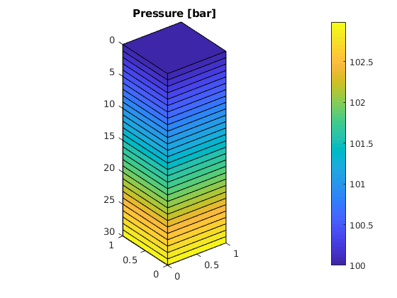
<html>
% <p><font size="-1
Single-phase Compressible AD Solver
Generated from flowSolverTutorialAD.m
The purpose of the example is to give the first introduction to how one can use the automatic differentiation (AD) class in MRST to write a flow simulator for a compressible single-phase model. For simplicity, the reservoir is assumed to be a rectangular box with homogeneous properties and no-flow boundaries. Starting from a hydrostatic initial state, the reservoir is produced from a horizontal well that will create a zone of pressure draw-down. As more fluids are produced, the average pressure in the reservoir drops, causing a gradual decay in the production rate. Suggested reading:
Set up model geometry
Rectangular 200-by-200-by-50 m^3 reservoir represented as a uniform 10-by-10-by-10 Cartesian grid. The grid is constructed using one of the standard grid-factory routines from MRST. Notice that we need to explicitly call the geometry processing routine computeGeometry to get cell and face centroids, cell volumes, and face areas needed for the finite-volume discretization of the flow equations.
[nx, ny, nz] = deal( 10,  10, 10);
[Dx, Dy, Dz] = deal(200, 200, 50);
G = cartGrid([nx, ny, nz], [Dx, Dy, Dz]);
G = computeGeometry(G);

plotGrid(G), view(3), axis tight
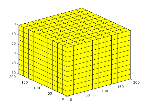
Define compressible rock model
For this problem we use a rock of constant compressibility. The pore-volume is therefore a simple analytic function of fluid pressure.
rock = makeRock(G, 30*milli*darcy, 0.3);

cr   = 1e-6/barsa;
p_r  = 200*barsa;
pv_r = poreVolume(G, rock);
pv   = @(p) pv_r .* exp(cr * (p - p_r));
p    = linspace(100*barsa, 220*barsa, 50);

plot(convertTo(p, barsa), pv_r(1) .* exp(cr * (p - p_r)), 'LineWidth', 2);
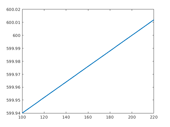
Define model for compressible fluid
the single-phase fluid is assumed to have constant compressibility. The fluid density is therefore a simple analytic function of pressure.
mu    = 5*centi*poise;
c     = 1e-3/barsa;
rho_r = 850*kilogram/meter^3;
rhoS  = 750*kilogram/meter^3;
rho   = @(p) rho_r .* exp(c * (p - p_r));

plot(convertTo(p, barsa), rho(p), 'LineWidth', 2)
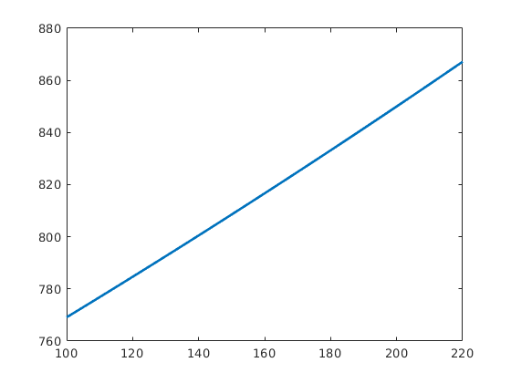
Assume a single horizontal well
The well is perforated in eight
nperf = 8;
I = repmat(2, [nperf, 1]);
J = (1 : nperf).' + 1;
K = repmat(5, [nperf, 1]);

cellInx = sub2ind(G.cartDims, I, J, K);
W = addWell([], G, rock, cellInx, 'Name', 'P1', 'Dir', 'y' );
Impose vertical equilibrium
We derive the initial pressure distribution by solving the intial value problem
To integrate this equation, we use the built-in ode23 solver. Notice also that the convention is MRST is that the z-direction points downward and hence the z-component of the gravity vector is positive.
gravity reset on, g = norm(gravity);
[z_0, z_max] = deal(0, max(G.cells.centroids(:,3)));
equil  = ode23(@(z,p) g .* rho(p), [z_0, z_max], p_r);
p_init = reshape(deval(equil, G.cells.centroids(:,3)), [], 1);  clear equil
Plot well and initial pressure
Since the well is inside the reservoir, we remove a section around the well so that we can see the well path
clf
show = true([G.cells.num, 1]);
cellInx = sub2ind(G.cartDims, ...
   [I-1; I-1; I; I;   I(1:2) - 1], ...
   [J  ; J;   J; J;   nperf  + [2 ; 2]], ...
   [K-1; K;   K; K-1; K(1:2) - [0 ; 1]]);

show(cellInx) = false;

plotCellData(G, convertTo(p_init, barsa), show, 'EdgeColor', 'k')
plotWell(G, W, 'height', 10)
view(-125, 20), camproj perspective
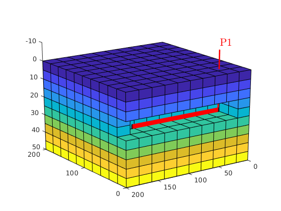
Compute transmissibilities on interior connections
We define the transmissibilities as the harmonic average of one-sided transmissibilities computed from cell properties (vector from cell centroid to face centroid, face areas, and cell permeabilities).
N  = double(G.faces.neighbors);
intInx = all(N ~= 0, 2);
N  = N(intInx, :);                            % Interior neighbors
hT = computeTrans(G, rock);                   % Half-transmissibilities
cf = G.cells.faces(:,1);                      % Map: cell -> face number
nf = G.faces.num;                             % Number of faces
T  = 1 ./ accumarray(cf, 1 ./ hT, [nf, 1]);   % Harmonic average
T  = T(intInx);                               % Restricted to interior
Define discrete operators
We use MATLAB®’s built-in sparse matrix type to form discrete gradient and divergence operators on the grid’s interior connections and active cells, respectively. The discrete gradient operator maps from cell pairs to faces and is defined as the difference in the cell values on opposite sides of the face. The discrete divergence operator is a linear mapping from faces to cells and can be computed as the adjoint of the discrete gradient operator. The divergence operator represent the sum of all outgoing fluxes from a cell. We furthermore create an operator that computes averages on the interior connections from cell values in the connecting cells. This operator is used to define fluid densities on the model’s connections.
n = size(N, 1);
C = sparse(repmat((1 : n).', [2, 1]), N, ...
           repmat([-1, 1], [n, 1]), n, G.cells.num);
grad = @(x) C * x;
div  = @(x)-C' * x;
avg  = @(x) 0.5 * (x(N(:,1)) + x(N(:,2)));
spy(C)
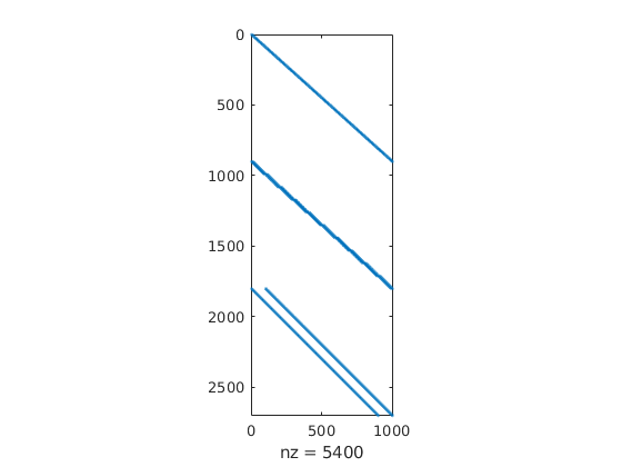
The discrete operators, together with the transmissibility T and the vector pv of pore volumes, represent all the information we need from the geological model to discretize the flow equations using a first-order finite-volume method. In principle, we could therefore have deleted the G and rock objects. However, the common practice in MRST is to keep these objects throughout the simulation. The grid will, for instance, be needed for plotting purposes.
Define flow equations
The flow equations are discretized in time by the backward Euler method and in space using a finite-volume method. To solve the equations, we will write the equations on residual form, F(x) = 0, and use a standard Newton-Raphson method to solve the resulting system of nonlinear equations. To define F(x), we introduce a number of anonymous functions that each define one part of the flow equations. We start by defining the anonymous functions for Darcy’s law (called flux) and for the continuity equation (called presEq).
gradz  = grad(G.cells.centroids(:,3));
flux   = @(p)  -(T / mu).*(grad(p) - g*avg(rho(p)).*gradz);
presEq = @(p,p0,dt) (1 / dt) * (pv(p).*rho(p) - pv(p0).*rho(p0)) ...
                      + div(avg(rho(p)) .* flux(p));
Define well equations
The well is describe by four equations:
wc = W(1).cells; % connection grid cells
WI = W(1).WI;    % well-indices
dz = W(1).dZ;    % connection depth relative to bottom-hole

p_conn  = @(bhp)  bhp + g*dz.*rho(bhp); %connection pressures
q_conn  = @(p,bhp) WI .* (rho(p(wc)) / mu) .* (p_conn(bhp) - p(wc));

rateEq = @(p,bhp,qS)  qS - sum(q_conn(p, bhp))/rhoS;
ctrlEq = @(bhp)       bhp - 100*barsa;
Initialize for solution loop
By nesting and evaluating all the anonymous functions defined above in all cells of the reservoir, we can evaluate the residual F(x). The well equations are accounted for by evaluating the equations that depend on reservoir pressure are evaluated in all cells containing a well perforation. However, to solve the problem F(x)=0 and find the unknown x, we need to compute the gradient dF/dx. To this end, we will use automatic differentiation (AD), which is a technique for numerical evaluating the derivatives of a function specified by a computer program. Using this technique, all we have to do is implement the equations (as we did above), declar the input variables as automatic differentiation variables, and when our any are evaluated, we get both the residual value and the derivatives with respect the the AD variables.
% Initialize primary unknowns as AD variables and keep track of their
% respective indices in the overall vector of unknowns
[p_ad, bhp_ad, qS_ad] = initVariablesADI(p_init, p_init(wc(1)), 0);
nc = G.cells.num;
[pIx, bhpIx, qSIx] = deal(1:nc, nc+1, nc+2);

% Parameters specifying the simulation
numSteps = 52;                  % number of time-steps
totTime  = 365*day;             % total simulation time
dt       = totTime / numSteps;  % constant time step
tol      = 1e-5;                % Newton tolerance
maxits   = 10;                  % max number of Newton its

% Empty structure for keeping the solution
sol = repmat(struct('time', [], 'pressure', [], 'bhp', [], 'qS', []), ...
             [numSteps + 1, 1]);

% Initial state
sol(1)  = struct('time', 0, 'pressure', value(p_ad), ...
                 'bhp', value(bhp_ad), 'qS', value(qS_ad));
Main loop
t = 0; step = 0;
while t < totTime,
   t = t + dt;
   step = step + 1;
   fprintf('\nTime step %d: Time %.2f -> %.2f days\n', ...
           step, convertTo(t - dt, day), convertTo(t, day));

   % Newton loop
   converged = false;
   p0  = value(p_ad); % Previous step pressure
   nit = 0;
   while ~converged && (nit < maxits),
      % Add source terms to homogeneous pressure equation:
      eq1     = presEq(p_ad, p0, dt);
      eq1(wc) = eq1(wc) - q_conn(p_ad, bhp_ad);

      % Collect all equations
      eqs = {eq1, rateEq(p_ad, bhp_ad, qS_ad), ctrlEq(bhp_ad)};

      % Concatenate equations and solve for update. Concatenating the
      % equations will assemble the Jacobians associated with each
      % subequation into a block-structured Jacobian matrix for the full
      % system
      eq  = cat(eqs{:});
      J   = eq.jac{1};  % Jacobian
      res = eq.val;     % residual
      upd = -(J \ res); % Newton update

      % Update variables
      p_ad.val   = p_ad.val   + upd(pIx);
      bhp_ad.val = bhp_ad.val + upd(bhpIx);
      qS_ad.val  = qS_ad.val  + upd(qSIx);

      residual  = norm(res);
      converged = ~(residual > tol);
      nit       = nit + 1;
      fprintf('  Iteration %3d:  Res = %.4e\n', nit, residual);
   end

   if ~ converged,
      error('Newton solves did not converge')
   else % store solution
      sol(step+1)  = struct('time', t, 'pressure', value(p_ad), ...
                            'bhp', value(bhp_ad), 'qS', value(qS_ad));
   end
end
Time step 1: Time 0.00 -> 7.02 days
  Iteration   1:  Res = 1.0188e+07
  Iteration   2:  Res = 3.1032e-02
  Iteration   3:  Res = 1.8547e-05
  Iteration   4:  Res = 5.4513e-12

Time step 2: Time 7.02 -> 14.04 days
...
Plot production rate and pressure decay
clf
[ha, hr, hp] = plotyy(...
   convertTo([sol(2:end).time], day), ...
   convertTo(-[sol(2:end).qS], meter^3/day), ...
   ...
   convertTo([sol(2:end).time], day), ...
   convertTo(mean([sol(2:end).pressure], 1), barsa), 'stairs', 'plot');

set(ha, 'FontSize', 16);
set(hr, 'LineWidth', 2);
set(hp, 'LineStyle', 'none', 'Marker', 'o', 'LineWidth', 1);
set(ha(2), 'YLim', [100, 210], 'YTick', 100:50:200);

xlabel('time [days]');
ylabel(ha(1), 'rate [m^3/day]');
ylabel(ha(2), 'avg pressure [bar]');
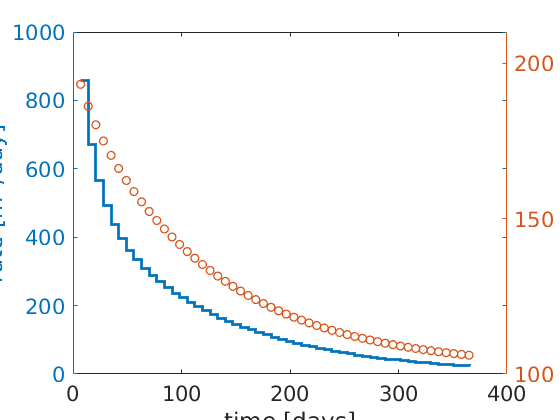
Plot pressure evolution
clf
steps = [2, 5, 10, 20];
for i = 1 : numel(steps),
   subplot(2,2,i)
   plotCellData(G, convertTo(sol(steps(i)).pressure, barsa), ...
                show, 'EdgeColor', repmat(0.5, [1, 3]))

   plotWell(G, W)

   view(-125, 20), camproj perspective

   caxis([115, 205])
   axis tight off;

   text(200, 170, -8, ...
        sprintf('%.1f days', convertTo(steps(i)*dt, day)), 'FontSize', 14)
end

h = colorbar('South', 'Position', [0.1, 0.05, 0.8, .025]);
colormap(jet(55));
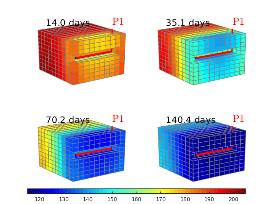
Copyright Notice
Introduction to Automatic Differentiation
Generated from tutorialAD.m
Automatic differentiation is, quoting from Wikipedia: “_a set of techniques to numerically evaluate the derivative of a function specified by a computer program. AD exploits the fact that every computer program, no matter how complicated, executes a sequence of elementary arithmetic operations (addition, subtraction, multiplication, division, etc.) and elementary functions (exp, log, sin, cos, etc.). By applying the chain rule repeatedly to these operations, derivatives of arbitrary order can be computed automatically, accurately to working precision, and using at most a small constant factor more arithmetic operations than the original program._” In MRST, we have implemented automatic differentiation using operator overloading. In this tutorial, we give you a very brief introduction to our implementation of AD, which is specifically geared towards discretization of partial differential equations and computation with long vectors and sparse matrices. Unlike many other implementations of AD, we have chosen to keep individual Jacobians as a list of sparse matrices and not automatically expand into a large global matrix. This ensures efficiency and flexibility in manipulating matrix blocks corresponding to subequations of (complex) equation systems. Suggested reading:
Simple formula using two scalars
Compute z = 3 exp(-xy) and its partial derivatives wrt x and y. First, we compute it manually and then using automatic differentiation (AD). To understand what is going on behind the curtains when using AD, you can set a breakpoint at line 13 and use the ‘Step into’ function to step through the different functions that are invoked when evaluating z
[x,y]=deal(1,2);
disp('Manually computed:')
disp([1 -y -x]*3*exp(-x*y))

disp('Automatic differentiation:')
[x,y] = initVariablesADI(1,2);
z = 3*exp(-x.*y)                                                           %#ok<*NOPTS>
Manually computed:
    0.4060   -0.8120   -0.4060

Automatic differentiation:

z =

  ADI with properties:
...
Demonstrate the importance of vectorization
m = 14;
[n,t1,t2,t3,t4] = deal(zeros(m,1));
clc
disp('Table: timing for differentiation of z=xy');
disp('   nvec  analytic     vectorized   loop+mtimes  loop+times');
disp('   --------------------------------------------------------');
for i = 1:m
   n(i) = 2^(i-1);
   xv = rand(n(i),1); yv=rand(n(i),1);
   [x,y] = initVariablesADI(xv,yv);
   tic, z = xv.*yv; zx=yv; zy = xv; t1(i)=toc;                             %#ok<*NASGU>
   tic, z = x.*y;                   t2(i)=toc;
   if i<17
      tic, for k =1:n(i), z(k)=x(k)*y(k); end;  t3(i)=toc;
      tic, for k =1:n(i), z(k)=x(k).*y(k); end; t4(i)=toc;
   end
   fprintf('%7d: %6.5f sec, %6.5f sec, %6.5f sec, %6.5f sec\n', ...
      n(i), t1(i), t2(i), t3(i), t4(i))
end
disp('   --------------------------------------------------------');
disp('');
loglog(n,t1,'-*',n,t2,'-+',n,t3,'-o',n,t4,'-s');
legend('analytical','vectorized','for+mtimes','for+times','Location','NorthEast');
Table: timing for differentiation of z=xy
   nvec  analytic     vectorized   loop+mtimes  loop+times
   --------------------------------------------------------
      1: 0.00015 sec, 0.00023 sec, 0.00635 sec, 0.00045 sec
      2: 0.00039 sec, 0.00051 sec, 0.00587 sec, 0.00125 sec
      4: 0.00007 sec, 0.00013 sec, 0.00402 sec, 0.00162 sec
      8: 0.00004 sec, 0.00012 sec, 0.00170 sec, 0.00185 sec
     16: 0.00048 sec, 0.00037 sec, 0.00358 sec, 0.00487 sec
...
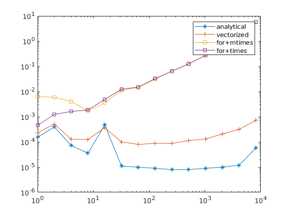
Use automatic differentation to assmble a linear system
x = initVariablesADI(zeros(3,1));
eq1 = [ 3,  2, -4]*x + 5;
eq2 = [ 1, -4,  2]*x + 1;
eq3 = [-2,- 2.  4]*x - 6;
eq = cat(eq1,eq2,eq3);
disp(eq.jac{1})
disp(eq.val)
u  = -eq.jac{1}\eq.val; disp(u)
3     2    -4
     1    -4     2
    -2    -2     4

     5
     1
    -6

...
Use AD to solve the nonlinear Rosenbrock problem
Problem: minimize f(x,y) = (a-x)^2 + b(y-x^2)^2 = 0 The solution is (a,a^2). A necessary condition for minimum is that grad(f(x,y))=0, which gives two residual equations 2(a-x) - 4bx(y-x^2) = 0 2b(y-x^2) = 0 Here, we set a=1 and b=100
[a,b,tol] = deal(1,100,1e-6);
[x0,incr] = deal([-.5;4]);
while norm(incr)>tol
    x = initVariablesADI(x0);
    eq = cat( 2*(a-x(1)) - 4*b.*x(1).*(x(2)-x(1).^2), ...
        2*b.*(x(2)-x(1).^2));
    incr = - eq.jac{1}\eq.val;
    x0 = x0 + incr;
end
Slightly more elaborate version with plotting
a,b] = deal(1,100);
fx = @(x) 2*(a-x(1)) - 4*b.*x(1).*(x(2)-x(1).^2);
fy = @(x) 2*b.*(x(2)-x(1).^2);
[tol,res,nit] = deal(1e-6, inf,0);
x = [-.5 4];
while res>tol && nit<100
    nit = nit+1;
    xd = initVariablesADI(x(end,:)');
    eq = cat(fx(xd),fy(xd));
    incr = - eq.jac{1}\eq.val;
    res = norm(incr);
    x = [x; x(end,:)+incr']; %#ok<AGROW>
end

% Plot solution: use modified colormap to clearly distinguish the region
% with lowest colors. Likewise, show the value of f per iteration on a
% nonlinear scale, i.e., f(x,y)^0.1
subplot(4,1,1:3);
f = @(x,y) (a-x).^2 + b.*(y-x.^2).^2;
[xg, yg] = meshgrid(-2:0.2:2, -1.5:0.2:4);
surf(xg,yg,reshape(f(xg(:), yg(:)),size(xg))); shading interp
hold on;
plot3(x(:,1),x(:,2),f(x(:,1),x(:,2)),'-or', 'LineWidth', 2, ...
    'MarkerSize',8,'MarkerEdgeColor','k','MarkerFaceColor','r');
hold off
view(-130,45); axis tight; colormap([.3 .3 1; jet(99)]);
subplot(4,1,4)
bar(f(x(:,1),x(:,2)).^.1,'b'); axis tight; set(gca,'YTick',[]);
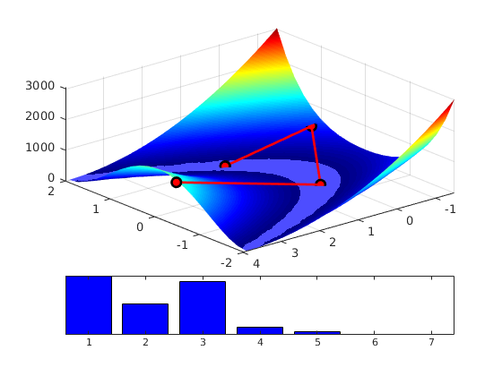
Basic Objects in MRST Workflows
Generated from tutorialBasicObjects.m
The most fundamental object in MRST is the grid. This dual purpose object both discretises a model’s geometry and serves as a database to which static and dynamic properties and other objects are attached. Examples of such associate data are
This example explores a number of ways of constructing grids with degrees of complexity varying from simple Cartesian models with synthetic values for the porosity and permeability through to fully unstructured models in the industry-standard corner-point format. We moreover introduce a collection of open datasets that are either hosted on the MRST website or published on other sites.
Activate Requisite Modules
- MRST comes equipped with a graphical user interface for interactively exploring static and dynamic properties attached to a grid. We enable this functionality by activating the
mrst-guimodule that is provided in the MRST distribution. Function is the gateway to MRST’s module system. Modules are add-on features that can be enabled and disabled on demand. For now we will not discuss this feature any further, but interested readers can find out more about it in the Release Notes for MRST 2014a. We also activate the
deckformatmodule, which contains functionality for reading and parsing data files given in the industry-standard ECLIPSE format.
mrstModule add mrst-gui deckformat ad-core
Simple Cartesian Model
We start with a simple Cartesian model. Function cartGrid creates shoe-box like models using a pair (for 2D) or triplet (for 3D) of integers representing the number of cells in each cardinal direction. Unless otherwise instructed, cartGrid will create cells of unit dimension (one metre in each direction). Consequently, the total size of the model geometry depends on the number of cells. This behaviour may be altered by passing the total size of the shoe-box as a second argument. The first grid is a 5-by-5-by-10 discretisation of the unit cube. We can visualise the resulting geometry using function plotGrid.
G = cartGrid([5, 5, 10], [1, 1, 1].*meter);

plotGrid(G), view([-40, 32]), xlabel('x'), ylabel('y'), zlabel('Depth')
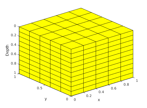
Populate Model
Function makeRock creates a structure that holds the porosity and permeability fields, customarily referred to as rock throughout the MRST package. Function plotCellData can then be employed to visualise the porosity field.
rock = makeRock(G, 100*milli*darcy, 0.3);
plotCellData(G, rock.poro)
view([-40, 32]), xlabel('x'), ylabel('y'), zlabel('Depth'), colorbar
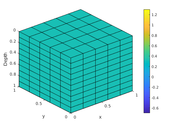
Deactivate Selected Cells
Function gridLogicalIndices will, provided the grid has an underlying Cartesian structure, compute (I,J,K) triplets either for all grid cells or a user-selected subset of those grid cells. We can, for instance, use these values to pick out a subset of the cells and exclude those cells from the model using function removeCells.
We’ll pick out the 3-by-3-by-6 sub-cube in the centre of the model. This cube can be identified by the (I,J) indices having values in the range 2:4 and the K indices being in the range 3:8. Combining this with logical expressions means we can extract the subset in an economical way using MATLAB®’s built-in function all.
pick_ij = false([ 5, 1]); pick_ij(2 : 4) = true;
pick_k = false([10, 1]); pick_k (3 : 8) = true;
ijk = gridLogicalIndices(G);
c = all([pick_ij([ijk{[1, 2]}]), pick_k(ijk{3})], 2);
Gr = removeCells(G, c);
clf
plot_cells = true([5, 1]); plot_cells([1, 2]) = false;
plotGrid(G, 'FaceColor', 'none', 'EdgeAlpha', 0.6, ...
'EdgeColor', [0.6, 0.4, 0.5], 'LineWidth', 1.2)
plotGrid(Gr, plot_cells(ijk{2}(~c)))
view([-48, 25]), xlabel('x'), ylabel('y'), zlabel('Depth')
material shiny, camlight(-60, -50)
for k = 1:3, camlight(-60, 50), end
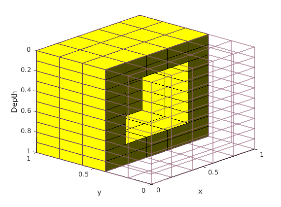
Geostatistical Distribution of Petrophysical Properties
MRST does not have advanced geostatistical functionality. The two functions logNormLayers and gaussianField may be used to sample random fields in a spatial region with various degrees of correlation, but we recommend that more complete geostatistical software be employed in a more realistic situations. Here, we simply demonstrate that we can visualise spatially varying data. Note that the formula that derives the permeability field from the porosity fields makes certain simplifying assumptions about the nature of the rock and its grains. Function compressRock from the deckformat module is useful when extracting the petrophysical properties that pertain to a model’s active cells only.
poro = reshape(gaussianField(G.cartDims, [0.2, 0.4]), [], 1);
perm = poro.^3 .* (1e-5)^2 ./ (0.81 * 72 * (1 - poro).^2);
rock = makeRock(G, perm, poro);
rock_r = compressRock(rock, Gr.cells.indexMap);
clf, subplot(1,2,1)
plotCellData(G, log10(convertTo(rock.perm, milli*darcy)))
view([-48, 20]), xlabel('x'), ylabel('y'), zlabel('Depth')
subplot(1,2,2)
plotGrid(G, 'FaceColor', 'none', 'EdgeAlpha', 0.4, ...
'EdgeColor', [0.6, 0.4, 0.5], 'LineWidth', 1.2)
plotCellData(Gr, log10(convertTo(rock_r.perm, milli*darcy)), ...
plot_cells(ijk{2}(~c)))
view([-48, 20]), xlabel('x'), ylabel('y'), zlabel('Depth')
material shiny, camlight(-60, -50)
for k = 1:3, camlight(-60, 50), end
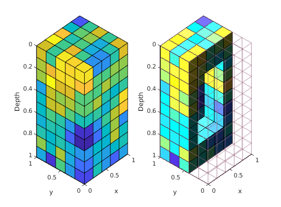
Unstructured Grids in Corner-Point Format
MRST provides mature support for unstructured grids in the corner-point format as represented in the ECLIPSE reservoir simulator. There are multiple example grids in the testgrids directory. Here, however, we will use one of the datasets known to MRST. Function getAvailableDatasets contains the list of known datasets. The second return value, present, is a logical array that states whether or not the corresponding dataset is available on the local computer system.
[info, present] = getAvailableDatasets;
display([ { info(present).name } ; ...
{ info(present).modelType } ] .')
0×0 empty cell array
Construct grid and properties from ECLIPSE-type input.
Function processGRDECL constructs MRST grids from ECLIPSE-style input. Such data can be input using either function readGRDECL or function readEclipseDeck. The latter is intended for complete simulation cases, i.e., ECLIPSE-style .DATA files, whereas the former reads loosely coupled grid data and does not form a state machine to handle temporally changing wells and related constraints.
MRST’s function getDatasetPath returns the full path of a particular dataset on the local computer system. We take care to convert the input data to MRST’s strict SI only unit conventions in the process. Using strict SI units means that no solver or simulator needs to be aware of any particular unit convention. Note moreover that in order to visualise the pore-volume field we need to compute the bulk (geometric) volume of all grid cells. This calculation, along with cell and connection centroids, connection areas, and connection normals, is affected by MRST’s built-in function computeGeometry.
grdecl = readGRDECL(fullfile(getDatasetPath('BedModel2'), ...
'BedModel2.grdecl'));
grdecl = convertInputUnits(grdecl, getUnitSystem('LAB'));
G = computeGeometry(processGRDECL(grdecl));
rock = compressRock(grdecl2Rock(grdecl), G.cells.indexMap);
pvol = poreVolume(G, rock);
clf
plotCellData(G, convertTo(pvol, (centi*meter)^3), 'EdgeAlpha', 0.1), colorbar
view([-32, 22]), xlabel('x'), ylabel('y'), zlabel('Depth'), grid on
Error using input
Cannot call INPUT from EVALC.
Error in downloadDataset>confirm_download (line 184)
response = input(prompt, 's');
Error in downloadDataset>do_download (line 163)
do_get = confirm_download(info);
...
This model is a high-resolution discretisation of a 30-by-30-by-6 cm^3 sedimentary bed that contains six different rock types. The model is represented by a grid with 30-by-30-by-333 cells of which nearly 70% are inactive due to pinch-out. Moreover, most of the remaining active cells have degenerate geometry. For visualisation purposes we add the rock types–represented as integer values in the SATNUM array of the input data–to the rock structure and then launch the plotToolbar viewer to let you interactively inspect the model in more detail. The ‘ijk’ button allows you to view the model in logical space rather than in physical space which is useful to reveal the structure of the model. Using the histogram picker we can further inspect the distribution of each individual rock type throughout the model. We also recommend using the interactive slice plane to view the interior of the model. This part is normally obstructed when statically visualising the geometry by means of the lower-level tool plotCellData.
rock.rocktype = grdecl.SATNUM(G.cells.indexMap);
plotToolbar(G, rock,'field','rocktype');
view([-32, 22]), xlabel('x'), ylabel('y'), zlabel('Depth'), axis tight
Initialise Complete Simulation Case From ECLIPSE Data
MRST is able to use complete ECLIPSE simulation cases as input and construct objects that are usable in an MRST simulation scenario. This functionality is available in the deckformat module and centred around the functions readEclipseDeck, convertDeckUnits, initEclipseGrid, and processWells. The initEclipseProblemAD function available in the ad-core module calls those helper functions and others to create a fully formed simulation model object, initial distributions of pressures and masses and a set of dynamic well controls, boundary conditions and source terms known as the simulation schedule. We furthermore remark that the simulation grid is stored as the data field G of the model object. Here we visualise the initial phase distribution in the well-known Ninth SPE Comparative Solution Project, plotting the oil phase as green, the gas phase as red and the water phase as blue.
input = fullfile(getDatasetPath('SPE9'), 'BENCH_SPE9.DATA');
deck = convertDeckUnits(readEclipseDeck(input));
[state0, model, schedule] = initEclipseProblemAD(deck);
name_wells = @(prefix, n) ...
arrayfun(@(i) sprintf('$\\mathit{%s}_{%02d}$', prefix, i), ...
1 : n, 'UniformOutput', false);
wells = schedule.control(1).W;
is_inj = [ wells.sign ] > 0;
wname = name_wells('I', sum(is_inj));
[wells(is_inj).name] = wname{:};
is_prod = [ wells.sign ] < 0;
wname = name_wells('P', sum(is_prod));
[wells(is_prod).name] = wname{:};
clf
plotCellData(model.G, state0.s(:, [3, 2, 1])), axis tight, grid on
[htop, htext, hs, hline] = plotWell(model.G, wells);
view([55, 40]), xlabel('x'), ylabel('y'), zlabel('Depth')
Once initialised, this model can now be simulated using the set of dynamic well constraints. As an example of such a simulation, one that uses MRST’s automatic (algorithmic) differentiation framework, we suggest the reader review our SPE-9 black-oil simulation tutorial. To get a list of other tutorials of the same kind, type mrstExamples ad-core ad-blackoil.
Copyright Notice
Visualizing in MRST
Generated from tutorialPlotting.m
MRST contains a suite of visualization routines which make it easy to create visualizations of grids and results. This tutorial show how to visualize grids, subsets of grids and details the different routines included in MRST.
PLotting grids
The plotGrid function is an essential part of MRST’s visualization routines. It simply draws a grid to a figure with a reversed z axis.
G = cartGrid([10, 10, 3]);
G = computeGeometry(G);
clf;
plotGrid(G)
view(30,50)
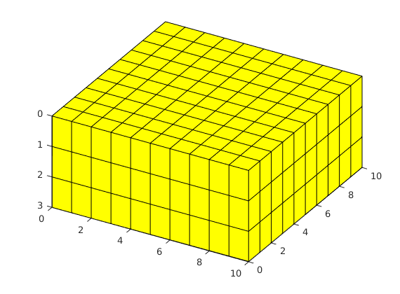
MRST and patch
All grid plotting routines are based on MATLAB’s patch routine, which enables plotting of general polygons. Any keyword arguments will be passed on to patch, which makes it possible to alter many attributes. For instance, we can replot the grid with partially transparent edges and faces in another color:
clf;
plotGrid(G, 'EdgeAlpha', 0.1, 'FaceColor', 'blue')
view(30,50)
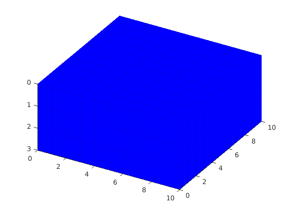
plotGrid and subsets
plotGrid’s second argument corresponds to a list of cells to be plotted. This can be either logical indices (a logical vector of length G.cells.num will plot Cell i if the ith element of the vector is true) or an explicit list of indices, i.e. the cell numbers to be plotted. To demonstrate this, we will plot all indices with equal values in a different color. Note that the plotting routines do not reset the figure between plots, making it easy to create compositions of different plots.
clf;
equal_index = mod(1:G.cells.num,2) == 0;
plotGrid(G, equal_index, 'FaceColor', 'red')
plotGrid(G, ~equal_index, 'FaceColor', 'blue')
view(30,50)
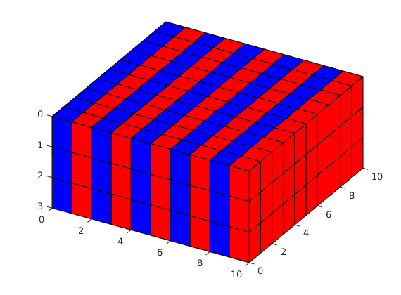
Plotting cell properties
To illustrate the visualization of cell properties, we will use routines from the incomp module to set up and solve a simple flow problem. This is only meant as an example for the visualization and will not be covered thourougly.
mrstModule add incomp
gravity off % Disable gravity
rock = makeRock(G, 100*milli*darcy, 0.5); % Uniform rock properties
fluid = initSimpleFluid( ...
% A simple fluid
'mu' , [ 1, 10]*centi*poise , ...
% - viscosity
'rho', [1014, 859]*kilogram/meter^3, ...
% - density
'n' , [ 2, 2]); % - quadratic Corey relperms
W = verticalWell([], G, rock, 1, 1, [], ...
% Injector in cell (1,1)
'Type', 'bhp' , 'Val', 1*barsa(), ...
% - bhp=1 bar
'Radius', 0.1, 'InnerProduct', 'ip_tpf', ...
'Comp_i', [0, 1]);
W = verticalWell(W, G, rock, 10, 10, [], ...
% Producer in cell (10,10)
'Type', 'bhp' , 'Val', 0*barsa(), ...
% - bhp=0 bar
'Radius', 0.1, 'InnerProduct', 'ip_tpf', ...
'Comp_i', [1, 0]);
sol = initState(G, [], 0, [1, 0]); % Initial: filled with phase 1
% Compute transmissibility and define function handles for solvers to avoid
% having to retype parameters that stay constant throught the simulation
T = computeTrans(G, rock);
psolve = @(state) incompTPFA(state, G, T, fluid, 'wells', W);
tsolve = @(state, dT) implicitTransport(state, G, dT, rock, fluid, 'wells', W);
Plot the pressure distribution
Generally seeing only the grid is not that interesting. If we want to show actual values, we need to use plotCellData. Let us solve the reservoir pressure and plot it:
sol= psolve(sol);
clf;
plotCellData(G, sol.pressure)
colorbar, view(30,50)
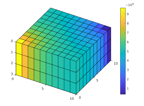
Plot subset of data
We can observe that the pressure has its largest values in the wells, which makes it seem that the pressure is almost homogeneous inside the domain. Let us then plot pressure values for the middle of the domain. We also plot an empty grid to see where we are actually plotting. In addition, we use the plotWell function to show wells.
[i,j,k] = ind2sub(G.cartDims, 1:G.cells.num);
clf;
plotGrid(G, 'FaceAlpha', 0, 'EdgeAlpha', .1)
plotCellData(G, sol.pressure, j == round(G.cartDims(2)/2))
plotWell(G, W); view(30,50)
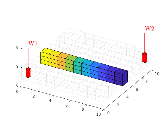
plotFaces - plotting face values
Some data is given at a per face basis instead of cells. For this purpose we have plotFaces and plotFaceData which are analogous to plotGrid and plotCellData respectively. To illustrate this function, we plot all faces having positive normal in the z-direction
clf;
plotFaces(G, find(G.faces.normals(:,3)>0));
view(30,50);
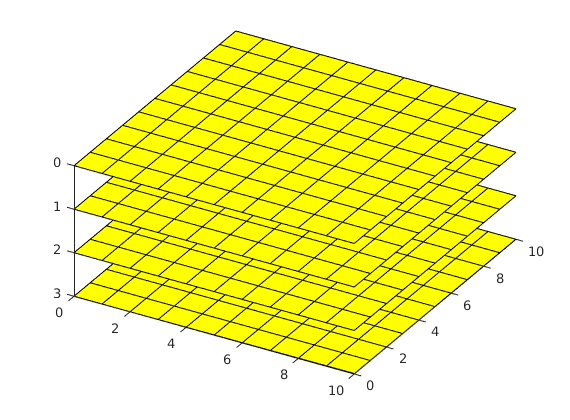
plotFaceData
plotFaceData lets us plot face values, for instance when dealing with fluxes and faults. For an example, let us plot the faces colored by the z values of the face centroids.
clf;
plotFaceData(G, G.faces.centroids(:,3));
view(30,50);
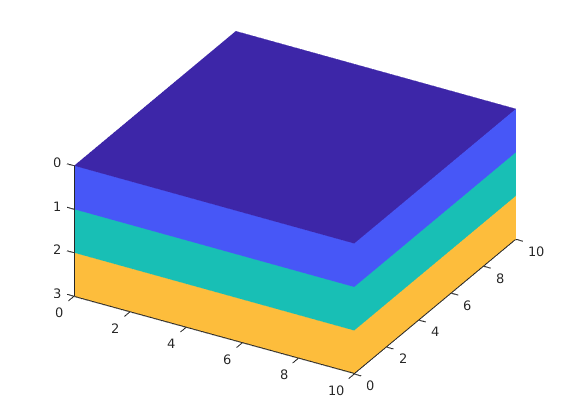
Animated example
We will now simulate a simple transport problem between the wells and create an animation that shows how the solution develops over time. To this end, we plot the empty grid and the wells, and in each time step only show the saturation in the cells where the saturation of the injected phase is above a threshold, here 0.05. Here, we solve and plot the solution simulaneously. We also store the time steps in a cell array so that they can be extracted after the simulation has finished
% Set up static parts of the plot
clf
plotGrid(G, 'FaceAlpha', 0, 'EdgeAlpha', .1)
plotWell(G, W);
view(30,50); pause(1)
hs = []; % handle for saturation plot, empty initially
% Perform simulation
dT = 10*day;
solutions = cell(20,1);
for i = 1:20
sol = tsolve(sol, dT);
sol = psolve(sol);
solutions{i} = sol;
delete(hs)
hs = plotCellData(G, sol.s(:,2), sol.s(:,2)>0.05);
drawnow, pause(.5)
end
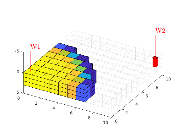
Alternatively, use plotGridVolumes for the same purpose
The function plotGridVolumes is an alternative to plotCellData. While more computationally intensive, it plots interpolated surfaces corresponding to specific values of the saturation, giving a better indication of the saturation front and a less clear indication of the saturation mixture in sationary areas. These functions can be combined depending on the nature of the data set.
for i = 1:20
clf;
sol = solutions{i};
plotGridVolumes(G, sol.s(:,2), 'basealpha', 2)
plotGrid(G, 'FaceAlpha', 0, 'EdgeAlpha', .1);
plotWell(G, W);
view(30,50);
pause(.5)
end
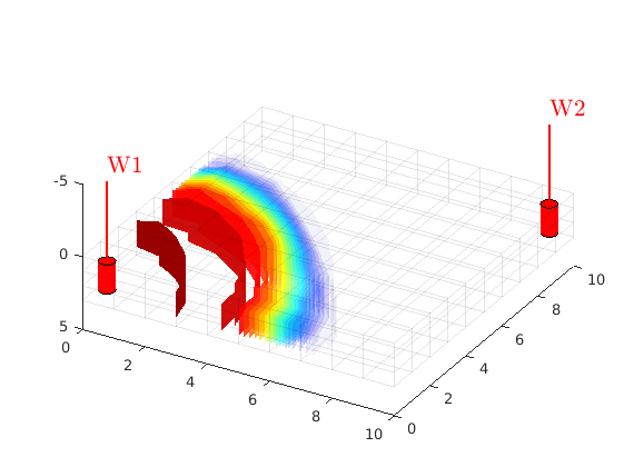
<html>
% <p><font size="-1
Stair-stepped grid
Generated from showCaseB4.m
clf
pltarg = {'FaceColor', [1 1 .5], 'EdgeAlpha',.1};
grdecl = readGRDECL(fullfile(getDatasetPath('CaseB4'),'stairstep_36x48.grdecl'));
Gs = processGRDECL(grdecl);
Gs = computeGeometry(Gs);
plotGrid(Gs,pltarg{:});
set(gca,'dataa',[15 20 1])
axis tight off, view(150,30), zoom(1.2)
set(gca,'Clipping','off')
Error using input
Cannot call INPUT from EVALC.
Error in downloadDataset>confirm_download (line 184)
response = input(prompt, 's');
Error in downloadDataset>do_download (line 163)
do_get = confirm_download(info);
...
cut_grdecl = cutGrdecl(grdecl, [12 20; 13 23; 1 12]);
g = processGRDECL(cut_grdecl);
clf
plotGrid(g, pltarg{:}),
axis tight off, view(150,50), zoom(1.2)
set(gca,'Clipping','off')
Corner-point grid
clf
grdecl = readGRDECL(fullfile(getDatasetPath('CaseB4'),'pillar_36x48.grdecl'));
Gp = processGRDECL(grdecl);
Gp = computeGeometry(Gp);
plotGrid(Gp, pltarg{:});
set(gca,'dataa',[15 20 1])
axis tight off, view(150,30), zoom(1.2)
set(gca,'Clipping','off')
cut_grdecl = cutGrdecl(grdecl, [12 20; 13 23; 1 12]);
g = processGRDECL(cut_grdecl);
clf
plotGrid(g, pltarg{:}),
axis tight off, view(150,50), zoom(1.2)
set(gca,'Clipping','off')
Visualize results
lf
set(gcf,'Position', [300 450 1000 330]);
subplot(1,2,1);
plotGrid(Gs, pltarg{:});
set(gca,'dataaspect',[32 44 2.5])
axis tight off, view(104,28);
%
subplot(1,2,2);
plotGrid(Gp, pltarg{:});
set(gca,'dataaspect',[32 44 2.5])
axis tight off, view(104,28);
Visualizing the Johansen Data Set
Generated from showJohansen.m
The Johansen formation is a candidate site for large-scale CO2 storage offshore the south-west coast of Norway. The MatMoRA project has developed a set of geological models based on available seismic and well data. Herein, we will inspect one instance of the model in more detail.
Faults and active/inactive cells
We start by reading the model from a file in the Eclipse format (GRDECL), picking the sector model with five vertical layers in the Johansen formation and with five shale layers above and one below. The file contains both active and inactive cells. We take the chance that the inactive cells do not contain garbage and visualize the whole model, marking with red color all faults found during processing.
dpath = getDatasetPath('johansen');
sector = fullfile(dpath, 'NPD5');
filename = [sector, '.grdecl'];
grdecl = readGRDECL(filename); clear filename
actnum = grdecl.ACTNUM;
grdecl.ACTNUM = ones(prod(grdecl.cartDims),1);
G = processGRDECL(grdecl, 'checkgrid', false);
Error using input
Cannot call INPUT from EVALC.
Error in downloadDataset>confirm_download (line 184)
response = input(prompt, 's');
Error in downloadDataset>do_download (line 163)
do_get = confirm_download(info);
...
Plot the results
clf, subplot('position',[0.025 0.025 0.95 0.95]);
h = plotGrid(G,'FaceColor',.85*[1 1 1], 'FaceAlpha',.4,'EdgeColor','none');
plotFaces(G,find(G.faces.tag>0),'FaceColor','r','EdgeColor','none');
axis tight off; view(-145,60);
set(gca,'ZDir','normal'), camlight headlight, set(gca,'Zdir','reverse');
Next we mark the active part of the model
delete(h);
plotGrid(G,find(~actnum(G.cells.indexMap)), ...
'FaceColor',.85*[1 1 1], 'FaceAlpha',.4,'EdgeColor','none');
plotGrid(G,find(actnum(G.cells.indexMap)), ...
'FaceColor', 'b', 'FaceAlpha', 0.4,'EdgeColor','none');
view(15,40);
%set(gca,'ZDir','normal'), camlight headlight, set(gca,'Zdir','reverse');
Height map
It is only meaningful to show a height map of the active cells. Therefore, to inspect only the active model, we reset the ACTNUM field to its original values and recreate the grid. Now, inactive cells will be ignored and we therefore get a different unstructured grid.
grdecl.ACTNUM = actnum; clear actnum;
G = processGRDECL(grdecl); clear grdecl;
G = computeGeometry(G);
% Plotting a height map of the field using the z-component of the centroids
% of the cells
clf,
plotCellData(G,G.cells.centroids(:,3),'EdgeColor','k','EdgeAlpha',0.1);
colorbar, view(3), axis tight off, view(-20,40), zoom(1.2)
set(gca,'Clipping','off')
Porosity
The porosity data are given with one value for each cell in the model. We read all values and then pick only the values corresponding to active cells in the model.
clf
p = reshape(load([sector, '_Porosity.txt'])', prod(G.cartDims), []);
poro = p(G.cells.indexMap); clear p
plotCellData(G, poro,'EdgeColor','k','EdgeAlpha',0.1);
colorbarHist(poro,[0.09 0.31],'West',50); view(-45,15), axis tight off, zoom(1.2)
set(gca,'Clipping','off')
From the plot, it seems like the formation has been pinched out and only contains the shale layers in the front part of the model. We verify this by plotting a filtered porosity field in which all values smaller than or equal 0.1 have been taken out.
clf
view(-15,40)
plotGrid(G,'FaceColor','none','EdgeAlpha',0.1);
plotCellData(G, poro, poro>0.1, 'EdgeColor','k','EdgeAlpha',0.1);
colorbarHist(poro(poro>.1),[0.09 0.31],'West',50);
axis tight off, zoom(1.45), camdolly(0,.2,0);
set(gca,'Clipping','off')
Permeability
The permeability is given as a scalar field (Kx) similarly as the porosity. The tensor is given as K = diag(Kx, Kx, 0.1Kx) and we therefore only plot the x-component, Kx, using a logarithmic color scale.
clf
K = reshape(load([sector, '_Permeability.txt']')', prod(G.cartDims), []);
perm = bsxfun(@times, [1 1 0.1], K(G.cells.indexMap)).*milli*darcy; clear K;
rock = makeRock(G, perm, poro);
p = log10(rock.perm(:,1));
plotCellData(G,p,'EdgeColor','k','EdgeAlpha',0.1);
view(-45,15), axis tight off, zoom(1.2)
set(gca,'Clipping','off')
% Manipulate the colorbar to get the ticks we want
cs = [0.01 0.1 1 10 100 1000];
caxis(log10([min(cs) max(cs)]*milli*darcy));
h = colorbarHist(p,caxis,'West',100);
set(h, 'XTick', 0.5, 'XTickLabel','mD', ...
'YTick', log10(cs*milli*darcy), 'YTickLabel', num2str(cs'));
To show more of the permeability structure, we strip away the shale layers, starting with the layers with lowest permeability on top.
clf
idx = p>log10(0.01*milli*darcy);
plotGrid(G,'FaceColor','none','EdgeAlpha',0.1);
plotCellData(G, p, idx, 'EdgeColor','k', 'EdgeAlpha', 0.1);
view(-20,35), axis tight off, zoom(1.45), camdolly(0,.12,0);
set(gca,'Clipping','off')
cs = [0.1 1 10 100 1000];
cx = log10([.05 1010]*milli*darcy); caxis(cx);
h = colorbarHist(p(idx),cx,'West',50);
set(h, 'XTick', 0.5, 'XTickLabel','mD', ...
'YTick', log10(cs*milli*darcy), 'YTickLabel', num2str(cs'));
Then we also take away the lower shale layer and plot the permeability using a linear color scale.
clf
idx = p>log10(0.1*milli*darcy);
plotGrid(G,'FaceColor','none','EdgeAlpha',0.1);
plotCellData(G, p, idx, 'EdgeColor','k', 'EdgeAlpha', 0.1);
view(-20,35), axis tight off, zoom(1.45), camdolly(0,.12,0);
set(gca,'Clipping','off')
cs = [10 100 1000];
cx = log10([9 1010]*milli*darcy); caxis(cx);
h = colorbarHist(p(idx),cx,'West',50); caxis(cx);
set(h, 'XTick', 0.5, 'XTickLabel','mD', ...
'YTick', log10(cs*milli*darcy), 'YTickLabel', num2str(cs'));
Well
Finally, we read the well data and plot the injection well at the correct position.
w = load([sector, '_Well.txt']);
W = verticalWell([], G, rock, w(1,1), w(1,2), w(1,3):w(1,4), ...
'InnerProduct', 'ip_tpf', ...
'Radius', 0.1, 'name', 'I');
plotWell(G,W,'height',500,'color','b');
Copyright notice
<html>
% <p><font size="-1
Introduction to the Norne Model
Generated from showNorne.m
Norne is an oil and gas field lies located in the Norwegian Sea. The reservoir is found in Jurrasic sandstone at a depth of 2500 meter below sea level. Operator Statoil and partners (ENI and Petoro) have agreed with NTNU to release large amounts of subsurface data from the Norne field for research and education purposes. The Norne Benchmark datasets are hosted and supported by the Center for Integrated Operations in the Petroleum Industry (IO Center) at NTNU. Recently, the OPM Initiative released the full simulation model as an open data set on GitHub. Here, we will go through the grid and petrophysical properties from the simulation model.
mrstModule add deckformat
Read and process the model
As the Norne dataset is available from the OPM project’s public GitHub repository, we can download a suitable subset of the simulation model and process that subset. Function makeNorneSubsetAvailable checks if the corner-point geometry and associate petrophysical properties (porosity, permeability and net-to-gross factors) is already available and downloads this subset if it is not. Similarly, function makeNorneGRDECL creates a simple .GRDECL file with a known name that includes the datafiles in the correct order. We refer to example showSAIGUP for a more in-depth discussion of how to read and process such input data.
if ~ (makeNorneSubsetAvailable() && makeNorneGRDECL())
error('Unable to obtain simulation model subset');
end
grdecl = fullfile(getDatasetPath('norne'), 'NORNE.GRDECL');
grdecl = readGRDECL(grdecl);
usys = getUnitSystem('METRIC');
grdecl = convertInputUnits(grdecl, usys);
Visualize the whole model including inactive cells
Save ACTNUM until later and then override the ACTNUM values to obtain a grid that contains all cells
actnum = grdecl.ACTNUM;
grdecl.ACTNUM = ones(prod(grdecl.cartDims),1);
G = processGRDECL(grdecl,'checkgrid', false);
Having obtained the grid, we first plot the outline of the whole model and highlight all faults
clf
pargs = {'EdgeAlpha'; 0.1; 'EdgeColor'; 'k'};
plotGrid(G,'FaceColor','none', pargs{:});
plotFaces(G,find(G.faces.tag>0), ...
'FaceColor','red','EdgeColor','none');
axis off tight; view(-170,80); zoom(1.3); camdolly(0,-.05,0);
set(gca,'Clipping','off')
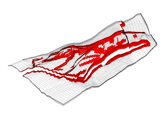
We then distinguish the active and inactive cells
cla;
plotGrid(G,find(~actnum(G.cells.indexMap)), 'FaceColor','none',pargs{:});
plotGrid(G,find( actnum(G.cells.indexMap)), 'FaceColor','y', pargs{:});
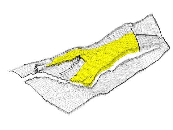
Show various subsets of the model
Prepare to extract a subgrid - show the part that will be extracted
clear ijk;
[ijk{1:3}] = ind2sub(G.cartDims, G.cells.indexMap(:));
ijk = [ijk{:}];
[I,J,K] = meshgrid(6:15, 80:100, 1:22);
cellNo = find (ismember(ijk, [I(:), J(:), K(:)], 'rows'));
a = actnum(G.cells.indexMap); in = find(a(cellNo));
plotGrid(G,cellNo(in),'FaceColor','m');
view(-186,68)
[I,J,K] = meshgrid(9:11, 65:67, 1:22);
cellNo = find (ismember(ijk, [I(:), J(:), K(:)], 'rows'));
plotGrid(G,cellNo,'FaceColor','r');
[I,J,K] = meshgrid(29:31, 55:75, 1:22);
cellNo = find (ismember(ijk, [I(:), J(:), K(:)], 'rows'));
plotGrid(G,cellNo,'FaceColor','b');
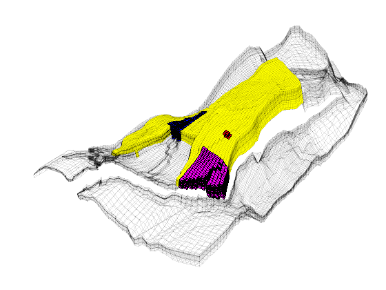
Extract the subgrid and compute pillars
grdecl.ACTNUM = actnum;
cut_grdecl = cutGrdecl(grdecl, [6 15; 80 100; 1 22]);
g = computeGeometry(processGRDECL(cut_grdecl));
figure
plotCellData(g,g.cells.volumes, pargs{:});
colormap(jet), brighten(.5)
axis tight off, view(210,15); zoom(1.2);
set(gca,'Clipping','off')
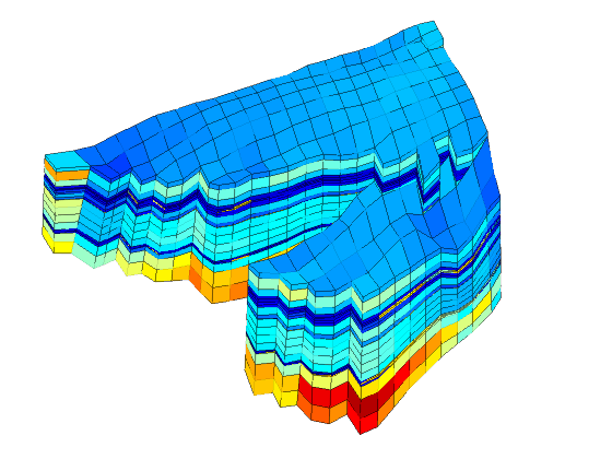
cut_grdecl = cutGrdecl(grdecl, [9 11; 65 67; 1 22]);
g = processGRDECL(cut_grdecl);
figure,
[X,Y,Z] = buildCornerPtPillars(cut_grdecl,'Scale',true);
[x,y,z] = buildCornerPtNodes(cut_grdecl);
plot3(X',Y',Z','-k',x(:),y(:),z(:),'or');
plotGrid(g);
axis tight off, view(180,20);
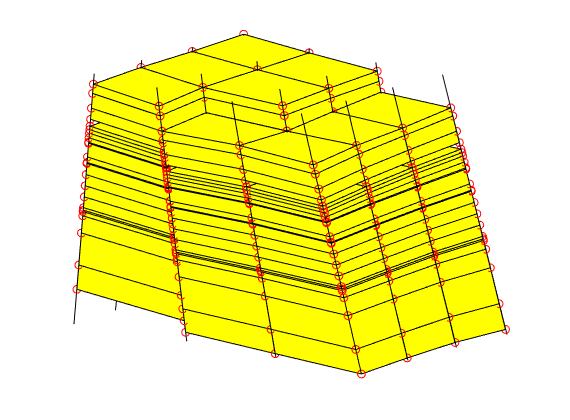
cut_grdecl = cutGrdecl(grdecl, [29 31; 55 75; 1 22]);
g = processGRDECL(cut_grdecl);
figure,
plotGrid(g);
plotFaces(g,find(g.faces.tag>0),'FaceColor','b','EdgeColor','b','FaceAlpha',.5);
axis tight off, view(180,27); zoom(1.2); camdolly(0,-0.2,0)
set(gca,'Clipping','off')
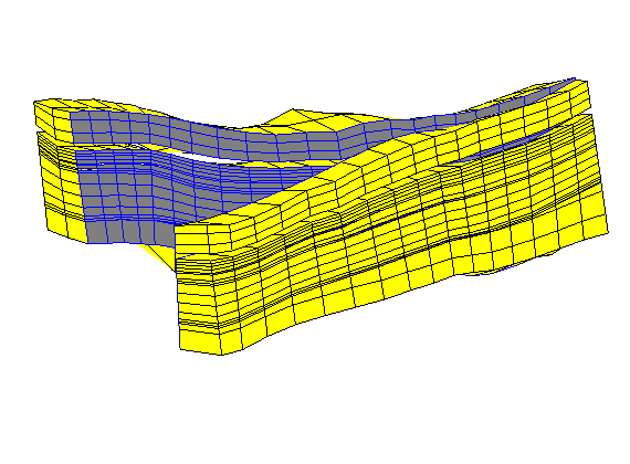
Extract the active part of the model
To get the whole grid, we need to reprocess the input data. This gives a grid with two components: the main reservoir and a detached stack of twelve cells, which we ignore henceforth.
G = processGRDECL(grdecl);
clf
plotGrid(G(1),pargs{:});
plotGrid(G(2),pargs{:},'FaceColor','r');
view(-110,50), axis tight off, set(gca,'DataAspect',[20 11 1]); zoom(1.7);
set(gca,'Clipping','off')
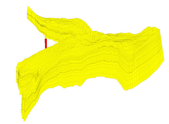
Outline petrophysical properties
The petrophysical properties are included in the simulation model subset represented by function makeNorneSubsetAvailable. Consequently, the necessary data has been read into the grdecl structure. We can then extract the petrophysical properties. Notice that here, the rock
close all, G = G(1);
rock = grdecl2Rock(grdecl, G.cells.indexMap);
Porosity First, we show the porosities as they are generated on a Cartesian grid that corresponds to geological ‘time zero’, i.e., an imaginary time at which all the depositional layers were stacked as horizontally on a Cartesian grid.
p = reshape(grdecl.PORO, G.cartDims);
clf
slice(p, 1, 1, 1); view(-135,30), shading flat,
axis equal off, set(gca,'ydir','reverse','zdir','reverse')
colorbarHist(p(p(:)>0), [.05 .35],'South',100);
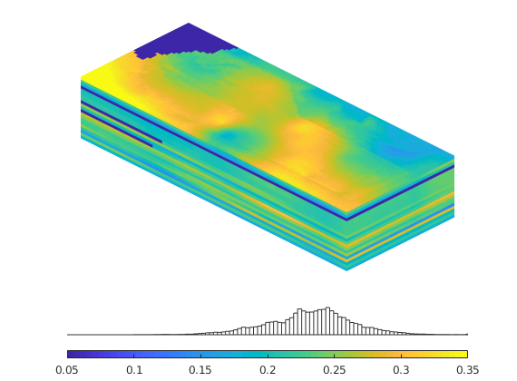
Then we show the porosities mapped onto the structural grid
clf
plotCellData(G,rock.poro, pargs{:});
axis tight off; set(gca,'DataAspect',[2 1 0.1]);
view(-110,55); zoom(1.8);
colorbarHist(rock.poro, [.05 .35],'South',100);
set(gca,'Clipping','off')
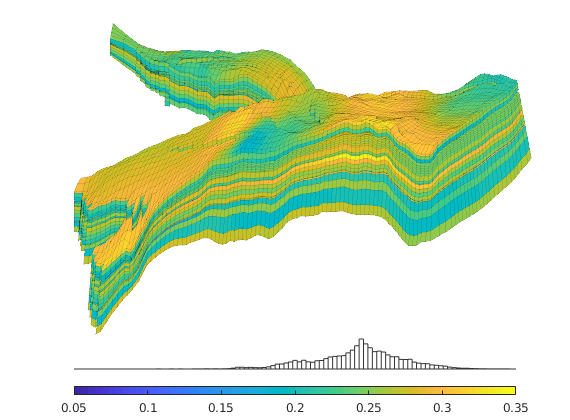
show also the net-to-gross
clf
plotCellData(G,rock.ntg, pargs{:});
axis tight off; set(gca,'DataAspect',[1 1 0.1]);
view(-110,55); zoom(1.8);
colorbarHist(rock.ntg,[.05 1],'South',100);
set(gca,'Clipping','off')
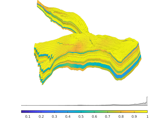
Permeability The permeability is generally a tridiagonal tensor K = diag(Kx, Ky, Kz). For the Norne model, the data file only specifies Kx, and then various manipulations are done to get the correct vertical permeability.
clf
p = log10(rock.perm(:,3));
plotCellData(G,p, pargs{:});
axis tight off; set(gca,'DataAspect',[1 1 0.1]);
view(-110,55); zoom(1.8);
set(gca,'Clipping','off')
% Manipulate the colorbar to get the ticks we want
cs = [1 10 100 1000 10000];
caxis(log10([min(cs) max(cs)]*milli*darcy));
hc = colorbarHist(p(~isinf(p)),caxis,'South',100);
set(hc, 'YTick', 0.5, 'YTickLabel','mD', ...
'XTick', log10(cs*milli*darcy), 'XTickLabel', num2str(cs'));
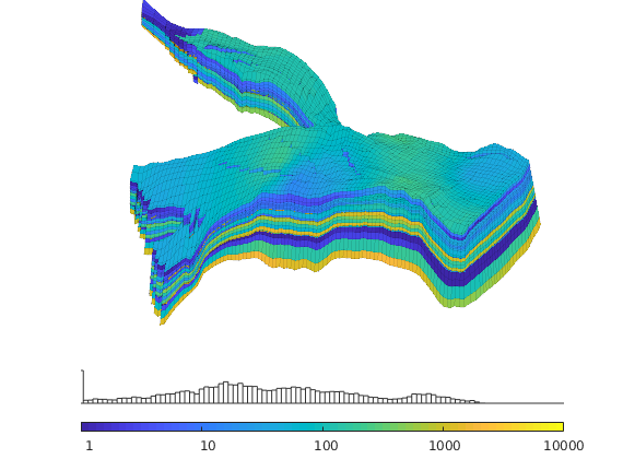
clf
p = log10(rock.perm(:,3));
plotCellData(G,p, pargs{:});
axis tight off; set(gca,'DataAspect',[1 1 0.1]);
view(-110,55); zoom(1.8);
set(gca,'Clipping','off')
% Manipulate the colorbar to get the ticks we want
cs = [0.1 1 10 100 1000];
caxis(log10([.1 2500]*milli*darcy));
hc = colorbarHist(p(~isinf(p)),caxis,'South',100);
set(hc, 'YTick', 0.5, 'YTickLabel','mD', ...
'XTick', log10(cs*milli*darcy), 'XTickLabel', num2str(cs'));
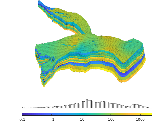
<html>
% <p><font size="-1
Introduction to the SAIGUP Model
Generated from showSAIGUP.m
In this example, we will examine a model from the project Sensitivity Analysis of the Impact of Geological Uncertainties on Production forecasting in clastic hydrocarbon reservoirs (SAIGUP). The model has faults, inactive cells, and disconnected components, but no pinchout. We will show how to read, process, and visualize the reservoir model and discuss some of the petrophysical properties.
Read and process the model
We start by reading the model from a file in the Eclipse format (GRDECL) that can be read using the readGRDECL function. (If the model is not available the getDatasetPath function will download and install it for you).
grdecl = fullfile(getDatasetPath('SAIGUP'), 'SAIGUP.GRDECL');
grdecl = readGRDECL(grdecl);
Error using input
Cannot call INPUT from EVALC.
Error in downloadDataset>confirm_download (line 184)
response = input(prompt, 's');
Error in downloadDataset>do_download (line 163)
do_get = confirm_download(info);
...
MRST uses the strict SI conventions in all of its internal calculations. The SAIGUP model, however, is provided using the ECLIPSE ‘METRIC’ conventions (permeabilities in mD and so on). We use the functions getUnitSystem and convertInputUnits to assist in converting the input data to MRST’s internal unit conventions.
usys = getUnitSystem('METRIC');
grdecl = convertInputUnits(grdecl, usys);
grdecl %#ok (intentional display)
From the output of readGRDECL, we see that the file contains four fields:
Since the keyword ACTNUM is present, the model is likely to contain both active and inactive cells. To be able to plot both the active and the inactive cells, we need to override the ACTNUM field when processing the input, because if not, the inactive cells will be ignored when the unstructured grid is built. We generate a space-filling geometry using the processGRDECL function
actnum = grdecl.ACTNUM;
grdecl.ACTNUM = ones(prod(grdecl.cartDims),1);
G = processGRDECL(grdecl, 'Verbose', true, 'checkgrid', false);
WARNING: inactive cells often contain garbage data and should generally not be inspected in this manner. Here, most inactive cells are defined in a reasonable way. By not performing basic sanity checks on the resulting grid (option 'checkgrid'=false), we manage to process the grid and produce reasonable graphical output. In general, however, we strongly advice that 'checkgrid' remain set in its default state of true.
To simplify the processing, a single layer of artificial cells is added above the top and below the bottom of the model, but not touching the model. (See the tutorial “Read, Display, and Manipulate” for more details). In the following, we therefore work with a 40x120x22 model.
In the first phase, we process all faces with normals in the logical i-direction. There should be 40x120x22=105600, out of which 96778 are not degenerate or at a fault. In the next phase, we process the faults and split faces to obtain a matching grid. Here there are faults at 521 pairs of pillars and the splitting of these results in 27752 new faces. If each face were split in two, we would have obtained 521x(20x2+2)=21882, which means that some of the faces have been split into at least three subfaces. The process is then repeated in the logical j-direction.
The processing assumes that there are no faults in the logical k-direction and therefore processes only regular connections. In absence of inactive or pinched cells, there should be (20+1+4)x120x40=120000 faces (where +4 is due to the artificial cells) in the k-direction. The result of the grid processing is a new structure G, outlined below
G %#ok (intentional display)
Inspect the whole model
Having obtained the grid in the correct unstructured format, we first plot the outline of the whole model and highlight all faults. This model consist of two separated grids so that numel(G)=2
newplot; subplot('position',[0.025 0.025 0.95 0.95]);
for i=1:numel(G)
plotGrid(G(i),'FaceColor','none','EdgeColor',[0.65 0.65 0.65], ...
'EdgeAlpha',0.2);
plotFaces(G(i),find(G(i).faces.tag>0),'FaceColor','red','EdgeAlpha',0.1);
end
axis off; view(-10,40); camdolly(0,-0.2,0)
Then we distinguish the active and inactive cells using the 'FaceColor' property set to 'none' for the inactive cells and to 'y' for the active cells. We notice that that only G(1) has active cells, this is indicated with the warning.
cla;
for i=1:numel(G)
hi = plotGrid(G(i),find(~actnum(G(i).cells.indexMap)), ...
'FaceColor','none','EdgeColor',[0.65 0.65 0.65],'EdgeAlpha',0.2);
ha = plotGrid(G(i),find( actnum(G(i).cells.indexMap)), ...
'FaceColor','y','EdgeAlpha',0.1);
end
axis off; view(-15,20); camdolly(0,-0.2,0); axis normal
Inspect the active model
To inspect only the active model, we reset the ACTNUM field to its original values and recreate the grid. Now, inactive cells will be ignored and we therefore get a different unstructured grid. If we include the actnum, G from proccessGRDECL has only one component.
grdecl.ACTNUM = actnum; clear actnum;
G = processGRDECL(grdecl);
clf,
pargs = {'EdgeAlpha'; 0.1; 'EdgeColor'; 'k'};
plotGrid(G, pargs{:}); view(-100,40); axis tight off
Once the active part of the model is read, we can compute geometric primitives like cell and face centroids, cell areas, and face centroids and normals by means of the computeGeometry function.
G = computeGeometry(G);
clf
plotCellData(G,G.cells.centroids(:,3), pargs{:});
view(-100,40); axis tight off
The media (rock) properties can be extracted by means of the grdecl2Rock function. This function inspects the keywords present in the input data and constructs a rock data structure that holds the permeability tensor
(in the structure field
perm), possibly porosity values(in the
porofield).
The first input argument is the raw input data as constructed by function readGRDECL. The second, optional, input argument is a list of active cells represented as a mapping from the grid’s cells to the global grid cells from the original Nx-by-Ny-by-Nz box description. WARNING: the grdecl2Rock routine returns permeability values in units [md] and to use the rock structure for simulation, we therefore need to convert the permeabilities to SI units. This was done by the function convertInputUnits when we first read the data.
rock = grdecl2Rock(grdecl, G.cells.indexMap);
Porosity
The porosity data are given with one value for each cell in the model. First, we show the porosities as they are generated on a Cartesian grid that corresponds to geological ‘time zero’, i.e., an imaginary time at which all the depositional layers were stacked as horizontally on a Cartesian grid.
p = reshape(grdecl.PORO, G.cartDims);
clf
slice(p, 1, 1, 1); view(-135,30), shading flat,
axis equal off, set(gca,'ydir','reverse','zdir','reverse')
colorbarHist(grdecl.PORO, [.01 .3],'South',100);
Then we show the porosities mapped onto the structural grid
clf
plotCellData(G,rock.poro, pargs{:});
axis tight off; set(gca,'DataAspect',[1 1 0.1]);
view(-65,55);
colorbarHist(rock.poro, [.01 .3],'South',100);
show also the net-to-gross
clf
plotCellData(G,rock.ntg, pargs{:});
axis tight off; set(gca,'DataAspect',[1 1 0.1]);
view(-65,60);
colorbarHist(rock.ntg,[.2 1],'South',100);
and the satnum
clf
SN = grdecl.SATNUM(G.cells.indexMap); j = jet(60);
plotCellData(G,SN, pargs{:});
axis tight off; set(gca,'DataAspect',[1 1 0.1]);
view(-65,60);
colorbarHist(SN, [.5 6.5], 'South', 0:.5:6.5);
colormap(j(1:10:end,:))
and a plot where we split them up
clf
plotGrid(G,'FaceColor','none', pargs{:});
axis tight off; set(gca,'DataAspect',[1 1 0.1]);
view(-65,60);
caxis([0.5 6.5]), colormap(j(1:10:end,:))
h1 = plotCellData(G,SN, find(SN==1), pargs{:});
h2 = plotCellData(G,SN, find(SN==5), pargs{:});
delete([h1,h2])
h1 = plotCellData(G,SN, find(SN==2), pargs{:});
h2 = plotCellData(G,SN, find(SN==4), pargs{:});
delete([h1,h2])
h1 = plotCellData(G,SN, find(SN==3), pargs{:});
h2 = plotCellData(G,SN, find(SN==6), pargs{:});
Permeability
The permeability is given as a tridiagonal tensor K = diag(Kx, Ky, Kz) and we therefore plot each of the horizontal and vertical components using a logarithmic color scale. The vertical permeability has a large number of zero values. These are shown as dark blue color, but are not included in the histogram
close
for i=[1,3]
figure;
p = log10(rock.perm(:,i));
plotCellData(G,p, pargs{:});
axis tight off; set(gca,'DataAspect',[1 1 0.1]);
view(-65,55);
% Manipulate the colorbar to get the ticks we want
cs = [0.001 0.01 0.1 1 10 100 1000 10000];
caxis(log10([min(cs) max(cs)]*milli*darcy));
hc = colorbarHist(p(~isinf(p)),caxis,'South',100);
set(hc, 'YTick', 0.5, 'YTickLabel','mD', ...
'XTick', log10(cs*milli*darcy), 'XTickLabel', num2str(cs'));
colormap(jet)
end
Likewise, we show a combined histogram of the horizontal/vertical permeability (with all zero values excluded).
figure
Kx = convertTo(rock.perm(:,1),milli*darcy);
Kz = convertTo(rock.perm(:,3),milli*darcy);
hist(log10(Kx),100);
hold on
hist(log10(Kz(Kz>0)),100);
hold off
h=get(gca,'Children');
set(h(1),'EdgeColor',[0 0 0.4],'FaceColor','none')
set(h(2),'EdgeColor',[0.6 0 0],'FaceColor','none')
h = legend('Horizontal','Vertical'); set(h,'FontSize',16);
and one histogram per rock type
figure('Position',[0 60 900 350]);
col = jet(60); col=col(1:10:end,:);
for i=1:6,
subplot(2,3,i);
hist(log10(Kx(SN==i)), 100);
h = findobj(gca,'Type','patch');
set(h,'FaceColor',col(i,:),'EdgeColor',col(i,:))
set(gca,'XLim',[-3 4],'XTick',-2:2:4,'XTickLabel',num2str(10.^(-2:2:4)'));
end
Finally, show the multiplicator values
figure
Mx = grdecl.MULTX(G.cells.indexMap);
My = grdecl.MULTY(G.cells.indexMap);
Mz = grdecl.MULTZ(G.cells.indexMap);
plotGrid(G,'FaceColor','none','EdgeAlpha',0.1);
plotCellData(G,Mz,Mz<1,pargs{:});
axis tight off; set(gca,'DataAspect',[1 1 0.1]);
view(-65,55);
colorbarHist(Mz(Mz<1),[0 1],'South',100);
Copyright notice
<html>
% <p><font size="-1
Model 2 of the 10th SPE Comparative Solution Project
Generated from showSPE10.m
The data set was originally posed as a benchmark for upscaling methods. The 3-D geological model consists of 60x220x85 grid cells, each of size 20ftx10ftx2ft. The model is a geostatistical realization from the Jurassic Upper Brent formations, in which one can find the giant North Sea fields of Statfjord, Gullfaks, Oseberg, and Snorre. In this specific model, the top 70 ft (35 layers) represent the shallow-marine Tarbert formation and the lower 100 ft (50 layers) the fluvial Ness formation. The data can be obtained from the SPE website: http://www.spe.org/web/csp/ The data set is used extensively in the literature, and for this reason, MRST has a special module that will download and provide easy access to the data set. In this example, we will inspect the SPE10 model in more detail.
mrstModule add spe10
Load the model
The first time you access the model, the MRST dataset system will prompt you to download the model from the official website of the comparative solution project. Depending upon your internet connection this may take quite a while–even several minutes–so please be patient. Notice that getSPE10rock returns permeabilities in strict SI units (i.e., m^2), and the petrophysical data of this model may therefore be used directly in simulations in MRST.
rock = getSPE10rock();
p = reshape(rock.poro,60,220,85);
Kx = reshape(log10(rock.perm(:,1)),60,220,85) - log10(milli*darcy);
Ky = reshape(log10(rock.perm(:,2)),60,220,85) - log10(milli*darcy);
Kz = reshape(log10(rock.perm(:,3)),60,220,85) - log10(milli*darcy);
Attempting to download 'SPE10' dataset (48.1 MB)...
Successfully downloaded dataset.
show p
clf
slice( p, [1 220], 60, [1 85]);
shading flat, axis equal, set(gca,'zdir','reverse'), box on;
set(gca,'XTick',[],'YTick',[],'ZTick',[]);
colorbarHist(p(:),[-.01 max(p(:))],'South',100);
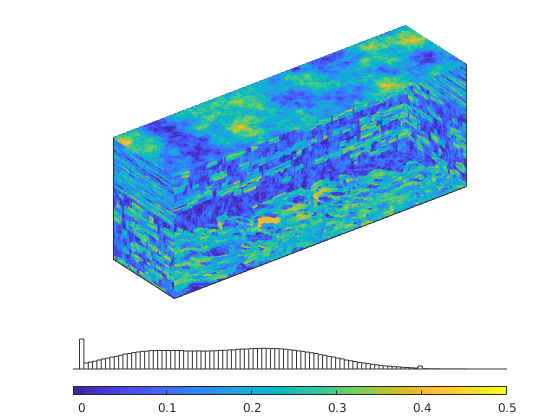
show Kx/Ky
These are identical so we only plot one of them
clf
slice( Kx, [1 220], 60, [1 85]);
shading flat, axis equal, set(gca,'zdir','reverse'), box on;
set(gca,'XTick',[],'YTick',[],'ZTick',[]);
h=colorbarHist(Kx(:), caxis, 'South', 100);
set(h,'XTickLabel',10.^get(h,'XTick'));
set(h,'YTick',mean(get(h,'YLim')),'YTickLabel','mD');
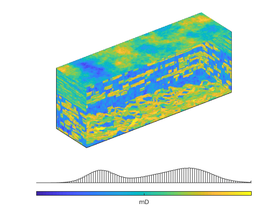
show Kz
clf
slice( Kz, [1 220], 60, [1 85]);
shading flat, axis equal, set(gca,'zdir','reverse'), box on;
set(gca,'XTick',[],'YTick',[],'ZTick',[]);
h=colorbarHist(Kz(:), caxis, 'South', 100);
set(h,'XTickLabel',10.^get(h,'XTick'));
set(h,'YTick',mean(get(h,'YLim')),'YTickLabel','mD');
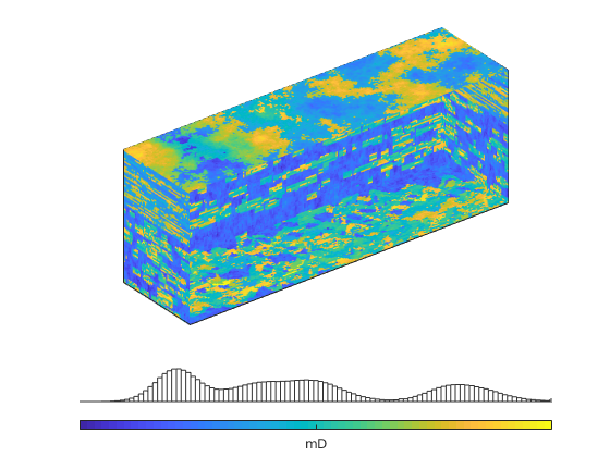
show horizontal permeability distributions
clf
hist(Kx(220*60*35+1:end),101);
hold on
hist(Kx(1:220*60*35),101)
hold off
h=get(gca,'Children');
set(h(1),'EdgeColor',[0 0 0.4],'FaceColor','none')
set(h(2),'EdgeColor',[0.7 0 0],'FaceColor','none')
h=legend('Ness','Tarbert'); set(h,'FontSize',16);
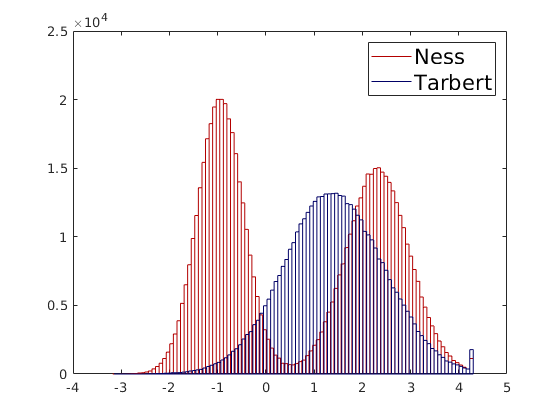
show vertical permeability distributions
clf;
hist(Kz(1:220*60*35),101)
hold on
hist(Kz(220*60*35+1:end),101);
hold off
h=get(gca,'Children');
set(h(2),'EdgeColor',[0 0 0.4],'FaceColor','none')
set(h(1),'EdgeColor',[0.7 0 0],'FaceColor','none')
h=legend('Tarbert','Ness');set(h,'FontSize',16);
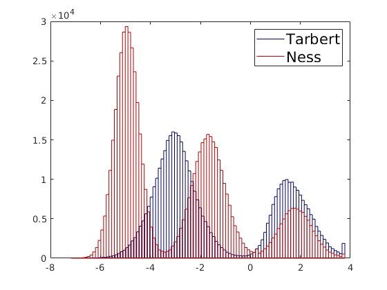
show porosity distributions
T = p(1:220*60*35); pN = p(220*60*35+1:end);
pb = linspace(0,0.5,101);
N=histc(pN,pb); bar(pb,N,'histc');
hold on
N=histc(pT,pb); bar(pb,N,'histc');
hold off;
h=get(gca,'Children');
set(h(1),'EdgeColor',[0 0 0.4],'FaceColor','none')
set(h(2),'EdgeColor',[0.7 0 0],'FaceColor','none')
h=legend('Ness','Tarbert');set(h,'FontSize',16);
set(gca,'XLim',[0 0.5]);
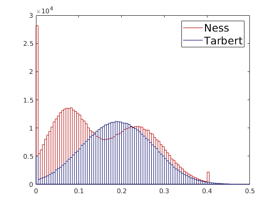
How to Read, Display, and Manipulate Corner-Point Grids
Generated from gridTutorialCornerPoint.m
In this example we will show several examples how to manipulate and plot corner-point data. As an example, we will use a family of simple models with a single fault, which can be realized in different resolutions.
Creating and visualizing a small realization of the model
We start by generating an input stream in the Eclipse format (GRDECL) for a 2x1x2 realization of the model
grdecl = simpleGrdecl([2, 1, 2], 0.15) %#ok (intentional display)
grdecl =
struct with fields:
cartDims: [2 1 2]
COORD: [36×1 double]
ZCORN: [32×1 double]
...
From the output of simpleGrdecl, we see that the file contains four fields:
The next step is to process this input stream to build the structure for the grid, which here will be represented in a fully unstructured format. To simplify the processing, a single horizontal layer of artifical cells is added one length unit above the top and below the bottom of the model, but not touching the model. (This is what is reported in the first line of the output). In the following, we therefore work with a 2x1x4 model, as shown in the folowing figure
Process the grid
G = processGRDECL(grdecl, 'Verbose', true); clear grdecl;
Adding 4 artificial cells at top/bottom
Processing regular i-faces
Found 8 new regular faces
Elapsed time is 0.010503 seconds.
Processing i-faces on faults
Found 1 faulted stacks
...
In the first phase, we process all faces with normals in the logical i-direction. Altogether, there should be 3x1x4=12 faces. As we see from the figure, there is fault along the second pair of pillars in the i-direction. Therefore, only 8 of the 12 faces are reported as regular faces. In the next phase of the processing, we treat all pillars pairs (fault stacks) that contain at least one set of non-matching z-coordinates. Here, there is one such stack and two cells that have a non-matching connection. After having split the non-matching faces, the stack contains 7 faces (including one face for each of the artificial layers) that are added to the list of faces. Then the process is repeated in the logical j-direction, in which there are only matching faces. The processing assumes that there are no faults in the logical k-direction and therefore processes only regular connections. In absence of inactive or pinched cells, there should be (2+5)x1x2=14 faces. Finally, the four artifical cells are removed and the routine correctly reports that there are no inactive cells. The result of the grid processing is a new structure G, outlined below
G %#ok (intentional display)
G =
struct with fields:
type: {'processGRDECL'}
griddim: 3
nodes: [1×1 struct]
...
More information about the grid structure can be found in the documentation. After the successful processing, we plot the outline of the model and mark the faulted faces
clf, subplot('position',[0.025 0.025 0.95 0.95])
plotGrid(G,'FaceColor','b','FaceAlpha', 0.1);
plotFaces(G,find(G.faces.tag>0),'FaceColor','red');
axis equal off, view(40,15)
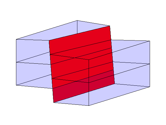
Setting inactive cells
In this section, we will work with a slightly larger model realization and show how one can manipulate the model by setting inactive cells. To this end, we start by creating the input stream and building the grid structure
grdecl = simpleGrdecl([30, 20, 5], 0.12);
G = processGRDECL(grdecl);
The resulting model has a single fault and layers given by sinusoidal surfaces. First, we plot the outline of the model and mark all fault faces in red color
cla
plotGrid(G,'FaceColor','none','EdgeColor',[0.65 0.65 0.65]);
h = plotFaces(G,find(G.faces.tag>0),'FaceColor','red');
axis tight off, view(65,40)
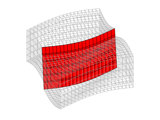
Then we restrict the model to be inside an ellipse in the logical (i,j) coordinates with the principal axis in the i-direction. The model is restricted by setting all cells with centerpoint in (i,j)-coordinates outside the ellipsis as inactive.
[j,i] = meshgrid(linspace(-0.95,0.95,G.cartDims(2)), ...
linspace(-0.95,0.95,G.cartDims(1)) );
actnum = ones(G.cartDims(1:2));
actnum( (i.^2/4 + j.^2)>0.5) = 0;
actnum = reshape(repmat(actnum,[1 1 G.cartDims(3)]),[],1); clear i j;
set(h, 'FaceAlpha', 0.3);
plotGrid(G,find( actnum(G.cells.indexMap)),'FaceColor','y');
view(20,30), clear h
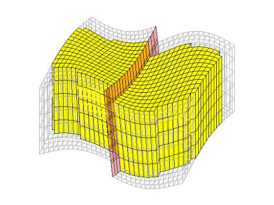
To get rid of the inactive cells, we process the model again and plot the result to see that it is correct
grdecl.ACTNUM = actnum; clear actnum
G = processGRDECL(grdecl); clear grdecl
cla
plotGrid(G);
axis tight off, view(20,30)
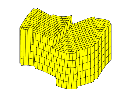
Visualizing the layered structure
To better visualize the layered structure of the model, we plot the scalar field ‘val(i,j,k)=k’ over the grid. This field is constructed using the logical Cartesian dimensions of the model, and then the values corresponding to the active cells are extracted using ‘G.cells.indexMap’.
cla,
val = ones(G.cartDims(1:3));
val = cumsum(val,3);
plotCellData(G,val(G.cells.indexMap),'EdgeColor','k');
clear val
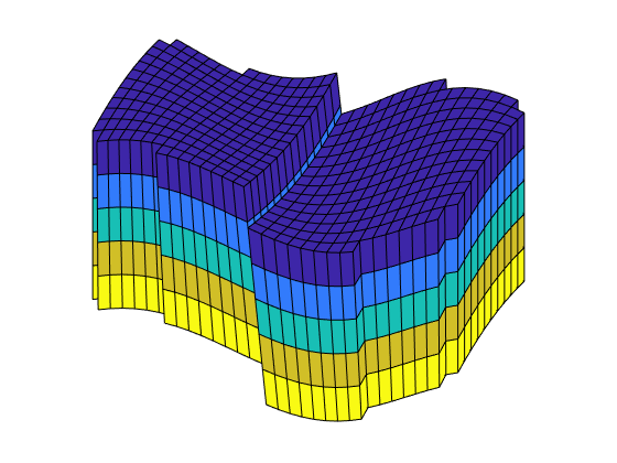
Visualizing individual cells
As our first example, we extract and visualize all cells that are neighbor to a fault. To this end, we pick all rows in ‘G.faces.neighbors’ that correspond to faces that are marked as faults, i.e., has a positive value for ‘G.faces.tag’. If a cell has more than one fault faces, this cell will appear more then once in the list. Moreover, outer fault faces will be characterized by one of the cell numbers being zero. Before we can plot the faces, we must therefore remove redundancy and zero cell numbers.
cellList = G.faces.neighbors(G.faces.tag>0, :);
cells = unique(cellList(cellList>0));
cla,
plotGrid(G,'FaceColor','none','EdgeColor',[0.65 0.65 0.65]);
plotGrid(G,cells);
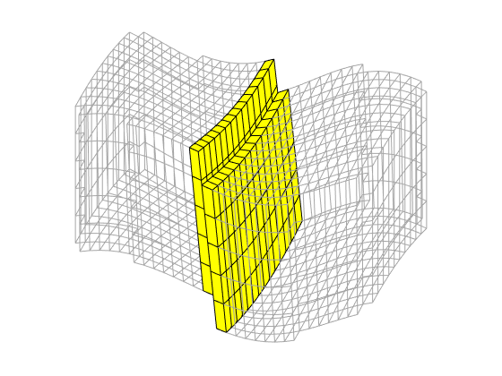
Similarly, we can also plot all cells that are neighbors to internal fault faces by first removing all rows in cellList that have one zero entry
cellList = cellList(all(cellList>0,2),:);
cells = unique(cellList(cellList>0));
plotGrid(G,cells,'FaceColor','g');
clear cellList cells
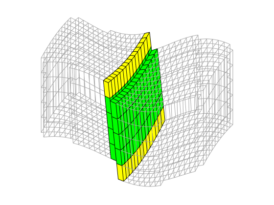
Using ijk-subscripts to access cells
In the second example, we demonstrate how one can use the logical structure of the corner-point grid to pick all active cells corresponding to the logical index map [1:2:end,:,1:end/2] and color them using the i-value. To be able to access the grid using (i,j,k) adressing, we must first construct the subscript values ‘ijk’ from the linear index ‘G.cells.indexMap’ using the builtin function ‘ind2sub’.
% Plot grid outline
cla
plotGrid(G,'FaceColor','none','EdgeColor',[0.65 0.65 0.65]);
% Compute the subindex
clear ijk
[ijk{1:3}] = ind2sub(G.cartDims, G.cells.indexMap);
ijk = [ijk{:}];
% Exctract all active cells for subscript values [1:2:end,:,1:end/2]
[J,K]=meshgrid(1:G.cartDims(2),1:G.cartDims(3)/2);
col = ['b','r','g','c','m','y','w'];
for i=1:2:G.cartDims(1)
cellNo = find(ismember(ijk, [repmat(i,[numel(J),1]), J(:), K(:)],'rows'));
plotGrid(G,cellNo,'FaceColor',col(mod(i,numel(col))+1));
end
%clear J K cellNo ijk col
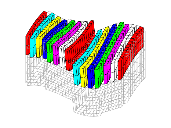
Creating a coarse partitioning
Base on the fine-grid model, we will now create a 5x4x3 coarse partitioning with an uneven partitioning in the vertical direction. To this end, we will use functionality from the coarsegrid module.
mrstModule add coarsegrid
nz = G.cartDims(3);
blockIx = partitionLayers(G,[5 4], ceil([1 nz/2 nz nz+1]));
cla
plotCellData(G,mod(blockIx,8),'EdgeColor','k');
outlineCoarseGrid(G,blockIx, 'FaceColor', 'none', 'LineWidth', 2);
axis tight off, view(20,30)
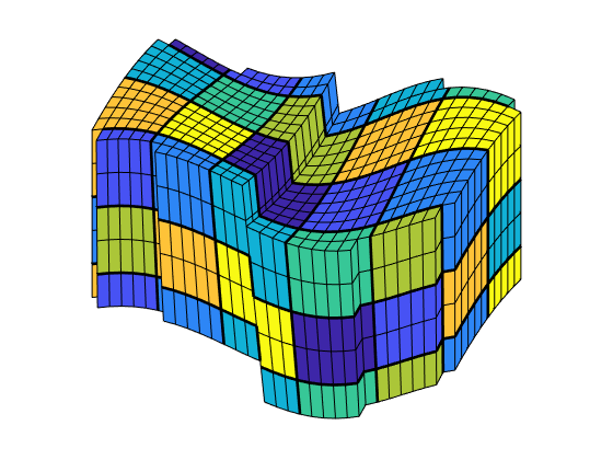
Because the partitioning has been performed in logical index space, we have so far disregarded the fact the some of the blocks may contain disconnected cells because of erosion, faults, etc. Here we see that the coarse blocks with indices [3,:,:] do not consist of a single set of connected cells. We therefore postprocess the grid to split disconnected blocks in two.
blockIx = processPartition(G,blockIx);
cla
plotCellData(G,mod(blockIx,8),'EdgeColor','k');
outlineCoarseGrid(G,blockIx, 'FaceColor', 'none', 'LineWidth', 2);
axis tight off, view(20,30)
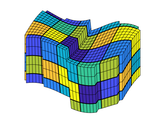
From the plot above, it is not easy to see the shape of the individual coarse blocks. We therefore first highlight three representative blocks.
blocks = [4, 6, 28];
col = ['b', 'r', 'g', 'c', 'm', 'y'];
cla
plotGrid(G, 'EdgeColor', [0.75, 0.75, 0.75], 'FaceColor', 'w')
outlineCoarseGrid(G, blockIx, 'FaceColor', 'none', 'LineWidth', 2)
for i = 1 : numel(blocks),
plotGrid(G, blockIx == blocks(i), ...
'FaceColor', col(mod(i, numel(col)) + 1));
end
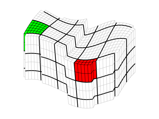
Alternatively, we can view the partitioning using explosionView, which moves all blocks out a certain distance from the centerpoint of the model.
cla
G = computeGeometry(G);
explosionView(G,blockIx,.5), view(30,50); axis tight off
colormap(colorcube(max(blockIx)))
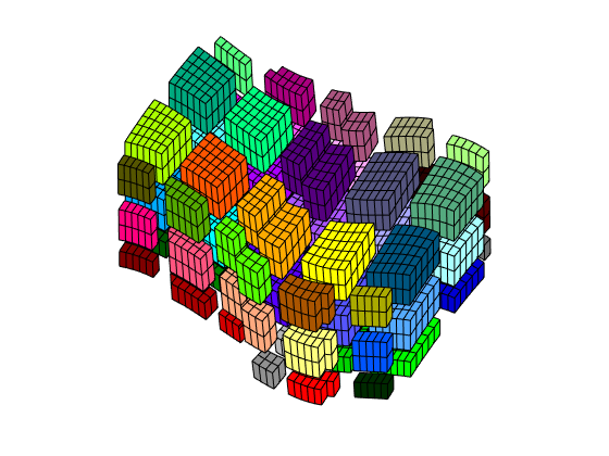
Build the coarse-grid
Having obtained a partition we are satisfied with, we build the coarse-grid structure. This structure consists of three parts:
CG = generateCoarseGrid(G, blockIx);
CG %#ok (intentional display)
CG.cells % (intentional display)
CG.faces % (intentional display)
CG =
struct with fields:
cells: [1×1 struct]
faces: [1×1 struct]
partition: [1940×1 double]
...
Let us now use CG to inspect some of the blocks in the coarse grid. To this end, we arbitrarily pick a few blocks and inspect these block and their neighbours. For the first block, we plot the cells but do not highlight the faces that have been marked as lying on a fault
cla
plotBlockAndNeighbors(CG, blocks(1), 'PlotFaults', false([2, 1]))
view(30, 50), axis tight, colormap(jet)
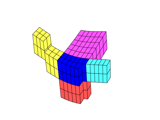
The next block lies at a fault, so therefore we highlight the fault faces as well
cla
plotBlockAndNeighbors(CG, blocks(3), 'PlotFaults', true([2, 1]))
view(20, 30)
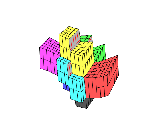
<html>
% <p><font size="-1
Overview of Grid Factory Routines
Generated from gridTutorialIntro.m
In this tutorial, we will introduce you briefly to the grid structure and give an overview of some of the many grid factory routines that can be used to generate various types of grids.
Create a 2D grid
We start by creating a simple 2D Cartesian grid. We then remove one cell and add geometry information to the resulting grid.
G = cartGrid([3,2]);
G = removeCells(G, 2);
G = computeGeometry(G);
% Plot the grid
newplot
plotGrid(G,'FaceColor',[0.95 0.95 0.95]); axis off;
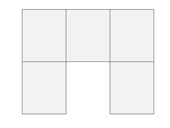
Plot cell, face, and node numbers
MRST uses a fully unstructured grid format in which cells, faces, and nodes, as well as their topological relationships, are represented explicitly. To illustrate, we extract the cell and face centroids as well as the coordinates of each node. These will be used for plotting the cells, faces and node indices, respectively.
c_cent = G.cells.centroids;
f_cent = G.faces.centroids;
coords = G.nodes.coords;
% Add circles around the centroids of each cell
hold on;
pltarg = {'MarkerSize',20,'LineWidth',2,'MarkerFaceColor',[.95 .95 .95]};
plot(c_cent(:,1), c_cent(:,2),'or',pltarg{:});
% Plot triangles around face centroids
plot(f_cent(:,1), f_cent(:,2),'sg',pltarg{:});
% Plot squares around nodes
plot(coords(:,1), coords(:,2),'db',pltarg{:});
legend({'Grid', 'Cell', 'Face', 'Node'}, 'Location', 'SouthOutside', 'Orientation', 'horizontal')
% Plot cell/face centroids and nodes
txtargs = {'FontSize',12,'HorizontalAlignment','left'};
text(c_cent(:,1)-0.04, c_cent(:,2), num2str((1:G.cells.num)'),txtargs{:});
text(f_cent(:,1)-0.045, f_cent(:,2), num2str((1:G.faces.num)'),txtargs{:});
text(coords(:,1)-0.075, coords(:,2), num2str((1:G.nodes.num)'),txtargs{:});
title('Grid structure')
hold off;
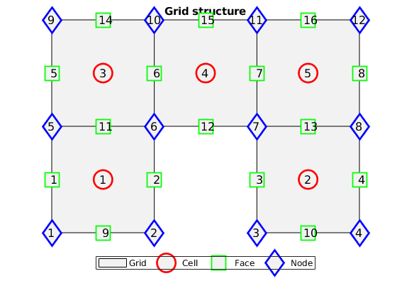
Finding mappings between grid primitives
The unstructured grid is built upon coordinates representing nodes, nodes representing faces and faces representing cells. To save memory, some attributes are run length encoded. For more information, see ‘help grid_structure’. For instance, let us look up information for the faces.
faces =[ rldecode(1 : G.cells.num,diff(G.cells.facePos), 2).' G.cells.faces];
tag = {'West'; 'East'; 'South'; 'North'; 'Bottom'; 'Top'};
fprintf('Cell\tFace\tTag id\tTag\n');
for i=1:size(faces,1)
fprintf(' %3d\t%3d\t%3d\t[%s]\n', faces(i,1:3), tag{faces(i,3)});
end
Cell Face Tag id Tag
1 1 1 [West]
1 9 3 [South]
1 2 2 [East]
1 11 4 [North]
2 3 1 [West]
2 10 3 [South]
2 4 2 [East]
...
Neighborship is defined through faces
G.faces.neighbors(i,:) contains the cells neighboring to face i. We define a new grid and plot the neighbors of face 10 in the new grid.
clf;
plotGrid(G,'FaceAlpha', 1, 'FaceColor', [0.95 0.95 0.95]); axis off;
f = 6;
plotGrid(G, G.faces.neighbors(f,:), 'FaceColor', 'Green')
text(f_cent(f,1)-0.1, f_cent(f,2), num2str(f),'FontSize',16,'Color','red');
% This also defines the boundary faces, since faces with only one neighbor
% is on the edge of the domain:
boundary = any(G.faces.neighbors==0,2);
facelist = 1:G.faces.num;
fprintf('Boundary faces: \n')
facelist( boundary) %#ok intentional display
fprintf('Internal faces: \n')
facelist(~boundary) %#ok intentional display
Boundary faces:
ans =
1 2 3 4 5 8 9 10 12 14 15 16
Internal faces:
...
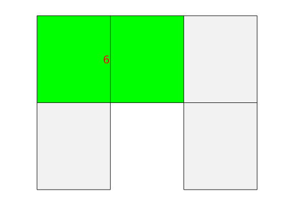
Generating synthethic grids using MRST
There are many options for creating synthethic grids in MRST. For instance, the simple cartGrid already shown is a special case of tensorGrid:
G = tensorGrid((1:10).^3, 1:5);
clf;
plotGrid(G);
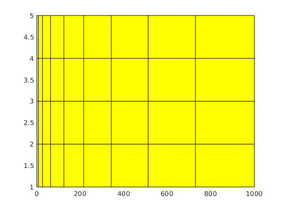
Triangulated grids
We can generate a triangulated grid using existing triangulations, from MATLAB or elsewhere.
% Generate points
pts = rand(20,3).*repmat([10,10,1], 20, 1);
% Triangulate
T = delaunayn(pts);
G = tetrahedralGrid(pts, T);
clf, title('Tetrahedral grid')
plotGrid(G);
view(50,60), axis tight off
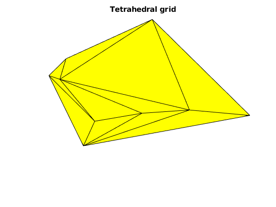
Triangular grids
Generate a 2D triangle grid from the same data using the xy-coordinates
pts_2d = pts(:,1:2);
% Triangulate
T = delaunay(pts_2d(:,1), pts_2d(:,2));
G_tri = triangleGrid(pts_2d, T);
clf, title('Triangular grid')
plotGrid(G_tri); axis tight off
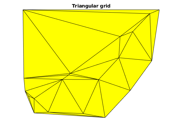
Extruded grid
If we have an interesting 2D grid, we can easily extend it to 3D by using makeLayeredGrid. We will extend the previous triangle grid to 3 layers
G = makeLayeredGrid(G_tri, 3);
clf;
title('Extruded triangular grid')
plotGrid(G);
view(50,60), axis tight off
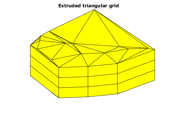
Explicit hexahedral grid
Hexahedral grids can also be generated by lists of nodes and node indices. For valid node ordering, see help hexahedralGrid
H = [1 2 3 4 5 6 7 8; ...
% Cell 1
2 9 10 3 6 11 12 7]; ...
% Cell 2
P = [ 1 0 0.1860; ...
1 1 0.1852; ...
1 1 0.1926; ...
1 0 0.1930; ...
0 0 0.1854; ...
0 1 0.1846; ...
0 1 0.1923; ...
0 0 0.1926; ...
1 2 0.1844; ...
1 2 0.1922; ...
0 2 0.1837; ...
0 2 0.1919]; ...
G = hexahedralGrid(P, H);
clf;
plotGrid(G);
axis tight
view(40,40)
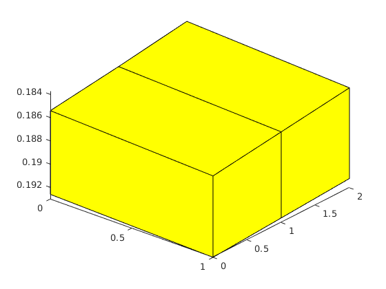
Grids can be manipulated after creation
We can alter the attributes of a grid after creation. In this example we twist the grid slightly. One caveat: Any computed properties of the grid will not be altered. This means that computeGeometry must be called again after grid updates to get correct centroids, volumes, normals, etc.
G = cartGrid([10, 10]);
G_before = computeGeometry(G);
% Twist the coordinates to create a non-K-orthogonal grid.
G_after = twister(G);
G_after = computeGeometry(G_after);
clf;
plotGrid(G_after);
hold on
plot(G_before.cells.centroids(:,1), G_before.cells.centroids(:,2), 'Or')
plot(G_after.cells.centroids(:,1), G_after.cells.centroids(:,2), 'xb')
legend('Twisted grid', 'Original centroids', 'Modified centroids', ...
'Location', 'NorthOutside', 'Orientation', 'horizontal')
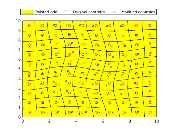
Some grid routines produce corner-point input data
Corner-point grids are usually represented on a special format given in ECLIPSE input files. MRST have a few routines that generate special grid models given on this input format, which in turn can be converted to MRST grids using processGRDECL, just as one would with a GRDECL file read using readGRDECL. For instance, here is a three layered structure which is easy to generate by creating pillars manually.
G = processGRDECL( threeLayers(10,10,5));
G = computeGeometry(G);
clf;
% Color the cells by the cell volume to show the layered structure.
plotCellData(G, G.cells.volumes,'EdgeColor','k');
view(120,10);
axis tight off
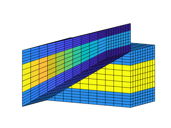
Grids generated by simpleGrdecl
The function simpleGrdecl can generate different example grids based on optional parameters. The default parameter gives a simple, wavy grid.
grdecl = simpleGrdecl([20, 20, 5]);
G1 = processGRDECL(grdecl);
clf, plotGrid(G1), view(3), axis tight off;
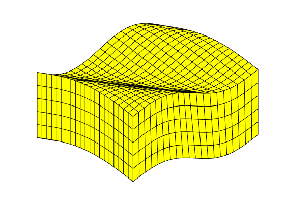
By supplying a function handle, the grid becames faulted based on the values of the function at the fault line.
grdecl = simpleGrdecl([20, 20, 5], @(x) 0.05 * (sin(2*pi*x) - 1.5));
G2 = processGRDECL(grdecl);
clf, plotGrid(G2), view(3), axis tight off;
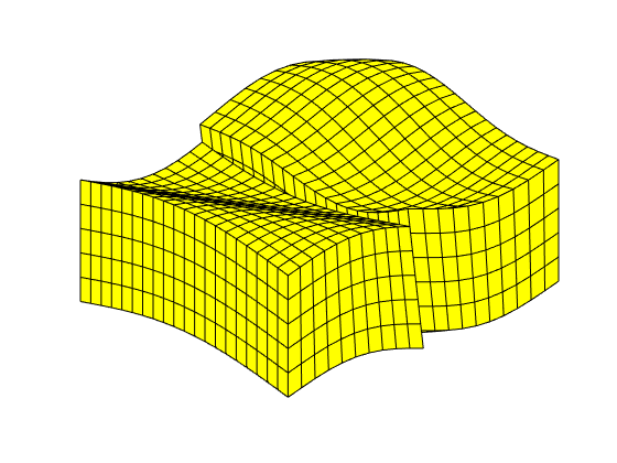
Create a flat grid with another fault function
grdecl = simpleGrdecl([20, 20, 5], @(x) 0.25*(x-0.5), 'flat', true);
G3 = processGRDECL(grdecl);
clf, plotGrid(G3), view(3), axis tight off;
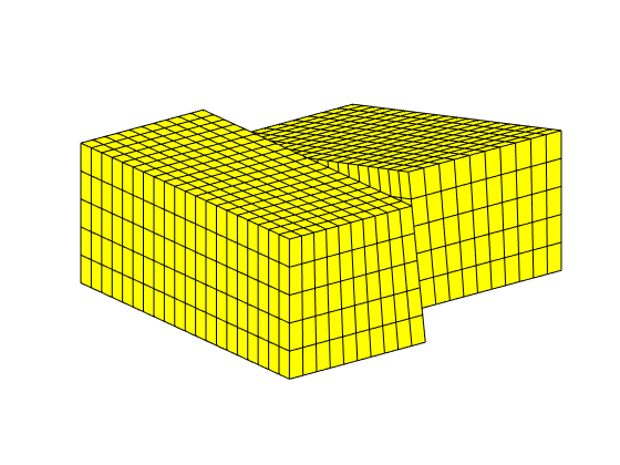
<html>
% <p><font size="-1
Basic Grid Tutorial: Rectilinear/Curvilinear Grids
Generated from gridTutorialStruct.m
In this tutorial, we describe how you can use MRST to construct Cartesian and rectilinear grids for rectangular and non-rectangular domains and show how you can populate your grid with petrophysical properties. To this end, we will grid a rectangular domain, from which we cut out a half circle. This example is discussed in more detail in Jolt 2
Tensor grid
clf
dx = 1 - 0.5*cos((-1:0.1:1)*pi);
x = -1.15 + 0.1*cumsum(dx);
y = 0:0.05:1;
G = tensorGrid(x, y.^0.75);
plotGrid(G, 'FaceColor', 'none');
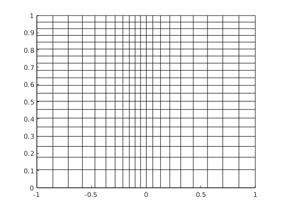
Compute geometry
disp('G.cells = '); disp(G.cells)
G = computeGeometry(G);
disp('G.cells = '); disp(G.cells)
cla, plotCellData(G, G.cells.volumes);
G.cells =
num: 400
facePos: [401×1 double]
indexMap: [400×1 double]
faces: [1600×2 double]
G.cells =
num: 400
...
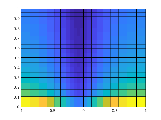
Define indicator for circular sector
r = sqrt(sum(G.cells.centroids .^ 2, 2));
cla, plotCellData(G, double(r > 0.6));
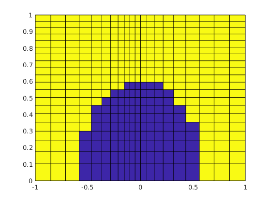
Extract subgrid
disp('G.cells = '); disp(G.cells)
Gs = extractSubgrid(G, r > 0.6);
disp('Gs.cells = '); disp(Gs.cells)
cla, plotGrid(Gs, 'FaceColor', 'none');
G.cells =
num: 400
facePos: [401×1 double]
indexMap: [400×1 double]
faces: [1600×2 double]
volumes: [400×1 double]
centroids: [400×2 double]
...
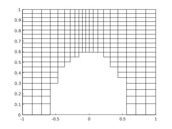
Generate permeability
K = convertFrom(logNormLayers([G.cartDims, 1], 1), milli*darcy);
rock.perm = reshape(K(Gs.cells.indexMap), [], 1);
cla, plotCellData(Gs, rock.perm);

Perturbe inner nodes
fI = false([Gs.faces.num, 1]);
fI(boundaryFaces(Gs)) = true;
nI = true([Gs.nodes.num, 1]);
n = mcolon(Gs.faces.nodePos(fI), Gs.faces.nodePos(fI) + 1);
nI(Gs.faces.nodes(n)) = false;
Gs.nodes.coords(nI,:) = Gs.nodes.coords(nI,:) + 0.007*randn([sum(nI), 2]);
cla, plotCellData(Gs, rock.perm);
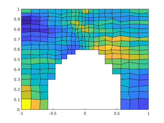
Copyright Notice
Basic Grid Operations and Manipulations: Rectilinear/Curvilinear Grids
Generated from gridTutorialUnstruct.m
In this tutorial, we describe how you can use MRST to construct various kinds of unstructured grids based on Delaunay triangulations and Voronoi diagrams. This example is discussed in more detail in Jolt 2
Triangular grid in 2D
clf
[x,y] = meshgrid(0:10,0:8);
x(2:8,2:10) = x(2:8,2:10) + .25*randn(7,9);
y(2:8,2:10) = y(2:8,2:10) + .25*randn(7,9);
G = triangleGrid([x(:) y(:)]);
h=plotGrid(G,'FaceColor','none');
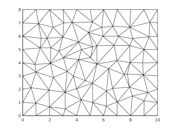
Voronoi diagram
V = pebi(G);
hold on, plot(x(:),y(:),'k.','MarkerSize',12); hold off
plotGrid(V,'FaceColor','none','LineWidth',2);
delete(h)
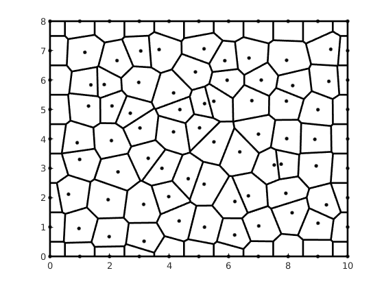
Standard data set from Matlab
load seamount;
plot(x(:),y(:),'k.','MarkerSize',12);
t = delaunay(x(:), y(:));
G = triangleGrid([x(:) y(:)], t);
plotGrid(G,'FaceColor','none');
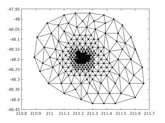
Extrude to 3D
G = makeLayeredGrid(G,5);
clf
plotGrid(G,'FaceColor',[1 .8 .8]); view(5,45); axis tight off
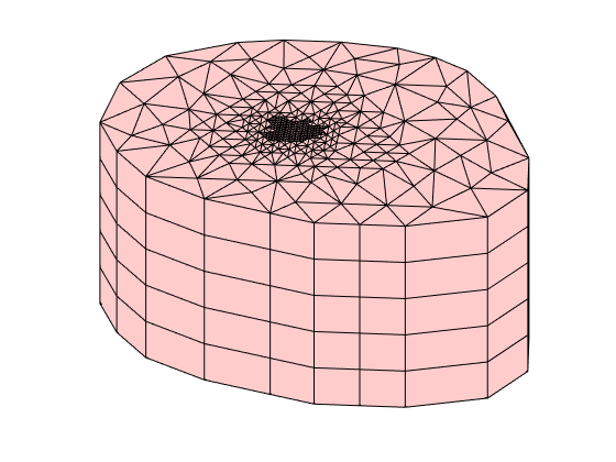
Radial grid
P = [];
for r = exp(-3.5:0.25:0),
[x,y,z] = cylinder(r,16); P = [P [x(1,:); y(1,:)]]; %#ok<AGROW>
end
[x,y] = meshgrid(-2.5:2.5,-2.5:2.5);
P = unique([P'; x(:) y(:); 0 0],'rows');
G = makeLayeredGrid(pebi(triangleGrid(P)), 3);
cla, plotGrid(G,'FaceColor',[1 .8 .8]); view(30,60), axis tight off
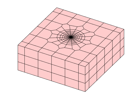
Cartesian grid with radial refinement
Pw = [];
for r = exp(-3.5:.2:0),
[x,y,z] = cylinder(r,28); Pw = [Pw [x(1,:); y(1,:)]];
end
Pw = [Pw [0; 0]];
Pw1 = bsxfun(@plus, Pw, [2; 2]);
Pw2 = bsxfun(@plus, Pw, [12; 6]);
[x,y] = meshgrid(0:.5:14, 0:.5:8);
P = unique([Pw1'; Pw2'; x(:) y(:)], 'rows');
G = pebi(triangleGrid(P));
cla, plotGrid(G,'FaceColor','none'); axis([-.1 14.1 -.1 8.1]); axis off
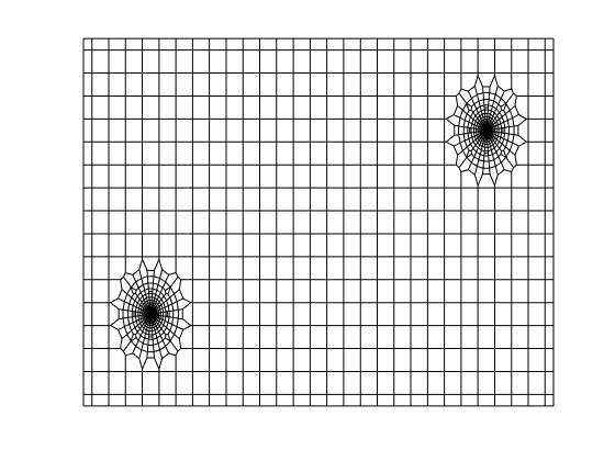
Copyright notice
<html>
% <p><font size="-1