`solvent`: Solvent solvers¶

Models¶

Base classes¶

Contents¶

MODELS

Files: BlackOilSolventModel - Black-oil solvent model. equationsBlackOilSolvent - Generate linearized problem for the black-oil solvent model equations

class BlackOilSolventModel(G, rock, fluid, varargin)¶

Bases: ThreePhaseBlackOilModel

Black-oil solvent model.

getActivePhases(model)¶: Get active flag for the canonical phase ordering (water, oil gas as on/off flags).

getPhaseIndices(model)¶: Get the active phases in canonical ordering

getPhaseNames(model)¶: Get the active phases in canonical ordering

storeDensity(model, state, rhoW, rhoO, rhoG, rhoS)¶: Store compressibility / surface factors for plotting and output.

storeFluxes(model, state, vW, vO, vG, vS)¶: Utility function for storing the interface fluxes in the state

storeMobilities(model, state, mobW, mobO, mobG, mobS)¶: Utility function for storing the mobilities in the state

storeUpstreamIndices(model, state, upcw, upco, upcg, upcs)¶: Store upstream indices, so that they can be reused for other purposes.

storebfactors(model, state, bW, bO, bG, bS)¶: Store compressibility / surface factors for plotting and output.

hystereticResSat = None¶: Dynamic end-point scaling should be used in a proper solvent model,

solvent = None¶: HC residual saturations can be set to the smallest observed over the entire

equationsBlackOilSolvent(state0, state, model, dt, drivingForces, varargin)¶

Generate linearized problem for the black-oil solvent model equations

Synopsis:

[problem, state] = equationsBlackOilSolvent(state0, state, model, dt, drivingForces)

Description:

This is the core function of the black-oil solvent model. This function assembles the residual equations for the conservation of water, oil and gas, as well as required well equations. By default, Jacobians are also provided by the use of automatic differentiation.

The model assumes two extrema: In cases with only oil, reservoir gas and water, we have traditional black-oil behavior. In cases with oil, solvent gas and water, the oil mixes with the solvent gas according to the Todd-Longstaff model. In intermediate regions, we interpolate between the two extrema based on the solvet to total gas saturation fraction, and the pressure.

Keyword Arguments:
Parameters:	state0 – Reservoir state at the previous timestep. Assumed to have physically reasonable values. state – State at the current nonlinear iteration. The values do not need to be physically reasonable. model – BlackOilSolventModel-derived class. Typically, equationsBlackOil will be called from the class getEquations member function. dt – Scalar timestep in seconds. drivingForces – Struct with fields: * W for wells. Can be empty for no wells. * NOTE: The current implementation does not support BC’s and sources.
	‘Verbose’ – Extra output if requested. ‘reverseMode’ – Boolean indicating if we are in reverse mode, i.e. solving the adjoint equations. Defaults to false. ‘resOnly’ – Only assemble residual equations, do not assemble the Jacobians. Can save some assembly time if only the values are required. ‘iterations’ – Nonlinear iteration number. Special logic happens in the wells if it is the first iteration.
Returns:	problem – LinearizedProblemAD class instance, containing the water, oil and gas conservation equations, as well as well equations specified by the FacilityModel class. state – Updated state. Primarily returned to handle changing well controls from the well model.

Utilities¶

Contents¶

UTILS

Files: addSolventProperties - Add solvent pseudo-component and properties to fluid. computeFlashBlackOilSolvent - Compute flash for a black-oil solvent model with disgas/vapoil computeRelPermSolvent - Calulates effective relative permeabilities. computeResidualSaturations - Calculate effective residual saturations computeViscositiesAndDensities - Calculates effective viscosities and densities using Todd-Longstaff getFluxAndPropsSolvent - Flux and other properties for the black-oil solvent model equations. getPlotAfterStepSolvent - Get a function that allows for dynamic plotting in simulateScheduleAD makeWAGschedule - Make schedule for water-alternating gas (WAG) injection. plotSolventFluidProps - Terneary plots of HC components in black-oil solvent model.

addSolventProperties(fluid, varargin)¶: Add solvent pseudo-component and properties to fluid.

computeFlashBlackOilSolvent(state, state0, model, status)¶

Compute flash for a black-oil solvent model with disgas/vapoil

Synopsis:

state = computeFlashBlackOil(state, state0, model, status)

Description:

Compute flash to ensure that dissolved properties are within physically reasonable values, and simultanously avoid that properties go far beyond the saturated zone when they were initially unsaturated and vice versa.

Parameters:	state – State where saturations, rs, rv have been updated due to a Newton-step. state0 – State from before the linearized update. model – The ThreePhaseBlackOil derived model used to compute the update. status – Status flags from getCellStatusVO, applied to state0.
Returns:	state – Updated state where saturations and values are chopped near phase transitions.

Note

Be mindful of the definition of state0. It is not necessarily the state at the previous timestep, but rather the state at the previous nonlinear iteration!

computeRelPermSolvent(model, p, sW, sO, sG, sS, sWcon, sOr, sGc, mobMult)¶: Calulates effective relative permeabilities.

computeResidualSaturations(model, p, sW, sG, sS, state0)¶: Calculate effective residual saturations

computeViscositiesAndDensities(model, p, sW, sO, sG, sS, sOr, sGc, rs, rv, isSatO, isSatG)¶: Calculates effective viscosities and densities using Todd-Longstaff model + 1/4th-power mixing rule

getFluxAndPropsSolvent(fluid, pO, krW, krO, krG, krS, muW, muO, muG, muS, rhoW, rhoO, rhoG, rhoS, sW, sG, sS, T, gdz, op)¶: Flux and other properties for the black-oil solvent model equations.

getPlotAfterStepSolvent(state0, model, varargin)¶: Get a function that allows for dynamic plotting in simulateScheduleAD for the black-oil solvent model.

See also

getPlotAfterStep

makeWAGschedule(W, nCycles, varargin)¶

Make schedule for water-alternating gas (WAG) injection.

Synopsis:

schedule = makeWAGschedule(W, nCycles)

Description:

This function makes a WAG schedule based on a well structure, to be used with the BlackOilSolventModel.

Keyword Arguments:
Parameters:	W – Well structure, properly initialized with e.g. addWell(). The function assumes this is initialized with desired rates/bhp. nCycles – Number of cycles.
	‘time’ – Total duration of the WAG injection period. Defaults to 1 year. ‘dt’ Target time step size. Defaluts to 30 days. ‘gas_end’ – Duration of gas injection, 0 < gas_end < 1. The gas injection period of each cycle will last for time/ncyclegas_end. Defaults to 0.5. ‘useRampUp’* – Use rampup each time the well control changes to ease the nonlinear solution process. Defaults to false.
Returns:	schedule – WAG injection schedule.

Examples¶

Using the black-oil solvent model¶

Generated from solventExample1D.m

In this example, we investigate black-oil solvent model, which models the effect of injecting a solvent gas that mixes with the reservoir hydrocarbon fluids. The model is an extension of the Todd-Longstaff mixing model, which treats the solvent gas as a fourth pseudo-component.

mrstModule add ad-core ad-props ad-blackoil spe10 mrst-gui solvent

df = get(0, 'defaultfigureposition');
close all

Set up grid and rock¶

We will set up a simple 1D example with homogeneous rock properties

n = 50;
l = 100*meter;
G = computeGeometry(cartGrid([n,1,1], [l,1,1]));

perm = 100*milli*darcy;
poro = 0.4;
rock = makeRock(G, perm, poro);

Set up fluid and add solvent gas properties¶

The solvent model we will use, treats solvent gas as a fourth pseudocomponent, which is either miscible or immiscible with the oil and gas, depending on the fraction of solvent concentration to total gas concentration,

, and the pressure. The model assumes one immiscible and one miscible residual saturation for the hydrocarbon phases, with

, and we must define both. In this example, we assume that the critical (residual) gas saturation is zero in both the immiscible and miscible case. The degree of mixing is modeled through a mixing paramter

that defines the degree of mixing, where (no mixing)

(full mixing).

% Set up three-phase fluid with quadratic relperms
fluid = initSimpleADIFluid('n'     , [2, 2, 2]                        , ...
                           'rho'   , [1000, 800, 100]*kilogram/meter^3, ...
                           'phases', 'WOG'                            , ...
                           'mu'    , [1, 3, 0.4]*centi*poise          );

sOr_i = 0.30; % Immiscible residual oil saturation
sOr_m = 0.10; % Miscible residual oil saturation
sGc_i = 0.15; % Immiscible residual oil saturation
sGc_m = 0.05; % Miscible residual oil saturation

% We scale the relperms to the immiscible endpoints
fluid.krW = coreyPhaseRelpermAD(2, 0    , fluid.krW(1 - (sOr_i + sGc_i)), sOr_i + sGc_i);
fluid.krG = coreyPhaseRelpermAD(2, sGc_i, fluid.krG(1 - sOr_i), sOr_i + sGc_i);
[fluid.krO, fluid.krOW, fluid.krOG] ...
     = deal(coreyPhaseRelpermAD(2, sOr_i, fluid.krO(1 - sGc_i), sOr_i + sGc_i));

% Add the solvent pseudocomponent to the fluid
fluid   = addSolventProperties(fluid, 'rhoSS' , 90*kilogram/meter^3, ...
                                      'muS'   , 0.5*centi*poise    , ...
                                      'mixPar', 1                  , ...
                                      'sOr_m' , sOr_m              , ...
                                      'sGc_m' , sGc_m              );

Set up black-oil solvent model¶

Since the residual saturations changes with the solvent and pressure, dynamic endpoint-scaling should be used in the relperm evaluations. However, this is somewhate unstable in cases where the initial oil or gas saturation is close to the residual saturation, and is thus disabeled by default.

model_fm = BlackOilSolventModel(G, rock, fluid                   , ...
                                       'extraStateOutput'      , true, ...
                                       'dynamicEndPointScaling', true);

Inspect fluid model¶

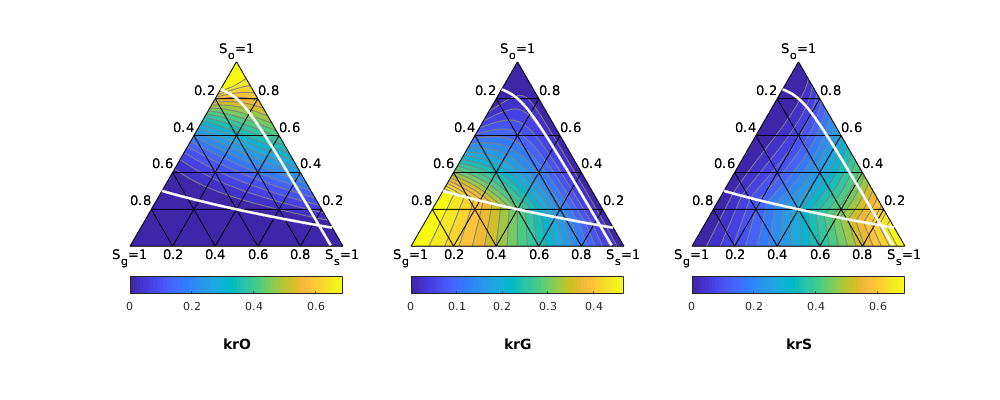
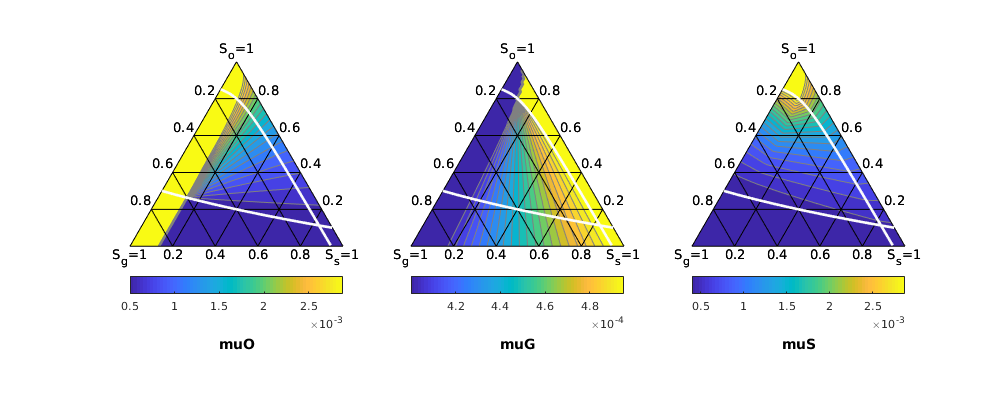
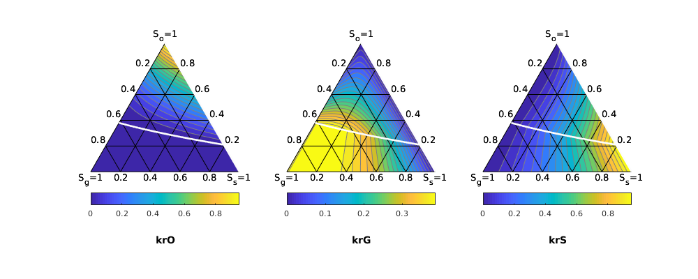
In regions with only oil, reservoir gas and water, we have traditional black-oil behavior, whereas regions with only water, reservoir oil and solvent gas, the oil is completely miscible with the solvent. In this case, solvent gas mixes with formation oil, effectively altering the viscosities, densities and relperms according the the Todd-Longstaff model [1]. In the intermediate region, we interpolate between the two extrema depending on the solvent to total gas saturation fraction, and the pressure. We look at terneary plots for the hydrocarbon relperms and viscosities when no water is present. Notice how the residual oil saturation (white line) reduces from

(immiscible) to

(miscible) with increasing solvent saturation, and the kinks in the gas and solvent relperms across this line.

plotSolventFluidProps(model_fm, {'kr', 'mu'}, {'O', 'G', 'S'});

Set up wells and simulate schedule¶

We set up a simple injection schedule where solvent is injected into the reservoir at constant rate over a period of three years. The reservoir is initially filled with a mixture of oil and water.

time = 3*year;
dt   = 30*day;
rate = 1*sum(poreVolume(G, rock))/time;
bhp  = 50*barsa;
W    = [];
W    = addWell(W, G, rock, 1          , 'type', 'rate', 'val', rate, 'comp_i', [0,0,0,1]);
W    = addWell(W, G, rock, G.cells.num, 'type', 'bhp' , 'val', bhp , 'comp_i', [1,0,0,0]);

tvec     = rampupTimesteps(time, dt);
schedule = simpleSchedule(tvec, 'W', W);

state0         = initResSol(G, 100*barsa, [0.6, 0.4, 0, 0]);
state0.wellSol = initWellSolAD(W, model_fm, state0);
[wellSols_fm, states_fm, reports_fm] = simulateScheduleAD(state0, model_fm, schedule);

Solving timestep 01/45:         -> 2 Hours, 2925 Seconds
Solving timestep 02/45: 2 Hours, 2925 Seconds -> 5 Hours, 2250 Seconds
Solving timestep 03/45: 5 Hours, 2250 Seconds -> 11 Hours, 900 Seconds
Solving timestep 04/45: 11 Hours, 900 Seconds -> 22 Hours, 1800 Seconds
Solving timestep 05/45: 22 Hours, 1800 Seconds -> 1 Day, 21 Hours
Solving timestep 06/45: 1 Day, 21 Hours -> 3 Days, 18 Hours
Solving timestep 07/45: 3 Days, 18 Hours -> 7 Days, 12 Hours
Solving timestep 08/45: 7 Days, 12 Hours -> 15 Days
...

Compare with moderate mixing¶

To see the effect of the mixing parameter

, we compare the results above with a model with moderate mixing, where we set

.

model_mm = model_fm;
model_mm.fluid.mixPar = 1/3;
[wellSols_mm, states_mm, reports_mm] = simulateScheduleAD(state0, model_mm, schedule);

Solving timestep 01/45:         -> 2 Hours, 2925 Seconds
Solving timestep 02/45: 2 Hours, 2925 Seconds -> 5 Hours, 2250 Seconds
Solving timestep 03/45: 5 Hours, 2250 Seconds -> 11 Hours, 900 Seconds
Solving timestep 04/45: 11 Hours, 900 Seconds -> 22 Hours, 1800 Seconds
Solving timestep 05/45: 22 Hours, 1800 Seconds -> 1 Day, 21 Hours
Solving timestep 06/45: 1 Day, 21 Hours -> 3 Days, 18 Hours
Solving timestep 07/45: 3 Days, 18 Hours -> 7 Days, 12 Hours
Solving timestep 08/45: 7 Days, 12 Hours -> 15 Days
...

Plot the results¶

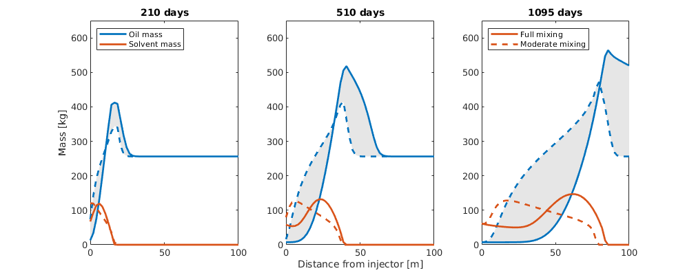
We now compare the results obtained from the two models by plotting the oil and solvent mass in each cell for three time steps. We see how the model with full mixing predicts a much higher oil recovery, and that the solvent travels faster with higher mixing due to the lower viscosity and thus higher mobility of the solvent-oil mixture. The difference in oil mass is shown as grey-shaded areas.

Plotting parameters
x      = linspace(0,l,n)';
phases = [2,4];
clr    = lines(numel(phases));
mrk    = {'-', '--'};
pargs  = @(phNo, mNo) {mrk{mNo}, 'color', clr(phNo,:), 'lineWidth', 2};
step   = [15, 25, 45];
pv     = model_fm.operators.pv;
gray   = [1,1,1]*0.9;
time   = cumsum(schedule.step.val);

% Residual oil mass in the immiscible and miscible case
massr_i = pv.*sOr_i*fluid.rhoOS;
massr_m = pv.*sOr_m*fluid.rhoSS;

% Mass of solvent and gas phase for each time step
getMass = @(states) cellfun(@(state) bsxfun(@times, pv, state.s(:,phases).*state.rho(:,phases)), ...
                                           states, 'uniformOutput', false);
mass = {getMass(states_fm); getMass(states_mm)};

figure('Position', [df(1:2), 1000, 400]);

for sNo = 1:numel(step)
    subplot(1, numel(step),sNo);
    box on; hold on
    for phNo = 1:numel(phases)
        if phases(phNo) == 2
                xx = [x; x(end:-1:1)];
                mm = [mass{1}{step(sNo)}(:, phNo);
                      mass{2}{step(sNo)}(end:-1:1, phNo)];
                fill(xx, mm, gray, 'edgecolor', 'none');
        end
        for mNo = 2:-1:1
            prg = pargs(phNo, mNo);
            [hm(mNo), hp(phNo)] = deal(plot(x, mass{mNo}{step(sNo)}(:,phNo), prg{:}));
        end
    end
    hold off
    if sNo == 1
        legend(hp, {'Oil mass', 'Solvent mass'}, 'Location', 'NorthWest')
        ylabel('Mass [kg]');
    elseif sNo == 2
        xlabel('Distance from injector [m]');
    elseif sNo == numel(step)
        legend(hm, {'Full mixing', 'Moderate mixing'}, 'Location', 'NorthWest')
    end
    ylim([0,650]);
    title([num2str(time(step(sNo))/day), ' days'])
end

Water-alternating Gas Injection in layer 10 of SPE10¶

Generated from spe10WAGexample.m

In this example, we simulate water-alternating gas injection (WAG) in a layer of SPE10 model 2, where we inject small volumes of water and solvent gas into the reservoir several cycles. The solvent gas mixes with the reservoir hydrocarbons according to a modified version of the Todd-Longstaff mixing model, which treats the solvent gas as fourth pseudocomponent.

mrstModule add ad-blackoil ad-props spe10 mrst-gui solvent

df = get(0, 'defaultfigureposition');
close all

Set up grid and rock properties¶

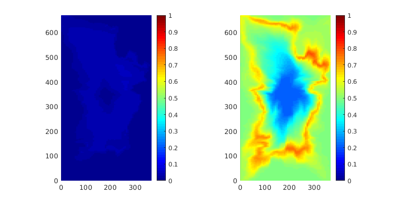
We pick up layer 10 of SPE10, and extract the grid and rock properties.

layers        = 10;
[~, model, ~] = setupSPE10_AD('layers', layers);
G             = model.G;
rock          = model.rock;

Set up fluid and add solvent gas properties¶

We will define our own fluid based on a three-phase fluid with water, oil and gas. The solvent model we will use, treats solvent gas as a fourth pseudocomponent, which is either miscible or immiscible with the oil and gas, depending on the fraction of solvent concentration to total gas concentration,

, and the pressure. The model assumes one immiscible and one miscible residual saturation for the hydrocarbon phases, with

. In this example, we assume that the critical (residual) gas saturation is zero in both the immiscible and miscible case. The model uses a mixing paramter

that defines the degree of mixing, where (no mixing) $ = 0 <= omega <= 1 = $ (full mixing).

fluid = initSimpleADIFluid('n'     , [2, 2, 2]                        , ...
                           'rho'   , [1000, 800, 100]*kilogram/meter^3, ...
                           'phases', 'WOG'                            , ...
                           'mu'    , [1, 3, 0.4]*centi*poise          , ...
                           'c'     , [1e-7, 1e-6, 1e-5]/barsa         );

sOr_i = 0.38; % Immiscible residual oil saturation
sOr_m = 0.21; % Miscible residual oil saturation

% We scale the relperms to the immiscible endpoints.
fluid.krW = coreyPhaseRelpermAD(2, 0, fluid.krG(1-sOr_i), sOr_i);
fluid.krG = coreyPhaseRelpermAD(2, 0, fluid.krG(1-sOr_i), sOr_i);
[fluid.krO, fluid.krOW, fluid.krOG] = deal(coreyPhaseRelpermAD(2, sOr_i, fluid.krO(1), sOr_i));

fluid = addSolventProperties(fluid, 'rhoSS' , 100*kilogram/meter^3, ...
                                      'mixPar', 2/3                 , ...
                                      'muS'   , 0.5*centi*poise     , ...
                                      'sOr_m' , sOr_m               , ...
                                      'c'     , 1e-5/barsa          );

% We use dynamic end-point scaling to account for the changes in residual
% saturaitons. This is disabeled by default since it can be somewhat
% unstable.
model4Ph = BlackOilSolventModel(G, rock, fluid, 'dynamicEndPointScaling', true);

Inspect fluid relperms¶

In regions with only oil, reservoir gas and water, we have traditional black-oil behavior, whereas regions with only water, reservoir oil and solvent gas, the oil is completely miscible with the solvent. In this case, solvent gas mixes with formation oil, effectively altering the viscosities, densities and relperms according the the Todd-Longstaff model. In the intermediate region, we interpolate between the two extrema depending on the solvent to total gas saturation fraction, and the pressure. We look at terneary plots for the hydrocarbon relperms of the hydrocardon phases when no water is present. Notice how the residual oil saturation (white line) reduces from

(immiscible) to

(miscible) with increasing solvent saturation.

plotSolventFluidProps(model4Ph, {'kr'}, {'O', 'G', 'S'});

Set up wells and injection schedule¶

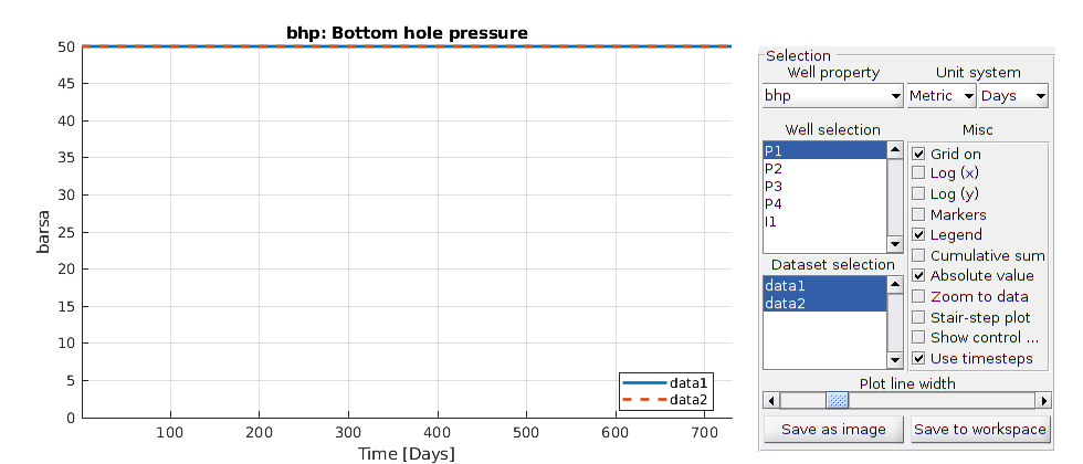
We consider the hello-world of reservoir simulation: A quarter-five spot pattern. The injector in the middle is operater at a fixed injection rate, while the producers in each corner is operated at a fixed bottom-hole pressure of 50 bars. During the first half year, we inject only water, while during the next year, we perform four cycles of equal periods of solvent gas and water injection. Finally, we perform half a year of water injection. This is a common strategy to reduce the growth of viscous fingers associated with gas injection, and uphold a more favourable injected to reservoir fluid mobility ratio.

timeW   = 0.5*year;                           % Duration of water injection periods
timeWAG = 2*timeW;                            % Duration of WAG period
rate    = 0.1*sum(poreVolume(G, rock))/timeW; % We inject a total of 0.4 PVI
bhp     = 50*barsa;                           % Producer bottom-hole pressure

producers = {1                                                     , ...
             G.cartDims(1)                                         , ...
             G.cartDims(1)*G.cartDims(2) - G.cartDims(1) + 1       , ...
             G.cartDims(1)*G.cartDims(2)                           };
injectors = {round(G.cartDims(1)*G.cartDims(2)/2 + G.cartDims(1)/2)};

W = [];
for pNo = 1:numel(producers)
    W = addWell(W, G, rock, producers{pNo}   , ...
                'type'  , 'bhp'              , ...
                'val'   , bhp                , ...
                'comp_i', [1,0,0,0]          , ...
                'sign'  , -1                 , ...
                'name'  , ['P', num2str(pNo)]);
end
for iNo = 1:numel(injectors)
    W = addWell(W, G, rock, injectors{iNo}     , ...
                'type'  , 'rate'               , ...
                'val'   , rate/numel(injectors), ...
                'comp_i', [1,0,0,0]            , ...
                'sign'  , 1                    , ...
                'name'  , ['I', num2str(iNo)]  );
end

dt1         = 60*day; % Timestep size for first water injection period
dt2         = 30*day; % Timestep size for WAG cycles and second water injection period
useRampUp   = true;   % We use a few more steps each time we change the
                      % well control to ease the nonlinear solution process
nCycles     = 4;      % Four WAG cycles
scheduleWAG = makeWAGschedule(W, nCycles, 'time'     , timeWAG  , ...
                                          'dt'       , dt2      , ...
                                          'useRampup', useRampUp);

tvec1                    = rampupTimesteps(timeW, dt1);
tvec2                    = rampupTimesteps(timeW, dt2, 0);
scheduleWAG.step.val     = [tvec1; scheduleWAG.step.val; tvec2];
scheduleWAG.step.control = [2*ones(numel(tvec1),1)  ; ...
                            scheduleWAG.step.control; ...
                            2*ones(numel(tvec2),1) ];

Define model and initial state, and simulate results¶

The reservoir is initially filled with a mixture of oil, reservoir gas and water. We set up a four-phase solvent model and simulate the schedule.

model4Ph.extraStateOutput = true;
sO = 0.5; sG = 0.4;
state0 = initResSol(G, 100*barsa, [1-sO-sG, sO, sG, 0]);
state0.wellSol = initWellSolAD(W, model4Ph, state0);

fn = getPlotAfterStepSolvent(state0, model4Ph, scheduleWAG, ...
                     'plotWell', true, 'plotReservoir', true);

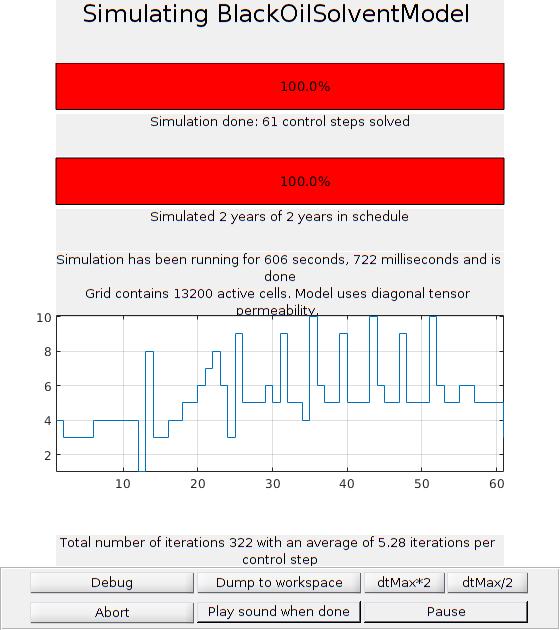
[wellSolsWAG, statesWAG, reportsWAG] ...
    = simulateScheduleAD(state0, model4Ph, scheduleWAG, 'afterStepFn', fn);

Solving timestep 01/61:         -> 5 Hours, 2250 Seconds
Solving timestep 02/61: 5 Hours, 2250 Seconds -> 11 Hours, 900 Seconds
Solving timestep 03/61: 11 Hours, 900 Seconds -> 22 Hours, 1800 Seconds
Solving timestep 04/61: 22 Hours, 1800 Seconds -> 1 Day, 21 Hours
Solving timestep 05/61: 1 Day, 21 Hours -> 3 Days, 18 Hours
Solving timestep 06/61: 3 Days, 18 Hours -> 7 Days, 12 Hours
Solving timestep 07/61: 7 Days, 12 Hours -> 15 Days
Solving timestep 08/61: 15 Days -> 30 Days
...

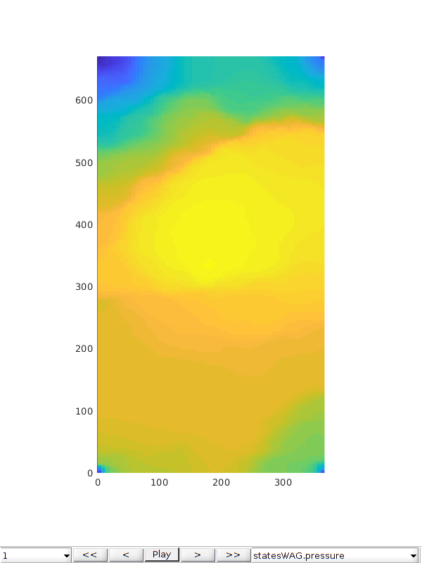
Interactive visualization of results¶

We use an interactive plotting tool to visualize reservoir results and the well solutions.

figure('Position', [df(1:2), 600,800])
plotToolbar(G, statesWAG); axis equal tight

Compare with standard water injection¶

We compare the results with standard water injection to see the effects of using WAG.

for wNo = 1:numel(W)
    W(wNo).compi = [1,0,0];
end

tvec     = rampupTimesteps(4*timeW, dt1);
schedule = simpleSchedule(tvec, 'W', W);
model3Ph = ThreePhaseBlackOilModel(G, rock, fluid);
model3Ph.extraStateOutput = true;
state0 = initResSol(G, 100*barsa, [1-sO-sG, sO, sG]);
state0.wellSol = initWellSolAD(W, model3Ph, state0);

[wellSol, states, reports] = simulateScheduleAD(state0, model3Ph, schedule);

Solving timestep 01/21:         -> 5 Hours, 2250 Seconds
Solving timestep 02/21: 5 Hours, 2250 Seconds -> 11 Hours, 900 Seconds
Solving timestep 03/21: 11 Hours, 900 Seconds -> 22 Hours, 1800 Seconds
Solving timestep 04/21: 22 Hours, 1800 Seconds -> 1 Day, 21 Hours
Solving timestep 05/21: 1 Day, 21 Hours -> 3 Days, 18 Hours
Solving timestep 06/21: 3 Days, 18 Hours -> 7 Days, 12 Hours
Solving timestep 07/21: 7 Days, 12 Hours -> 15 Days
Solving timestep 08/21: 15 Days -> 30 Days
...

Visulize well production curves¶

We look at the well production curves to see the difference of the two injection strategies.

lose all
tWAG = cumsum(scheduleWAG.step.val);
t    = cumsum(schedule.step.val);
for sNo = 1:numel(wellSol)
    [wellSol{sNo}.qSs] = deal(0);
end
plotWellSols({wellSolsWAG, wellSol},{tWAG, t})

solvent: Solvent solvers¶

Models¶

Base classes¶

Utilities¶

Examples¶

Using the black-oil solvent model¶

Set up grid and rock¶

Set up fluid and add solvent gas properties¶

Set up black-oil solvent model¶

Inspect fluid model¶

Set up wells and simulate schedule¶

Compare with moderate mixing¶

Plot the results¶

Water-alternating Gas Injection in layer 10 of SPE10¶

Set up grid and rock properties¶

Set up fluid and add solvent gas properties¶

Inspect fluid relperms¶

Set up wells and injection schedule¶

Define model and initial state, and simulate results¶

Interactive visualization of results¶

Compare with standard water injection¶

Visulize well production curves¶

`solvent`: Solvent solvers¶