`ad-mechanics`: Coupled flow and mechanics¶

Examples¶

function [model, states] = run2DCase(varargin)

%
% SYNOPSIS:
%   function run2DCase(varargin)
%
% DESCRIPTION:
%    Example which setups poroelasticity computations for a two dimensional domain.
%
%    Simple well setup: One injection well in the middle.
%
%
% PARAMETERS:
%   varargin - see options below
%
% SEE ALSO: runAllNorneExamples

2D example for poroelasticity¶

Generated from run2DCase.m

Options that can be chosen in this example (see opt structure below) - fluid model :

solver :
Cartesian grid :
boundary conditions for the mechanics (only one choice here)

Load required modules¶

mrstModule add ad-mechanics ad-core ad-props ad-blackoil vemmech deckformat mrst-gui

Setup default options¶

opt = struct('cartDim'            , [100, 10], ...
                 'L'                  , [100, 10], ...
                 'fluid_model'        , 'water', ...
                 'method'             , 'fully coupled', ...
                 'bc_case'            , 'bottom fixed', ...
                 'nonlinearTolerance' , 1e-6, ...
                 'splittingTolerance' , 1e-6, ...
                 'verbose'            , false, ...
                 'splittingVerbose'   , false);

    opt = merge_options(opt, varargin{:});

Setup grid¶

G = cartGrid(opt.cartDim, opt.L);
    G = computeGeometry(G);

Computing normals, areas, and centroids...    Elapsed time is 0.001092 seconds.
Computing cell volumes and centroids...               Elapsed time is 0.004061 seconds.

Setup rock parameters (for flow)¶

rock.perm = darcy*ones(G.cells.num, 1);
    rock.poro = 0.3*ones(G.cells.num, 1);

Setup fluid parameters from SPE1¶

pRef = 270*barsa;
    switch opt.fluid_model
      case 'blackoil'
        pth = getDatasetPath('spe1');
        fn  = fullfile(pth, 'BENCH_SPE1.DATA');
        deck = readEclipseDeck(fn);
        deck = convertDeckUnits(deck);
        fluid = initDeckADIFluid(deck);
        if isfield(fluid, 'pcOW')
            fluid = rmfield(fluid, 'pcOW');
        end
        if isfield(fluid, 'pcOG')
            fluid = rmfield(fluid, 'pcOG');
        end

        % Setup quadratic relative permeabilities, since SPE1 relperm are a bit rough.
        fluid.krW = @(s) s.^2;
        fluid.krG = @(s) s.^2;
        fluid.krOW = @(s) s.^2;
        fluid.krOG = @(s) s.^2;
        pRef = deck.PROPS.PVTW(1);

      case {'oil water'}
        fluid = initSimpleADIFluid('phases', 'WO', 'mu', [1, 10]*centi*poise, ...
                                   'n',  [1, 1], 'rho', [1000, 700]*kilogram/ ...
                                   meter^3, 'c', 1e-10*[1, 1], 'cR', 4e-10, ...
                                   'pRef', pRef);

      case {'water'}
        fluid = initSimpleADIFluid('phases', 'W', 'mu', 1*centi*poise, 'rho', ...
                                   1000*kilogram/meter^3, 'c', 1e-10, 'cR', ...
                                   4e-10, 'pRef', pRef);
      otherwise
        error('fluid_model  not recognized.');
    end

Setup material parameters for Biot and mechanics¶

E          = 1 * giga * Pascal; % Young's module
    nu         = 0.3;               % Poisson's ratio
    alpha      = 1;                 % Biot's coefficient

    % Transform these global properties (uniform) to cell values.
    E          = repmat(E, G.cells.num, 1);
    nu         = repmat(nu, G.cells.num, 1);
    rock.alpha = repmat(alpha, G.cells.num, 1);

Setup boundary conditions for mechanics (no displacement)¶

switch opt.bc_case

      case 'no displacement'
        error('not implemented yet');
        ind = (G.faces.neighbors(:, 1) == 0 | G.faces.neighbors(:, 2) == 0);
        ind = find(ind);
        nodesind = mcolon(G.faces.nodePos(ind), G.faces.nodePos(ind + 1) - 1);
        nodes = G.faces.nodes(nodesind);
        bcnodes = zeros(G.nodes.num);
        bcnodes(nodes) = 1;
        bcnodes = find(bcnodes == 1);
        nn = numel(bcnodes);
        u = zeros(nn, 2);
        m = ones(nn, 2);
        disp_bc = struct('nodes', bcnodes, 'uu', u, 'mask', m);
        force_bc = [];

      case 'bottom fixed'

        nx = G.cartDims(1);
        ny = G.cartDims(2);

        % Find the bottom nodes. On these nodes, we impose zero displacement

        c = zeros(prod(G.cartDims), 1);
        c(G.cells.indexMap) = (1 : numel(G.cells.indexMap))';

        bc = pside([], G, 'Ymin', 100);
        bottomfaces = bc.face;
        indbottom_nodes = mcolon(G.faces.nodePos(bottomfaces), ...
                                 G.faces.nodePos(bottomfaces + 1) - 1);
        bottom_nodes = G.faces.nodes(indbottom_nodes);
        bottom_nodes = unique(bottom_nodes);

        nn = numel(bottom_nodes);
        u = zeros(nn, G.griddim);
        m = ones(nn, G.griddim);
        disp_bc = struct('nodes', bottom_nodes, 'uu', u, 'mask', m);

        % Find outer faces that are not at the bottom. On these faces, we impose
        % a given pressure.

        bc = pside([], G, 'Xmin', 100);
        bc = pside(bc, G, 'Xmax', 100);
        bc = pside(bc, G, 'Ymax', 100);
        sidefaces = bc.face;

        signcoef = (G.faces.neighbors(sidefaces, 1) == 0) - (G.faces.neighbors(sidefaces, ...
                                                          2) == 0);
        n = bsxfun(@times, G.faces.normals(sidefaces, :), signcoef./ ...
                   G.faces.areas(sidefaces));
        force = bsxfun(@times, n, pRef);

        force_bc = struct('faces', sidefaces, 'force', force);


      otherwise
        error('bc_cases not recognized')
    end

    el_bc = struct('disp_bc' , disp_bc, ...
                   'force_bc', force_bc);

Setup load for mechanics¶

% In this example we do not impose any volumetric force
    loadfun = @(x) (0*x);

Gather all the mechanical parameters in a struct¶

mech = struct('E', E, 'nu', nu, 'el_bc', el_bc, 'load', loadfun);

Gravity¶

The gravity in this option affects only the fluid behavior

gravity off;

Setup model¶

modeltype = [opt.method, ' and ', opt.fluid_model];
    fullycoupledOptions = {'verbose', opt.verbose};
    splittingOptions = {'splittingTolerance', opt.splittingTolerance, ...
                        'splittingVerbose', opt.splittingVerbose};
    switch modeltype

      case 'fully coupled and blackoil'
        model = MechBlackOilModel(G, rock, fluid, mech, fullycoupledOptions{: ...
                   });

      case 'fixed stress splitting and blackoil'
        model = MechFluidFixedStressSplitModel(G, rock, fluid, mech, ...
                                               'fluidModelType', 'blackoil', ...
                                               splittingOptions{:});

      case 'fully coupled and oil water'
        model = MechOilWaterModel(G, rock, fluid, mech, fullycoupledOptions{: ...
                   });

      case 'fixed stress splitting and oil water'
        model = MechFluidFixedStressSplitModel(G, rock, fluid, mech, ...
                                               'fluidModelType', 'oil water', ...
                                               splittingOptions{:});

      case 'fully coupled and water'
        model = MechWaterModel(G, rock, fluid, mech, fullycoupledOptions{: });

      case 'fixed stress splitting and water'
        model = MechFluidFixedStressSplitModel(G, rock, fluid, mech, ...
                                               'fluidModelType', 'water', ...
                                               splittingOptions{:});

      otherwise
        error('modeltype not recognized.');
    end

Setup wells¶

W = [];
    refdepth = G.cells.centroids(1, G.griddim); % for example...
                                                % injcell  = 1; % for example...
                                                % prodcell = G.cells.num; % for example...

    ind = ceil(G.cartDims/2);
    injcell = sub2ind(G.cartDims, ind(1), ind(2));

    W = addWell(W, G, rock, injcell, ...
                'Type'    , 'rate', ...
                'Val'     , 1e2/day, ...
                'Sign'    , 1,  ...
                'Comp_i'  , [0, 0, 1], ...
% inject gas
                'Name'    , 'inj',  ...
                'refDepth', refdepth);

    % W = addWell(W, G, rock, prodcell, ...
    %             'Type'    ,'bhp', ...
    %             'Val'     , pRef, ...
    %             'Sign'    , -1,  ...
    %             'Comp_i'  , [0, 1, 0], ...
% one-phase test case
    %             'Name'    , 'prod',  ...
    %             'refDepth', refdepth);

    switch opt.fluid_model
      case 'blackoil'
        W(1).compi = [0, 0, 1];
      case 'oil water'
        W(1).compi = [1 0];
        W(1).val   = 1e4/day;
      case 'water'
        W(1).compi = [1];
        W(1).val  = 1e-3/day;
      otherwise
        error('fluid_model not recognized.')
    end

    facilityModel = FacilityModel(model.fluidModel);
    facilityModel = facilityModel.setupWells(W);
    model.FacilityModel = facilityModel;

Warning: Reference depth for well BHP in well 'inj' is set below well's top-most
reservoir connection

Setup schedule¶

schedule.step.val     = [1*day*ones(1, 1); 5*day*ones(20, 1)];
    schedule.step.control = ones(numel(schedule.step.val), 1);
    schedule.control      = struct('W', W);

Setup initial state¶

clear initState;
    initState.pressure = pRef*ones(G.cells.num, 1);
    switch opt.fluid_model
      case 'blackoil'
        init_sat = [0, 1, 0];
        initState.rs  = 0.5*fluid.rsSat(initState.pressure);
      case 'oil water'
        init_sat = [0, 1];
      case 'water'
        init_sat = [1];
      otherwise
        error('fluid_model not recognized.')
    end
    initState.s = ones(G.cells.num, 1)*init_sat;
    initState.xd = zeros(nnz(~model.mechModel.operators.isdirdofs), 1);
    initState = addDerivedQuantities(model.mechModel, initState);

    solver = NonLinearSolver('maxIterations', 100);
    [wsol, states] = simulateScheduleAD(initState, model, schedule, 'nonlinearsolver', ...
                                        solver);

*****************************************************************
********** Starting simulation:    21 steps,   101 days *********
*****************************************************************
Preparing model for simulation...
Model ready for simulation...
Preparing schedule for simulation...
Schedule ready for simulation...
Validating initial state...
...

end

ans =

  MechWaterModel with properties:

                mechModel: [1×1 MechanicMechModel]
          MechPrimaryVars: []
                  mechfds: {'xd'  'uu'  'u'  'stress'  'strain'  'vdiv'}
...

Computation of Gradients using Adjoint simulations¶

Generated from runAdjointExample.m

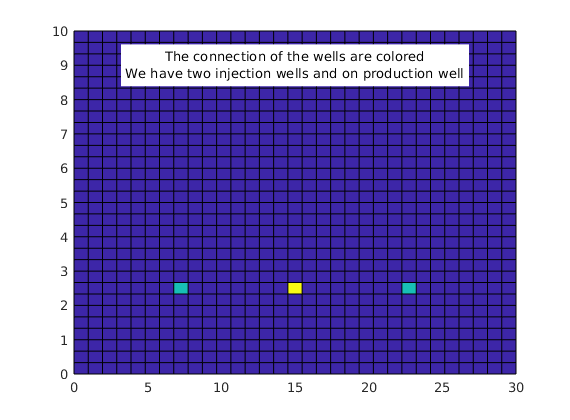
In this example, we demonstrate how one can setup adjoint simulations in a poroelastic simulation in order to compute gradients (or sensitivities) of a given quantity. Here, we will compute the gradient of the vertical displacement (uplift) at a node with respect to the injection rates. We consider a 2D domain, with two injection wells located on the sides and one production well in the middle. The injection rate is given by a schedule (see below). At the production well, we impose a constant pressure. We compute the gradient of the uplift (vertical displacement) at the top of the domain with respect to the injection rates at every time step. We use this gradient information to update the schedule so that the uplift is reduced. Different measures of the time average for the uplift are considered, and they produce different result, see the last plot in this script. Different fluid model can be used (two phases or single phase).

mrstModule add ad-mechanics ad-core ad-props ad-blackoil vemmech deckformat mrst-gui

Setup geometry¶

% We consider a  2D regular cartesian domain

cartDim = [31, 30];
L       = [30, 10];
G = cartGrid(cartDim, L);
G = computeGeometry(G);

Computing normals, areas, and centroids...    Elapsed time is 0.000201 seconds.
Computing cell volumes and centroids...               Elapsed time is 0.001227 seconds.

Setup fluid¶

% We can consider different fluid models

opt.fluid_model = 'single phase';
pRef = 100*barsa;
switch opt.fluid_model
  case 'single phase'
    fluid = initSimpleADIFluid('phases', 'W', 'mu', 1*centi*poise, 'rho', ...
                               1000*kilogram/meter^3, 'c', 1e-4, 'cR', ...
                               4e-10, 'pRef', pRef);
  case 'oil water'
    fluid = initSimpleADIFluid('phases', 'WO', 'mu', [1, 100]*centi*poise, 'n', ...
                               [1, 1], 'rho', [1000, 700]*kilogram/ meter^2, 'c', ...
                               1e-10*[1, 1], 'cR', 1e-10, 'pRef', pRef);
  case 'blackoil'
    error('not yet implemented, but could be easily done!')
  otherwise
    error('fluid_model not recognized.')
end

Setup rock parameters (for flow)¶

rock.perm = darcy*ones(G.cells.num, 1);
rock.poro = 0.3*ones(G.cells.num, 1);

Setup material parameters for Biot and mechanics¶

E          = 1e-2*giga*Pascal; % Young's module
nu         = 0.3;              % Poisson's ratio
alpha      = 1;                % Biot's coefficient
% Convert global properties to cell values
E          = repmat(E, G.cells.num, 1);
nu         = repmat(nu, G.cells.num, 1);
rock.alpha = repmat(alpha, G.cells.num, 1);

Setup boundary conditions for mechanics (no displacement)¶

zero displacement at bottom, left and right sides. We impose a given pressure at the top.

% Gather the Dirichlet boundary faces (zero displacement) at left, bottom and right.
dummyval = 100; % We use pside to recover face at bottom, we use a dummy
                % value for pressure in this function.
bc = pside([], G, 'Xmin', dummyval);
bc = pside(bc, G, 'Xmax', dummyval);
bc = pside(bc, G, 'Ymin', dummyval);
indfacebc = bc.face;

% Get the nodes that belong to the Dirichlet boundary faces.
facetonode = accumarray([G.faces.nodes, rldecode((1 : G.faces.num)', ...
                                                 diff(G.faces.nodePos))], ...
                        ones(numel(G.faces.nodes), 1), [G.nodes.num, ...
                    G.faces.num]);
isbcface = zeros(G.faces.num, 1);
isbcface(indfacebc) = 1;
bcnodes  = find(facetonode*isbcface);
nn       = numel(bcnodes);
u        = zeros(nn, G.griddim);
m        = ones(nn,  G.griddim);
disp_bc  = struct('nodes', bcnodes, 'uu', u, 'mask', m);

% Set a given pressure on the  face at the top.
dummyval = 100; % We use pside to recover face at bottom, we use a dummy
                % value for pressure in this function.
bc = pside([], G, 'Ymax', dummyval);
sidefaces = bc.face;
signcoef = (G.faces.neighbors(sidefaces, 1) == 0) - (G.faces.neighbors(sidefaces, ...
                                                  2) == 0);
n = bsxfun(@times, G.faces.normals(sidefaces, :), signcoef./ ...
           G.faces.areas(sidefaces));
force = bsxfun(@times, n, pRef);
force_bc = struct('faces', sidefaces, 'force', force);

% Construct the boundary conidtion structure for the  mechanical system
el_bc = struct('disp_bc' , disp_bc, 'force_bc', force_bc);

Setup volumetric load for mechanics¶

In this example we do not impose any volumetric force

loadfun = @(x) (0*x);

Gather all the mechanical parameters in a struct¶

mech = struct('E', E, 'nu', nu, 'el_bc', el_bc, 'load', loadfun);

Set gravity off¶

gravity off

Setup model¶

switch opt.fluid_model
  case 'single phase'
    model = MechWaterModel(G, rock, fluid, mech);
  case 'oil water'
    model = MechOilWaterModel(G, rock, fluid, mech);
  case 'blackoil'
    error('not yet implemented')
  otherwise
    error('fluid_model not recognized.')
end

Set up initial reservoir state¶

The initial fluid pressure is set to a constant. We have zero displacement initially.

clear initState;
initState.pressure = pRef*ones(G.cells.num, 1);
switch opt.fluid_model
  case 'single phase'
    init_sat = [1];
  case 'oil water'
    init_sat = [0, 1];
  case 'blackoil'
    error('not yet implemented')
    % init_sat = [0, 1, 0];
    % initState.rs  = 0.5*fluid.rsSat(initState.pressure);
  otherwise
    error('fluid_model not recognized.')
end
% set up initial saturations
initState.s  = ones(G.cells.num, 1)*init_sat;
initState.xd = zeros(nnz(~model.mechModel.operators.isdirdofs), 1);
% We compute the corresponding displacement field using the dedicated
% function computeInitDisp (actually not necessary as the solution should be zero).
initState    = computeInitDisp(model, initState, [], 'pressure', initState.pressure);
initState    = addDerivedQuantities(model.mechModel, initState);

===========================
| It # | disp (disp_dofs) |
===========================
|    1 | 1.17e+09         |
|    2 |*4.06e-07         |
===========================

Setup the wells¶

Two injection wells on the sides and one production well in the middle.

nx = G.cartDims(1);
ny = G.cartDims(2);
switch opt.fluid_model
  case 'single phase'
    comp_inj  = [1];
    comp_prod = [1];
  case 'oil water'
    comp_inj  = [1, 0];
    comp_prod = [0, 1];
  case 'blackoil'
    error('not yet implemented')
  otherwise
    error('fluid_model not recognized.')
end

W = [];
wellopt = {'type', 'rate', 'Sign', 1, 'comp_i', comp_inj};
% Two injection wells vertically aligned, near the bottom
W = addWell(W, G, rock, round(nx/4)   + floor(1/4*ny)*nx, wellopt{:});
W = addWell(W, G, rock, nx + 1 - round(nx/4) + floor(1/4*ny)*nx, wellopt{:});
% production well in the center
wellopt = {'type', 'bhp', 'val', pRef, 'Sign', -1, 'comp_i', comp_prod};
W = addWell(W, G, rock, round(nx/2)   + floor(1/4*ny)*nx, wellopt{:});

% We plot the well location
wellcells = zeros(G.cells.num, 1);
wellcells(W(1).cells) = 1;
wellcells(W(2).cells) = 1;
wellcells(W(3).cells) = 2;
figure
clf
plotCellData(G, wellcells);
comment = ['The connection of the wells are colored' char(10) 'We have two ' ...
          'injection wells and on production well'];
text(0.5, 0.9, comment, 'units', 'normalized', 'horizontalalignment', 'center', ...
     'backgroundcolor', 'white');

% We incorporate the well in a FacilityModel which takes care of coupling all
% the well equations with the reservoir equations

facilityModel = FacilityModel(model.fluidModel);
facilityModel = facilityModel.setupWells(W);
model.FacilityModel = facilityModel;
model = model.validateModel(); % setup consistent fields for model (in
                               % particular the facility model for the fluid
                               % submodel)

Defaulting reference depth to top of formation for well W1. Please specify 'refDepth' optional argument to 'addWell' if you require bhp at a specific depth.
Defaulting reference depth to top of formation for well W2. Please specify 'refDepth' optional argument to 'addWell' if you require bhp at a specific depth.
Defaulting reference depth to top of formation for well W3. Please specify 'refDepth' optional argument to 'addWell' if you require bhp at a specific depth.

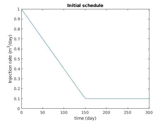
Setup a schedule¶

We set up a schedule where we gradually decrease from a maximum to a minimum injection rate value. Then, we keep the injection rate constant. See plot below.

clear schedule
schedule.step.val     = [1*day*ones(1, 1); 10*day*ones(30, 1)];
nsteps = numel(schedule.step.val);
schedule.step.control = (1 : nsteps)';
valmax = 1*meter^3/day;
valmin = 1e-1*meter^3/day;
ctime = cumsum(schedule.step.val);
flattentime   = 150*day; % Time when we reach the minimal rate value
qW = zeros(nsteps, 1);
for i = 1 : numel(schedule.step.control)
    if ctime(i) < flattentime
        qW(i) = valmin*ctime(i)/flattentime + valmax*(flattentime - ctime(i))/flattentime;
    else
        qW(i) = valmin;
    end
    W(1).val = qW(i);
    W(2).val = qW(i);
    schedule.control(i) = struct('W', W);
end
% We plot the injection schedule
figure
plot(ctime/day, qW*day);
axis([0, ctime(end)/day, 0, 1])
title('Initial schedule');
xlabel('time (day)')
ylabel('Injection rate (m^3/day)');

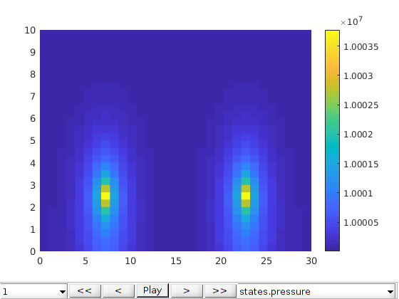
Run the schedule¶

We run the simulation for the given model, initial state and schedule.

[wellSols, states] = simulateScheduleAD(initState, model, schedule);

% We start a visualization tool to inspect the result of the simulation
figure
plotToolbar(G, states);
colorbar

*****************************************************************
********** Starting simulation:    31 steps,   301 days *********
*****************************************************************
Preparing model for simulation...
Model ready for simulation...
Preparing schedule for simulation...
Schedule ready for simulation...
Validating initial state...
...

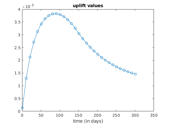
We plot the evolution of the uplift¶

% Get index of a node belonging to the cell at the middle on the top layer.
topcell = floor(nx/2) + nx*(ny - 1);
topface = G.cells.faces(G.cells.facePos(topcell) : (G.cells.facePos(topcell + ...
                                                  1)  - 1), :);
topface = topface(topface(:, 2) == 4, 1);
topnode = G.faces.nodes(G.faces.nodePos(topface)); % takes one node from the
                                                   % top face (the first listed)

laststep = numel(states);
uplift = @(step) (computeUpliftForState(model, states{step}, topnode));
uplifts = arrayfun(uplift, (1 : laststep)');
figure
plot(ctime/day, uplifts, 'o-');
title('uplift values');
xlabel('time (in days)');

Setup of the objective function given by averaged uplift values¶

The adoint framework is general and computes the derivative of a (scalar) objective function of following forms,

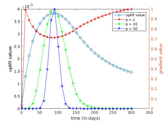
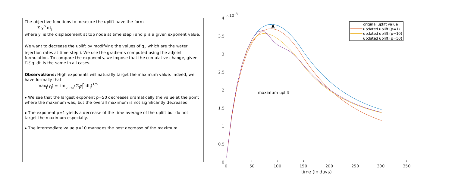
This special form of this objective function allows for a recursive computation of the adjoint variables. We set up our objective function as being a time average of weighted uplift in a node in the middle at the top Given an exponent p, we take

See function objUpliftAver. We consider three values for the exponent p.

Compute gradients using the adjoint formulation for three different exponents¶

np               = 3;
exponents        = cell(np, 1);
adjointGradients = cell(np, 1);

exponents = {1; 10; 50};

for p = 1 : np
    C = 1e3; % For large exponents we need to scale the values to avoid very large
             % or very small objective function
    objUpliftFunc = @(tstep) objUpliftAver(model, states, schedule, topnode, ...
                                           'tStep', tstep, 'computePartials', true, ...
                                           'exponent', exponents{p}, ...
                                           'normalizationConstant', C);
    fprintf('\n***\n*  Start adjoint simulation for exponent p=%g\n*\n', exponents{p});
    adjointGradients{p} = computeGradientAdjointAD(initState, states, model, ...
                                                   schedule, objUpliftFunc);
end

***
*  Start adjoint simulation for exponent p=1
*
Preparing model for simulation...
Model ready for simulation...
Validating initial state...
Initial state ready for simulation.
...

We can check the results from the adjoint computation by using finite difference¶

The function computeGradientAdjointAD sets up this computation check for us. It should be used with a smaller schedule, otherwise the computation is very long.

compute_numerical_derivative = false;
if compute_numerical_derivative
    objUpliftFunc2 = @(wellSols, states, schedule) objUplift(model, states, ...
                                                      schedule, topnode, ...
                                                      'computePartials', ...
                                                      false);
    fdgrad = computeGradientPerturbationAD(initState, model, schedule, ...
                                           objUpliftFunc2, 'perturbation', ...
                                           1e-7);
end

Plots of the results.¶

We plot the uplift values with the gradients (normalized for comparison).

figure
clf
plot(ctime/day, uplifts, 'o-');
ylabel('uplift values');
xlabel('time (in days)');
hold on
yyaxis right

legendtext = {'uplift value'};
set(gca,'ColorOrder',hsv(3));
for p = 1 : np
    grads = cell2mat(adjointGradients{p});
    qWgrad = grads(1, :);
    % we renormalize the gradients to compare the two series of values
    qWgrad = 1/max(qWgrad)*qWgrad;
    plot(ctime/day, qWgrad, '*-');
    legendtext{end + 1} = sprintf('p = %g', exponents{p});
end

ylabel('gradient value')
legend(legendtext);

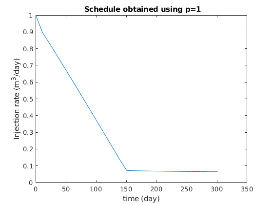
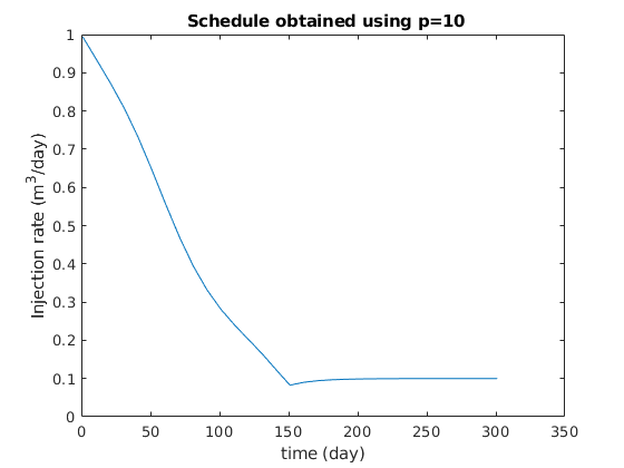
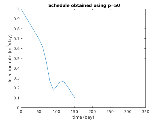
Update of the schedule based on gradient values¶

We use the gradient values computed above to update the schedule so that the uplift, as measured with the three different values of the exponents, is decreased. The absolute minimum uplift is of course zero and it is obtained when we do not inject anything. To avoid this trivial case, we impose the extra requirement that, in all cases, we will have the same decrease in the total injection.

inituplifts = uplifts;
initschedule = schedule;
dts = schedule.step.val;
nsteps = numel(dts);
ctime = cumsum(schedule.step.val);
tottime = ctime(end);

np      = numel(adjointGradients);
uplifts = cell(np, 1);
qWs     = cell(np, 1);

dcqW = 3e-2*meter^3/day*tottime; % this is the total amount of injected fluid we
                                 % are willing to decrease.

for p = 1 : np

    grads = cell2mat(adjointGradients{p});

    qW = zeros(nsteps, 1);
    dqW = cell(2, 1);
    for i = 1 : 2
        dqW{i} = grads(i, :);
        dqW{i} = dcqW/(dqW{i}*dts)*dqW{i};
    end

    schedule = initschedule;
    for i = 1 : numel(schedule.step.control)
        W = schedule.control(i).W;
        % we update the values of the injection rate at each time step using
        % the gradient values.
        W(1).val = W(1).val - dqW{1}(i);
        W(2).val = W(2).val - dqW{2}(i);
        schedule.control(i) = struct('W', W);
        qW(i) = W(1).val;
    end

    qWs{p} = qW;

    figure
    clf
    plot(ctime/day, qW*day);
    title(sprintf(' Schedule obtained using p=%g', exponents{p}));
    xlabel('time (day)');
    ylabel('Injection rate (m^3/day)');

    fprintf('\n***\n*  Start simulation and compute uplift for updated schedule using exponent p=%g\n*\n', exponents{p});
    [wellSols, states] = simulateScheduleAD(initState, model, schedule);

    nsteps = numel(states);
    uplift = @(step) (computeUpliftForState(model, states{step}, topnode));
    uplifts{p} = arrayfun(uplift, (1 : nsteps)');

end

% plot of the results.
figure
set(gcf, 'position', [100, 100, 1500, 600]);
clf
subplot(1, 2, 2)
hold on
plot(ctime/day, inituplifts);
legendtext = {'original uplift value'};
for p = 1 : np
    plot(ctime/day, uplifts{p});
    legendtext{end + 1} = sprintf('updated uplift (p=%g)', exponents{p});
end
xlabel('time (in days)');
legend(legendtext);

% Add some comments to the plot
[y, ind] = max(inituplifts);
x        = ctime(ind)/day;
set(gca, 'position', [0.5, 0.1, 0.4, 0.8], 'units', 'normalized')
xlim     = get(gca, 'xlim');
ylim     = get(gca, 'ylim');
apos  = get(gca, 'position');
xn = apos(1) + (x - xlim(1))/(xlim(2) - xlim(1))*apos(3);
yn = apos(2) + (y - ylim(1))/(ylim(2) - ylim(1))*apos(4);
annotation('textarrow', [xn, xn], [0.5, yn], 'string', 'maximum uplift');

subplot(1, 2, 1)
axis off
comments =  fileread('commentsToPlot.tex');
annotation('textbox', 'units', 'normalized', 'position', [0.05 0.1 0.4 0.8], ...
            'interpreter', 'tex', 'string', comments)

***
*  Start simulation and compute uplift for updated schedule using exponent p=1
*
*****************************************************************
********** Starting simulation:    31 steps,   301 days *********
*****************************************************************
Preparing model for simulation...
...

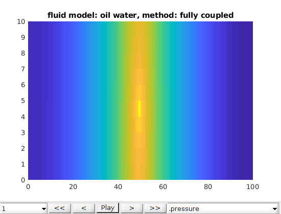
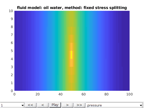
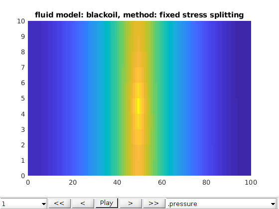
Example of poelasticity simulation on 2D grids¶

Generated from runAll2DCases.m

The implementation of the poroelasticty solver is done in such a way that it is easy to switch between different fluid models and different solving strategy (fully coupled versus splitting). In this example, we run all the combination of these choices for a 2D case. See run2DCase for a presentation of the test case. Options that are run are - fluid model :

solver :

mrstModule add ad-mechanics

clear opt

opt.fluid_model        = 'water';
opt.cartDim            = [100, 10];
opt.L                  = [100, 10];
opt.method             = 'fully coupled';
opt.bc_case            = 'bottom fixed';

opt.nonlinearTolerance = 1e-6;
opt.splittingTolerance = 1e-6;
opt.verbose            = false;
opt.splittingVerbose   = false;

% write intro text for each case
writeIntroText = @(opt)(fprintf('\n*** Start new simulation with\n* fluid model : %s\n* method : %s\n\n', opt.fluid_model, opt.method));

water cases¶

opt.fluid_model = 'water';

opt.method      = 'fully coupled';
writeIntroText(opt);

optvals = cellfun(@(x) opt.(x), fieldnames(opt), 'uniformoutput', false);
optlist = reshape(vertcat(fieldnames(opt)', optvals'), [], 1);
[model, states] = run2DCase(optlist{:});
plot2DPoroExample(model, states, opt);


opt.method      = 'fixed stress splitting';
writeIntroText(opt);
optvals = cellfun(@(x) opt.(x), fieldnames(opt), 'uniformoutput', false);
optlist = reshape(vertcat(fieldnames(opt)', optvals'), [], 1);
[model, states] = run2DCase(optlist{:});
plot2DPoroExample(model, states, opt);

*** Start new simulation with
* fluid model : water
* method : fully coupled

Computing normals, areas, and centroids...    Elapsed time is 0.000176 seconds.
Computing cell volumes and centroids...               Elapsed time is 0.001461 seconds.
Warning: Reference depth for well BHP in well 'inj' is set below well's top-most
...

Two phase oil water phases cases¶

opt.fluid_model = 'oil water';


opt.method      = 'fully coupled';
writeIntroText(opt);
optvals = cellfun(@(x) opt.(x), fieldnames(opt), 'uniformoutput', false);
optlist = reshape(vertcat(fieldnames(opt)', optvals'), [], 1);
[model, states] = run2DCase(optlist{:});
plot2DPoroExample(model, states, opt);


opt.method      = 'fixed stress splitting';
writeIntroText(opt);
optvals = cellfun(@(x) opt.(x), fieldnames(opt), 'uniformoutput', false);
optlist = reshape(vertcat(fieldnames(opt)', optvals'), [], 1);
[model, states] = run2DCase(optlist{:});
plot2DPoroExample(model, states, opt);

*** Start new simulation with
* fluid model : oil water
* method : fully coupled

Computing normals, areas, and centroids...    Elapsed time is 0.000202 seconds.
Computing cell volumes and centroids...               Elapsed time is 0.001247 seconds.
Warning: Reference depth for well BHP in well 'inj' is set below well's top-most
...

Three phases Black-Oil phases cases¶

opt.fluid_model = 'blackoil';


opt.method      = 'fully coupled';
writeIntroText(opt);
optvals = cellfun(@(x) opt.(x), fieldnames(opt), 'uniformoutput', false);
optlist = reshape(vertcat(fieldnames(opt)', optvals'), [], 1);
[model, states] = run2DCase(optlist{:});
plot2DPoroExample(model, states, opt);


opt.method      = 'fixed stress splitting';
writeIntroText(opt);
optvals = cellfun(@(x) opt.(x), fieldnames(opt), 'uniformoutput', false);
optlist = reshape(vertcat(fieldnames(opt)', optvals'), [], 1);
[model, states] = run2DCase(optlist{:});
plot2DPoroExample(model, states, opt);

*** Start new simulation with
* fluid model : blackoil
* method : fully coupled

Computing normals, areas, and centroids...    Elapsed time is 0.000166 seconds.
Computing cell volumes and centroids...               Elapsed time is 0.002171 seconds.
No converter needed in section 'REGIONS'.
...

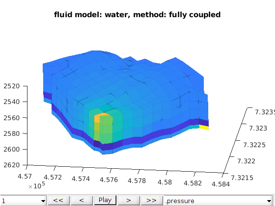
Example: Simulation of poroelasticity on a subset of the Norne case¶

Generated from runAllNorneExamples.m

Same setting as in runAll2Dcases but now for a subset of the Norne case See: runNorneExample and setupNorneExamples

mrstModule add ad-mechanics ad-core ad-props ad-blackoil vemmech deckformat mrst-gui

Summary of the options¶

% opt.norne_case = 'mini Norne'; % 'full' or 'mini Norne'
%
% 'full'       : 7392 cells
% 'mini Norne' :  605 cells
%
% opt.bc_case    = 'bottom fixed'; % 'no displacement' or 'bottom fixed'
%
% 'no displacement' : All nodes belonging to external faces have displacement
%                     equal to zero
% 'bottom fixed'    : The nodes that belong to the bottom have zero
%                     displacement, while a given pressure is imposed on
%                     the external faces that are not bottom faces.
%
% opt.method     = 'fully coupled'; % 'fully coupled' 'fixed stress splitting'
%
% 'fully coupled'          : The mechanical and flow equations are solved fully couplde.
%
% 'fixed stress splitting' : The mechanical and flow equations are solved
%                            sequentially using a fixed stress splitting
%
% opt.fluid_model = 'oil water'; % 'blackoil' 'water' 'oil water'
%
% 'blackoil'     : blackoil model is used for the fluid (gas is injected, see
%                  schedule below)
% 'oil water'    : Two phase oil-water
% 'water' : water model is used for the fluid

clear opt
opt.verbose          = false;
opt.splittingVerbose = false;
opt.norne_case       = 'mini Norne';
opt.bc_case          = 'bottom fixed';

% write intro text for each case
writeIntroText = @(opt)(fprintf('\n*** Start new simulation\n* fluid model : %s\n* method : %s\n\n', opt.fluid_model, opt.method));

water cases¶

opt.fluid_model = 'water';

opt.method = 'fully coupled';
writeIntroText(opt);
optvals = cellfun(@(x) opt.(x), fieldnames(opt), 'uniformoutput', false);
optlist = reshape(vertcat(fieldnames(opt)', optvals'), [], 1);
[model, states] = runNorneExample(optlist{:});
plotNornePoroExample(model, states, opt);

opt.method = 'fixed stress splitting';
writeIntroText(opt);
optvals = cellfun(@(x) opt.(x), fieldnames(opt), 'uniformoutput', false);
optlist = reshape(vertcat(fieldnames(opt)', optvals'), [], 1);
[model, states] = runNorneExample(optlist{:});
plotNornePoroExample(model, states, opt);

*** Start new simulation
* fluid model : water
* method : fully coupled

Reading keyword 'INCLUDE'
 -> '/home/francesca/mrstReleaseCleanRepo/mrst-bitbucket/mrst-core/examples/data/Norne/INCLUDE/IRAP_1005.GRDECL'
Reading keyword 'SPECGRID'
...

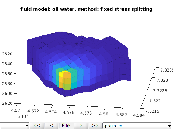
Two phase oil water phases cases¶

opt.fluid_model = 'oil water';

opt.method = 'fully coupled';
writeIntroText(opt);
optvals = cellfun(@(x) opt.(x), fieldnames(opt), 'uniformoutput', false);
optlist = reshape(vertcat(fieldnames(opt)', optvals'), [], 1);
[model, states] = runNorneExample(optlist{:});
plotNornePoroExample(model, states, opt);

opt.method = 'fixed stress splitting';
writeIntroText(opt);
optvals = cellfun(@(x) opt.(x), fieldnames(opt), 'uniformoutput', false);
optlist = reshape(vertcat(fieldnames(opt)', optvals'), [], 1);
[model, states] = runNorneExample(optlist{:});
plotNornePoroExample(model, states, opt);

*** Start new simulation
* fluid model : oil water
* method : fully coupled

Reading keyword 'INCLUDE'
 -> '/home/francesca/mrstReleaseCleanRepo/mrst-bitbucket/mrst-core/examples/data/Norne/INCLUDE/IRAP_1005.GRDECL'
Reading keyword 'SPECGRID'
...

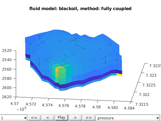
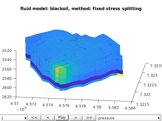
Three phases Black-Oil phases cases¶

opt.fluid_model = 'blackoil';

opt.method = 'fully coupled';
writeIntroText(opt);
optvals = cellfun(@(x) opt.(x), fieldnames(opt), 'uniformoutput', false);
optlist = reshape(vertcat(fieldnames(opt)', optvals'), [], 1);
[model, states] = runNorneExample(optlist{:});
plotNornePoroExample(model, states, opt);

opt.method = 'fixed stress splitting';
writeIntroText(opt);
opt.splittingTolerance = 1e-3;
optvals = cellfun(@(x) opt.(x), fieldnames(opt), 'uniformoutput', false);
optlist = reshape(vertcat(fieldnames(opt)', optvals'), [], 1);
[model, states] = runNorneExample(optlist{:});
plotNornePoroExample(model, states, opt);

*** Start new simulation
* fluid model : blackoil
* method : fully coupled

Reading keyword 'INCLUDE'
 -> '/home/francesca/mrstReleaseCleanRepo/mrst-bitbucket/mrst-core/examples/data/Norne/INCLUDE/IRAP_1005.GRDECL'
Reading keyword 'SPECGRID'
...

function [model, states] = runNorneExample(varargin)

Example: Poroelasticity simulation applied to the Norne case.¶

Generated from runNorneExample.m

The simulation options are gathered in the opt structure. If opt=[] the simulation is run with the default options defined below Summary of the options option ‘norne_case’ :

option ‘bc_case’ :

option ‘method’ :

option ‘fluid_model’ :

%{

Load Norne grid¶

if ~ (makeNorneSubsetAvailable() && makeNorneGRDECL()),
        error('Unable to obtain simulation model subset');
    end


    grdecl = fullfile(getDatasetPath('norne'), 'NORNE.GRDECL');
    grdecl = readGRDECL(grdecl);
    fullCartDims = grdecl.cartDims;
    usys   = getUnitSystem('METRIC');
    grdecl = convertInputUnits(grdecl, usys);
    switch opt.norne_case
      case 'full'
        grdecl = cutGrdecl(grdecl, [10 25; 35 55; 1 22]);
      case 'full padded'
        grdeclo = cutGrdecl(grdecl, [10 25; 35 55; 1 22]);
        oncells = prod(grdeclo.cartDims);
        oindex = 1:oncells;
        oindex = reshape(oindex, grdeclo.cartDims);
        grdecl = padGrdecl(grdeclo, [true, true, true], [[60 50; 40 40] * 10; 10 10], 'relative', true);
        grdecl.ACTNUM = ones(prod(grdecl.cartDims), 1);
        indexmapn = zeros(grdecl.cartDims);
        indexmapn(2:end - 1, 2:end - 1, 2:end - 1) = oindex;
        indexmapn(indexmapn == 0) = prod(grdeclo.cartDims) + 1;
        ocells = indexmapn < prod(grdeclo.cartDims);
        oindex = indexmapn;
      case 'mini Norne'
        grdecl = cutGrdecl(grdecl, [10 20; 35 45; 1 5]);
      otherwise
        error('norne_case not recognized');
    end
    grdecl.ACTNUM = ones(size(grdecl.ACTNUM));
    G = processGRDECL(grdecl);
    G = G(1);
    G = computeGeometry(G);

Reading keyword 'INCLUDE'
 -> '/home/francesca/mrstReleaseCleanRepo/mrst-bitbucket/mrst-core/examples/data/Norne/INCLUDE/IRAP_1005.GRDECL'
Reading keyword 'SPECGRID'
Reading keyword 'COORD'
Reading keyword 'ZCORN'
 <- '/home/francesca/mrstReleaseCleanRepo/mrst-bitbucket/mrst-core/examples/data/Norne/INCLUDE/IRAP_1005.GRDECL'
Reading keyword 'INCLUDE'
 -> '/home/francesca/mrstReleaseCleanRepo/mrst-bitbucket/mrst-core/examples/data/Norne/INCLUDE/ACTNUM_0704.prop'
...

Setup rock parameters (for flow)¶

switch opt.norne_case
      case {'full', 'mini Norne'}
        perm = [grdecl.PERMX, grdecl.PERMY, grdecl.PERMZ];
        rock.perm = perm(G.cells.indexMap, :);
        rock.poro = max(grdecl.PORO(G.cells.indexMap), 0.1);
      case 'full padded'
        perm = [grdeclo.PERMX, grdeclo.PERMY, grdeclo.PERMZ;
                [1 1 1]*milli*darcy ];
        poro = [grdeclo.PORO;0.1];
        rock.perm = perm(oindex(G.cells.indexMap), :);
        rock.poro = max(poro(oindex(G.cells.indexMap)), 0.1);
        [i, j, k] = ind2sub(G.cartDims, G.cells.indexMap);
        ind = (k>1 & k<G.cartDims(3) &  oindex(G.cells.indexMap) == numel(poro));
        rock.perm(ind, :) = rock.perm(ind, :) * 100;
      otherwise
        error('norne_case not recognized');
    end

Setup fluid parameters from SPE1¶

pRef = 270*barsa;
    switch opt.fluid_model
      case 'blackoil'
        pth = getDatasetPath('spe1');
        fn  = fullfile(pth, 'BENCH_SPE1.DATA');
        deck = readEclipseDeck(fn);
        deck = convertDeckUnits(deck);
        fluid = initDeckADIFluid(deck);
        if isfield(fluid, 'pcOW')
            fluid = rmfield(fluid, 'pcOW');
        end
        if isfield(fluid, 'pcOG')
            fluid = rmfield(fluid, 'pcOG');
        end

        % Setup quadratic relative permeabilities, since SPE1 relperm are a bit rough.
        fluid.krW = @(s) s.^2;
        fluid.krG = @(s) s.^2;
        fluid.krOW = @(s) s.^2;
        fluid.krOG = @(s) s.^2;
        pRef = deck.PROPS.PVTW(1);

      case {'oil water'}
        fluid = initSimpleADIFluid('phases', 'WO', 'mu', [1, 10]*centi*poise, ...
                                   'n',  [1, 1], 'rho', [1000, 700]*kilogram/ ...
                                   meter^3, 'c', 1e-10*[1, 1], 'cR', 4e-10, ...
                                   'pRef', pRef);

      case {'water'}
        fluid = initSimpleADIFluid('phases', 'W', 'mu', 1*centi*poise, 'rho', ...
                                   1000*kilogram/meter^3, 'c', 1e-10, ...
                                   'cR', 4e-10, 'pRef', pRef);
      otherwise
        error('fluid_model  not recognized.');
    end

Setup material parameters for Biot and mechanics¶

E          = 1 * giga * Pascal; % Young's module
    nu         = 0.3;               % Poisson's ratio
    alpha      = 1;                 % Biot's coefficient

    % Transform these global properties (uniform) to cell values.
    E          = repmat(E, G.cells.num, 1);
    nu         = repmat(nu, G.cells.num, 1);
    rock.alpha = repmat(alpha, G.cells.num, 1);

Setup boundary conditions for mechanics (no displacement)¶

switch opt.bc_case

      case 'no displacement'

        ind = (G.faces.neighbors(:, 1) == 0 | G.faces.neighbors(:, 2) == 0);
        ind = find(ind);
        nodesind = mcolon(G.faces.nodePos(ind), G.faces.nodePos(ind + 1) - 1);
        nodes = G.faces.nodes(nodesind);
        bcnodes = zeros(G.nodes.num);
        bcnodes(nodes) = 1;
        bcnodes = find(bcnodes == 1);
        nn = numel(bcnodes);
        u = zeros(nn, 3);
        m = ones(nn, 3);
        disp_bc = struct('nodes', bcnodes, 'uu', u, 'mask', m);
        force_bc = [];

      case 'bottom fixed'

        nx = G.cartDims(1);
        ny = G.cartDims(2);
        nz = G.cartDims(3);

        % Find the bottom nodes. On these nodes, we impose zero displacement

        c = zeros(nx*ny*nz, 1);
        c(G.cells.indexMap) = (1 : numel(G.cells.indexMap))';
        bottomcells = c(nx*ny*(nz - 1) +  (1 : (nx*ny))');
        faces = G.cells.faces(mcolon(G.cells.facePos(bottomcells), G.cells.facePos(bottomcells ...
                                                          + 1) - 1), :);
        bottomfaces = faces( faces(:, 2) == 6  , 1);
        indbottom_nodes = mcolon(G.faces.nodePos(bottomfaces), G.faces.nodePos(bottomfaces ...
                                                          + 1) - 1);
        bottom_nodes = G.faces.nodes(indbottom_nodes);
        isbottom_node = false(G.nodes.num, 1);
        isbottom_node(bottom_nodes) = true;
        bcnodes = find(isbottom_node);

        nn = numel(bcnodes);
        u = zeros(nn, 3);
        m = ones(nn, 3);
        disp_bc = struct('nodes', bcnodes, 'uu', u, 'mask', m);

        % Find outer faces that are not at the bottom. On these faces, we impose
        % a given pressure.

        is_outerface1 = (G.faces.neighbors(:, 1) == 0);
        is_outerface1(bottomfaces) = false;
        is_outerface2 = G.faces.neighbors(:, 2) == 0;
        is_outerface2(bottomfaces) = false;

        is_outerface = is_outerface1 | is_outerface2;

        outer_faces = find(is_outerface);

        outer_pressure = pRef;
        signcoef = (G.faces.neighbors(outer_faces, 1) == 0) - ...
            (G.faces.neighbors(outer_faces, 2) == 0);
        n = bsxfun(@times, G.faces.normals(outer_faces, :), signcoef./ ...
                   G.faces.areas(outer_faces));
        force = bsxfun(@times, n, outer_pressure);

        force_bc = struct('faces', outer_faces, 'force', force);


      otherwise
        error('bc_cases not recognized')
    end

    el_bc = struct('disp_bc' , disp_bc, ...
                   'force_bc', force_bc);

Setup load for mechanics¶

% In this example we do not impose any volumetric force
    loadfun = @(x) (0*x);

Gather all the mechanical parameters in a struct¶

mech = struct('E', E, 'nu', nu, 'el_bc', el_bc, 'load', loadfun);

Gravity¶

The gravity in this option affects only the fluid behavior

gravity on;

Setup model¶

modeltype = [opt.method, ' and ', opt.fluid_model];
    fullycoupledOptions = {'verbose', opt.verbose};
    splittingOptions = {'splittingTolerance', opt.splittingTolerance, ...
                        'splittingVerbose', opt.splittingVerbose};
    switch modeltype

      case 'fully coupled and blackoil'
        model = MechBlackOilModel(G, rock, fluid, mech, fullycoupledOptions{: ...
                   });

      case 'fixed stress splitting and blackoil'
        model = MechFluidFixedStressSplitModel(G, rock, fluid, mech, ...
                                               'fluidModelType', 'blackoil', ...
                                               splittingOptions{:});

      case 'fully coupled and oil water'
        model = MechOilWaterModel(G, rock, fluid, mech, fullycoupledOptions{: ...
                   });

      case 'fixed stress splitting and oil water'
        model = MechFluidFixedStressSplitModel(G, rock, fluid, mech, ...
                                               'fluidModelType', 'oil water', ...
                                               splittingOptions{:});

      case 'fully coupled and water'
        model = MechWaterModel(G, rock, fluid, mech, fullycoupledOptions{: });

      case 'fixed stress splitting and water'
        model = MechFluidFixedStressSplitModel(G, rock, fluid, mech, ...
                                               'fluidModelType', 'water', ...
                                               splittingOptions{:});

      otherwise
        error('modeltype not recognized.');
    end

Setup wells¶

W = [];
    refdepth = G.cells.centroids(1, 3); % for example...
    injcell  = 10; % for example...
    prodcell = G.cells.num;

    if strcmp(opt.norne_case, 'full padded')
        injcello = 10; % for example
        pos = [0.457517456153883   7.321672863418036   0.002564025720821] * 1e6;
        [~, injcell] = min(sum(bsxfun(@minus, G.cells.centroids, pos).^2, 2))
        injcell = find(oindex(:) == injcello);
        prodcello = 7392; % for example
        pos = [0.458944373173747   7.322630019653659   0.002783994408426] * 1e6;
        [~, prodcell] = min(sum(bsxfun(@minus, G.cells.centroids, pos).^2, 2));
        prodcell = find(oindex(:) == prodcello);
    end

    W = addWell(W, G, rock, injcell, ...
                'Type'    , 'rate', ...
                'Val'     , 2.5e6/day, ...
                'Sign'    , 1,  ...
                'Comp_i'   , [0, 0, 1], ...
% inject gas
                'Name'    , 'inj',  ...
                'refDepth', refdepth);


    W = addWell(W, G, rock, prodcell, ...
                'Type'    ,'bhp', ...
                'Val'     , pRef, ...
                'Sign'    , -1,  ...
                'Comp_i'   , [0, 1, 0], ...
% one-phase test case
                'Name'    , 'prod',  ...
                'refDepth', refdepth);

    switch opt.fluid_model
      case 'blackoil'
        W(1).compi = [0, 0, 1];
        W(2).compi = [0, 1, 0];
      case 'oil water'
        W(1).compi = [1 0];
        W(1).val   = 1e4/day;
        W(2).compi = [0 1];
      case 'water'
        W(1).compi = [1];
        W(1).val   = 1e4/day;
        W(2).compi = [1];
      otherwise
        error('fluid_model not recognized.')
    end

    facilityModel = FacilityModel(model.fluidModel);
    facilityModel = facilityModel.setupWells(W);
    model.FacilityModel = facilityModel;

Setup schedule¶

schedule.step.val     = [1*day*ones(1, 1); 5*day*ones(20, 1)];
    schedule.step.control = ones(numel(schedule.step.val), 1);
    schedule.control      = struct('W', W);

Setup initial state¶

clear initState;
    initState.pressure = pRef*ones(G.cells.num, 1);
    switch opt.fluid_model
      case 'blackoil'
        init_sat = [0, 1, 0];
        initState.rs  = 0.5*fluid.rsSat(initState.pressure);
      case 'oil water'
        init_sat = [0, 1];
      case 'water'
        init_sat = [1];
      otherwise
        error('fluid_model not recognized.')
    end
    initState.s = ones(G.cells.num, 1)*init_sat;
    initState   = computeInitDisp(model, initState, []);

    [wellSols, states, schedulereport] = simulateScheduleAD(initState, model, schedule);

===========================
| It # | disp (disp_dofs) |
===========================
|    1 | 6.45e+12         |
|    2 | 8.02e-03         |
|    3 |*1.21e-13         |
===========================
*****************************************************************
...

end

ans =

  MechWaterModel with properties:

                mechModel: [1×1 MechanicMechModel]
          MechPrimaryVars: []
                  mechfds: {'xd'  'uu'  'u'  'stress'  'strain'  'vdiv'}
...

ad-mechanics: Coupled flow and mechanics¶

Examples¶

2D example for poroelasticity¶

Load required modules¶

Setup default options¶

Setup grid¶

Setup rock parameters (for flow)¶

Setup fluid parameters from SPE1¶

Setup material parameters for Biot and mechanics¶

Setup boundary conditions for mechanics (no displacement)¶

Setup load for mechanics¶

Gather all the mechanical parameters in a struct¶

Gravity¶

Setup model¶

Setup wells¶

Setup schedule¶

Setup initial state¶

Computation of Gradients using Adjoint simulations¶

Setup geometry¶

Setup fluid¶

Setup rock parameters (for flow)¶

Setup material parameters for Biot and mechanics¶

Setup boundary conditions for mechanics (no displacement)¶

Setup volumetric load for mechanics¶

Gather all the mechanical parameters in a struct¶

Set gravity off¶

Setup model¶

Set up initial reservoir state¶

Setup the wells¶

Setup a schedule¶

Run the schedule¶

We plot the evolution of the uplift¶

Setup of the objective function given by averaged uplift values¶

Compute gradients using the adjoint formulation for three different exponents¶

We can check the results from the adjoint computation by using finite difference¶

Plots of the results.¶

Update of the schedule based on gradient values¶

Example of poelasticity simulation on 2D grids¶

water cases¶

Two phase oil water phases cases¶

Three phases Black-Oil phases cases¶

Example: Simulation of poroelasticity on a subset of the Norne case¶

Summary of the options¶

water cases¶

Two phase oil water phases cases¶

Three phases Black-Oil phases cases¶

Example: Poroelasticity simulation applied to the Norne case.¶

Load Norne grid¶

Setup rock parameters (for flow)¶

Setup fluid parameters from SPE1¶

Setup material parameters for Biot and mechanics¶

Setup boundary conditions for mechanics (no displacement)¶

Setup load for mechanics¶

Gather all the mechanical parameters in a struct¶

Gravity¶

Setup model¶

Setup wells¶

Setup schedule¶

Setup initial state¶

`ad-mechanics`: Coupled flow and mechanics¶