adjoint: Two-phase, incompressible adjoint solvers
Implements strategies for production optimisation based on adjoint formulations. This enables for, instance, optimization of net present value constrained by the bottom-hole pressure in wells. This module is limited to two-phase, incompressible flow as implemented in the incomp module. For optimization problems with more complex fluid physics, the newer “optimization” module is recommended.
Utilities
-
Contents¶ ADJOINT Add-on module for adjoint-based production optimisation
- Files
- addAdjointWellFields - SYNOPSIS: adjointFluidFields - Extend fluid functionality with fields needed in (2nd order) adjoint imp. assembleWellSystem - Generate pressure linear system components for wells. computeAdjointRHS - Compute adjoint ‘pressure’ rhs computeGradient - compute gradient for control variables and project according to computeNumericalGradient - compute numerical gradient controls2RHS - Create mappings A_N, b_N, A_D, b_D such that controls2Wells - Create mappings A_N, b_N, A_D, b_D such that generateUpstreamTransportMatrix - generateUpstreamTransportMatrix for use in saturation solver initControls - initControls – Initialize control structure based on well schedule initSchedule - initSchedule – Initialize schedule structure based on well W. optimizeObjective - optimizeObjective – Run whole optimization proccess using ad-hoc line projectGradient - Project gradient according to linear input constraints. Handles box-constraints and runAdjoint - runAdjoint – Run adjoint simulation based on simRes and schedule. runSchedule - runSchedule – Run simulation based on schedule. solveAdjointPressureSystem - Find current time step (search for empty slots in adjRes) solveAdjointTransportSystem - Find current time step (search for empty slots in adjRes) updateSchedule - Update schedule based on controls updateWells - Update wells based on schedule time step dispControls - Display control values. dispSchedule - Display schedule values lineSearchAgr - Run agressive line search based on given gradient. solveIncompFlowLocal - Local version of solveIncompFlow for use with adjoint module. Local
-
addAdjointWellFields(CG, W, varargin)¶ Synopsis:
W = addAdjointWellFields(CG, W, varargin)
W = addAdjointWellFields(CG, W, 'OverlapWell', 0, 'OverlapBlock', 4);
Description:
Hack for the adjoint code: Add additional fields to the Well-structure. The added fields are coarseCells and optionally CS.overlap and CS.wellOverlap.
Needed in updateWells and createSingleCellPseudoWells.
-
adjointFluidFields(fluid)¶ Extend fluid functionality with fields needed in (2nd order) adjoint imp.
Synopsis:
fluid = adjointFluidFields(fluid)
Parameters: fluid – A ‘fluid_structure’. Returns: fluid – Updated fluid structure now containing additional fields - dLtInv (state) – d/ds (1 / lambda_t(state)) - d2LtInv(state) – d^2/ds^2 (1 / lambda_t(state)) - d2fw (state) – d^2/ds^2 f_w(state) See also
fluid_structure.
-
assembleWellSystem(G, W, varargin)¶ Generate pressure linear system components for wells.
Synopsis:
W = assembleWellSystem(G, W)
W = assembleWellSystem(G, W, 'pn1', pv1, ...)
Parameters: - G – Grid structure as described by grid_structure.
- W – Well structure as defined by addWell &c.
- 'pn'/pv –
List of ‘key’/value pairs defining optional parameters. The supported options are:
- Type – The kind of system to assemble. The choice made
- for this option influences which pressure solvers can be employed later. String. Default value = ‘hybrid’.
- Supported values are:
- ’hybrid’ : Hybrid system with inverse mass matrix
- (BI) for Schur complement reduction.
- ’mixed’ : Hybrid system with regular mass matrix (B)
- for reduction to mixed form.
Note: The value of this option should match the option pair passed to function computeMimeticIP.
Returns: W – Updated well structure. Function assembleWellSystem adds field ‘S’ to each well in ‘W’. The well system W(k).S has the following fields:
S.BI/S.B – Well hybrid system (inverse) ‘mass’ matrix. S.C – Well hybrid system discrete divergence operator. S.D – Well hybrid system flux continuity matrix. S.RHS – Well hybrid linear system right hand side.
See also
-
computeAdjointRHS(G, W, f_res)¶ Compute adjoint ‘pressure’ rhs for use in e.g. function solveAdjointPressureSystem
Synopsis:
b = computeAdjoint(G, W, f_res, f_w)
DESCRIPTION: Computes adjoint ‘pressure’ rhs as input to solveIncompFlow in function solveAdjointPressureSystem
Parameters: - G – Grid data structure.
- W – Well structure as defined by addWell &c.
- f_res – Adjoint reservoir ‘pressure’ condtions
Returns: b – Ajoint pressure rhs to be passed directly as option ‘rhs’ to solveIncompFlow.
-
computeGradient(W, adjRes, schedule, controls)¶ compute gradient for control variables and project according to linEqConst A*u = b => A*grad = 0 Thus the projected gradient is
grad_p = (I - A’*inv(A*A’)*A)*grad
-
computeNumericalGradient(simRes, G, S, W, rock, fluid, schedule, controls, objectiveFunction)¶ compute numerical gradient
-
controls2RHS(W, schedule, controls)¶ - Create mappings A_N, b_N, A_D, b_D such that
- q_{tot,N}^n = A_N{n}*u^n + b_N{n} p_{w,D}^n = A_D{n}*u^n + b_D{n}
where u^n is the set of controll variables at step n
-
controls2Wells(W, schedule, controls)¶ - Create mappings A_N, b_N, A_D, b_D such that
- q_{tot,N}^n = A_N{n}*u^n + b_N{n} p_{w,D}^n = A_D{n}*u^n + b_D{n}
where u^n is the set of controll variables at step n
-
dispControls(controls, schedule, varargin)¶ Display control values.
-
dispSchedule(schedule, varargin)¶ Display schedule values
-
generateUpstreamTransportMatrix(G, S, W, resSol, wellSol, varargin)¶ generateUpstreamTransportMatrix for use in saturation solver
SYNOPSIS: [A, qPluss, signQ] = generateUpstreamTransportMatrix(G, S, W, resSol, …
wellSol, pn1, pv1, …)Description:
Generates sparse matrix A(cellFlux) which is used in transport solver s1 = s0 + dt*Dv*(Af(s) + q+). Assumes no-flow boundary conditions on all cell-faces
signQ is useful for differentation of max(q, 0)/min(q, 0) wrt to q, when q is zero
REQUIRED PARAMETERS:
Keyword Arguments: - Transpose – if true, the transpose of a is given (default false)
- VectorOutput – if true, output A is a struct with fields ‘i’, ‘j’ and ‘qMinus’, such that A = sparse(i, j, -cellFlux) + diag(qMinus) (NOTE MINUSES). Default value is false
- RelativeThreshold – Considers values below max(abs(cellflux))*RealtiveThreshold as zero (default 0)
-
initControls(schedule, varargin)¶ initControls – Initialize control structure based on well schedule
Synopsis:
controls = initControls(schedule, 'pn', pv, ...)
Description:
Initialize controls
Parameters: - schedule – schedule structure
- 'pn'/pv –
List of ‘key’/value pairs defining optional parameters. The supported options are:
- ControllableWells : indices to wells which will be
- controlled (default all)
- BHPMaxMin : max/min value for bhp-wells,(default [-Inf Inf])
- RateMaxMin : max/min value for rate-wells,(default [-Inf Inf])
- MaxMin : matrix of size numControls x 2,
- where each row contains the max and min value for the corresponding control. Aternative to the two above
- NumControlSteps : number of control steps (default number of time steps)
- LinEqConst : linear equality constraints of the
- form Au = b given in the form {A_1, b_1, A_2, b_2, …}
- Verbose : Display Control vars using dispControls
Returns: controls – Initialized control structure having fields - well : #controllable wells x 1 structure having
fields:
- wellNum : index to current well in schedule (and W)
- values : values for each timeStep
- bhpMaxMin :
- rateMAxMin :
- linEqConst : linear equality contraints structure having fields:
- A
- b
See also
-
initSchedule(W, varargin)¶ initSchedule – Initialize schedule structure based on well W.
Synopsis:
shedule = initSchedule(W, 'pn', pv, ...)
Description:
Initialize schedule
Parameters: - W – well structure
- 'pn'/pv –
List of ‘key’/value pairs defining optional parameters. The supported options are:
- NumSteps : number of simulation time steps (default 1)
- TotalTime : total simualtion time (default 1)
- TimeSteps : endtime for each time step assuming t_0 = 0 (alterative to two previous pns)
- Verbose : display schedule with dispSchedule
Returns: schedule – Initialized numSteps x 1 rate schedule structure having fields - timeInterval – [startTime endTime] - names – {name_1, …, name_n} - types – {welltype_1, … , welltype_n} - values – {val_1, …, val_2}
See also
-
lineSearchAgr(simRes, G, S, W, rock, fluid, schedule, controls, grad, objectiveFunction, stepSize, figProps, opt)¶ Run agressive line search based on given gradient. Handles box-constraints and linear equality - and (probably not) inequality-constaints based on iteratively applying the constrints to the gradient until convergence.
Synopsis:
[simRes, schedule, controls, data] = lineSearch(...
  simRes, G, S, W, rock, fluid, schedule, controls, grad, objectiveFunction, ...
  stepSize, figProps, opt)
- DISCRIPTION:
Project gradient according to constraints iteratively until tollerance ConstTol is met or max number of iterations MaxConstIts is met (returnes failure). Constraints are applied in the following order:
- Box const.
- Lin. UnEq. const.
- Lin. Eq. const.
The resulting norm of the projected gradient is used as stopping criteria
- Line search along projected gradient:
Uses three points [x1 x2 x3] = [0 .5 1]*stepSize (a) If projected gradient pgrad(x2)=pgrad(x3), then on boundary,
done
- If obj(x1)<obj(x2)<obj(x3), set stepSize=2*stepSize goto (a)
- If obj(x1)>obj(x2), set stepSize = .5*stepSize goto (a)
- Find max on quad-curve through (x1, x2, x3) done
Parameters: - S, W, rock, fluid (G,) – usual structures
- simRes –
…
- controls (schedule,) –
…
- grad – gradien as given by computeGradient
- objectiveFunction – handle to objective function
- 'pn'/pv –
- List of ‘key’/value pairs defining optional parameters. The
- supported options are:
- MaxPoints : maximum number of points before to
- terminate line search algorithm
- LinSrchTol : line search relative tolerance
- StepSize : Step size
- ConstTol : Relative contraint satisfaction tol
- MaxConstIts : max number of its for constraint satisfaction
- VerboseLevel : amount of output to screen
Returns: simRes – Results for ‘best’ forward simulation
schedule
controls
data – structure with fields value : objective function value for best run relNormGrad : relative norm of gradient |du|/|objective| success : whether or line search procedure succeeded fraction : optimal fraction obtained during the line
search
SEE ALSO:
-
optimizeObjective(G, S, W, rock, fluid, resSolInit, schedule, controls, objectiveFunction, varargin)¶ optimizeObjective – Run whole optimization proccess using ad-hoc line search. A linkage with an external optimizer or use of matlabs optimizer toolbox (e.g., fmincon)is recommended.
Synopsis:
[simRes, schedule, controls, output] = optimizeObjective( ...
                     G, S, W, rock, fluid, resSolInit, ...
                     schedule, controls, objectiveFunction, varargin)
Parameters: - S, W, rock, fluid (G,) – usual structures
- resSolInit – initial ‘solution’ minimum containing field resSol.sw
- controls (schedule,) –
…
- objectiveFunction – handle to objective function
- 'pn'/pv – List of ‘key’/value pairs defining optional parameters. The supported options are:
:param : gradTol : stopping criterion for scaled gradien :param : objChangeTol : stopping criterion for realitive change in objective
function:param : stepSize : initial step size :param : VerboseLevel : level of output to screen during progress (default: 0).
- < 0 : no output
- 0 : minumal 1 : quite a bit 2 : loads
- :param : PlotProgress : whether or not to plot output during progress
- (default: true)
- :param : OutputLevel : level of output given in structure output (default: 0)
- < 0 = nothing (empty)
- 0 = objective function value for every
- iteration
1 = ?
Returns: - simRes – Results for last (optimal) simulation
- schedule
- controls
- outPut – as described above
SEE ALSO:
-
projectGradient(controls, du, varargin)¶ Project gradient according to linear input constraints. Handles box-constraints and linear equality - and inequality-constraints based on iteratively applying the constraints to the gradient until convergence.
Synopsis:
[pGrad] = projectGradient(...
  simRes, G, S, W, rock, fluid, schedule, controls, grad, objectiveFunction, varargin)
- DISCRIPTION:
Project gradient according to constraints iteratively until tollerance ConstTol is met or max number of iterations MaxConstIts is met (returnes failure). Constraints are applied in the following order:
- Box const.
- Lin. InEq. const.
- Lin. Eq. const.
Parameters: - grad (controls,) –
- 'pn'/pv –
- List of ‘key’/value pairs defining optional parameters. The
- supported options are:
- ConstTol : Relative contraint satisfaction tol
- MaxConstIts : max number of its for constraint satisfaction
- VerboseLevel : amount of output to screen
Returns: pGrad – projected gradient
SEE ALSO:
-
runAdjoint(simRes, G, S, W, rock, fluid, schedule, controls, objectiveFunction, varargin)¶ runAdjoint – Run adjoint simulation based on simRes and schedule.
Synopsis:
adjRes = runAdjoint(simRes, G, S, W, fluid, schedule, objective, pn, pv, ...)
DESCRIPTION:
Parameters: - simRes –
- G – Grid data structure.
- S –
- W –
- fluid –
- schedule –
- objective – function handle
Returns: adjRes – numSteps x 1 structure having fields - timeInterval - resSol - wellSol
SEE ALSO:
-
runSchedule(resSolInit, G, S, W, rock, fluid, schedule, varargin)¶ runSchedule – Run simulation based on schedule.
Synopsis:
simRes = runSchedule(resSolInit, G, S, W, fluid, schedule, pn, pv, ...)
DESCRIPTION:
Parameters: - resSolInit –
- G – Grid data structure.
- S –
- W –
- fluid –
- schedule –
Returns: simRes – (numSteps+1) x 1 structure having fields - timeInterval - resSol - wellSol
SEE ALSO:
-
solveAdjointPressureSystem(G, S, W, rock, fluid, simRes, adjRes, obj, varargin)¶ Find current time step (search for empty slots in adjRes) NOTE: actually curent time step +1
-
solveAdjointTransportSystem(G, S, W, rock, fluid, simRes, adjRes, obj, varargin)¶ Find current time step (search for empty slots in adjRes) NOTE: actually curent time step +1
-
solveIncompFlowLocal(state, g, s, fluid, varargin)¶ Local version of solveIncompFlow for use with adjoint module. Local version has the additional option to supply right-hand-side to system directly. In addition, there is som extra slack in the assertion statement that checks sum(rates)=0 when only rate-controlled wells are present. This to prevent crash if input-constraint handling is not set to machine precision.
Synopsis:
state = solveIncompFlow(state, G, S, fluid)
state = solveIncompFlow(state, G, S, fluid, 'pn1', pv1, ...)
Description:
This function assembles and solves a (block) system of linear equations defining interface fluxes and cell and interface pressures at the next time step in a sequential splitting scheme for the reservoir simulation problem defined by Darcy’s law and a given set of external influences (wells, sources, and boundary conditions).
Parameters: - state – Reservoir and well solution structure either properly initialized from function ‘initState’, or the results from a previous call to function ‘solveIncompFlow’ and, possibly, a transport solver such as function ‘explicitTransport’.
- S (G,) – Grid and (mimetic) linear system data structures as defined by function ‘computeMimeticIP’.
- fluid – Fluid data structure as described by ‘fluid_structure’.
Keyword Arguments: wells – Well structure as defined by function ‘addWell’. May be empty (i.e., W = []) which is interpreted as a model without any wells.
bc – Boundary condition structure as defined by function ‘addBC’. This structure accounts for all external boundary conditions to the reservoir flow. May be empty (i.e., bc = []) which is interpreted as all external no-flow (homogeneous Neumann) conditions.
src – Explicit source contributions as defined by function ‘addSource’. May be empty (i.e., src = []) which is interpreted as a reservoir model without explicit sources.
rhs – Supply system right-hand side ‘b’ directly. Overrides internally constructed system right-hand side. Must be a three-element cell array, the elements of which are correctly sized for the block system component to be replaced.
NOTE: This is a special purpose option for use by code which needs to modify the system of linear equations directly, e.g., the ‘adjoint’ code.
Solver – Which solver mode function ‘solveIncompFlow’ should employ in assembling and solving the block system of linear equations. String. Default value: Solver = ‘hybrid’.
- Supported values are:
- ‘hybrid’ –
Assemble and solve hybrid system for interface pressures. System is eventually solved by Schur complement reduction and back substitution.
The system ‘S’ must in this case be assembled by passing option pair (‘Type’,’hybrid’) or option pair (‘Type’,’comp_hybrid’) to function ‘computeMimeticIP’.
- ‘mixed’ –
Assemble and solve a hybrid system for interface pressures, cell pressures and interface fluxes. System is eventually reduced to a mixed system as per function ‘mixedSymm’.
The system ‘S’ must in this case be assembled by passing option pair (‘Type’,’mixed’) or option pair (‘Type’,’comp_hybrid’) to function ‘computeMimeticIP’.
- ‘tpfa’ –
Assemble and solve a cell-centred system for cell pressures. Interface fluxes recovered through back substitution.
The system ‘S’ must in this case be assembled by passing option pair (‘Type’,’mixed’) or option pair (‘Type’,’comp_hybrid’) to function ‘computeMimeticIP’.
LinSolve – Handle to linear system solver software to which the fully assembled system of linear equations will be passed. Assumed to support the syntax
x = LinSolve(A, b)
in order to solve a system Ax=b of linear equations. Default value: LinSolve = @mldivide (backslash).
MatrixOutput – Whether or not to return the final system matrix ‘A’ to the caller of function ‘solveIncompFlow’. Logical. Default value: MatrixOutput = FALSE.
Returns: state – Update reservoir and well solution structure with new values for the fields:
- pressure – Pressure values for all cells in the
discretised reservoir model, ‘G’.
- facePressure –
Pressure values for all interfaces in the discretised reservoir model, ‘G’.
- flux – Flux across global interfaces corresponding to
the rows of ‘G.faces.neighbors’.
- A – System matrix. Only returned if specifically
requested by setting option ‘MatrixOutput’.
- wellSol – Well solution structure array, one element for
each well in the model, with new values for the fields:
- flux – Perforation fluxes through all
- perforations for corresponding well. The fluxes are interpreted as injection fluxes, meaning positive values correspond to injection into reservoir while negative values mean production/extraction out of reservoir.
- pressure – Well bottom-hole pressure.
Note
If there are no external influences, i.e., if all of the structures ‘W’, ‘bc’, and ‘src’ are empty and there are no effects of gravity, and no system right hand side has been supplied externally, then the input values ‘xr’ and ‘xw’ are returned unchanged and a warning is printed in the command window. This warning is printed with message ID
‘solveIncompFlow:DrivingForce:Missing’See also
computeMimeticIP,addBC,addSource,addWell,initSimpleFluidinitState,solveIncompFlowMS.
-
updateSchedule(controls, schedule)¶ Update schedule based on controls
-
updateWells(W, scheduleStep)¶ Update wells based on schedule time step
-
Contents¶ Files recovery - Objective function calculating water volume at last time step simpleNPV - Simple net-present-value function - no discount factor
-
recovery(G, S, W, rock, fluid, simRes, schedule, controls, varargin)¶ Objective function calculating water volume at last time step
Synopsis:
obj = (G, S, W, rock, fluid, simRes, schedule, controls, varargin)
Description:
Computes value of objective function for given simulation, and partial derivatives of variables if varargin > 6
Parameters: simRes – Returns: obj – structure with fields val - value of objective function SEE ALSO:
-
simpleNPV(G, S, W, rock, fluid, simRes, schedule, controls, varargin)¶ Simple net-present-value function - no discount factor
Synopsis:
obj = simpleNPV(G, S, W, rock, fluid, simRes, schedule, controls)
Description:
Computes value of objective function for given simulation, and partial derivatives of variables if varargin > 6
Parameters: simRes – Returns: obj – structure with fields SEE ALSO:
Examples
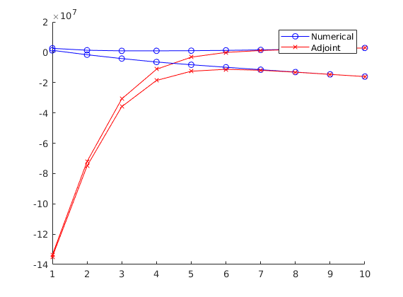
Compare Gradient Computed Numerically and by Adjoint Equations
Generated from compareGradients.m
mrstModule add adjoint mimetic incomp
Setup model
verbose = true;
verboseLevel = 1;

nx = 10; ny = 10; nz = 1;
G  = cartGrid([nx ny nz]);
G  = computeGeometry(G);

rock.perm = exp(( 3*rand(nx*ny, 1) + 1))*100*milli*darcy;
rock.perm = ones( size(rock.perm) )*milli*darcy;
rock.poro = repmat(0.3, [G.cells.num, 1]);

fluid  = initCoreyFluid('mu' , [   1,   5].*centi*poise    , ...
                        'rho', [1014, 859]*kilogram/meter^3, ...
                        'n'  , [   2,   2]                 , ...
                        'sr' , [   0,   0]                 , ...
                        'kwm', [   1,   1]);

fluid  = adjointFluidFields(fluid);

S = computeMimeticIP(G, rock, 'Type', 'comp_hybrid', 'Verbose', verbose);
Processing Cells   1 : 100 of 100 ... done (0.00 [s], 5.02e+04 cells/second)
Total 3D Geometry Processing Time = 0.002 [s]
Using inner product: 'ip_simple'.
Computing cell inner products ...             Elapsed time is 0.028347 seconds.
Assembling global inner product matrix ...    Elapsed time is 0.000327 seconds.
Max error in inverse = 2.9976e-15
Choose objective function
objectiveFunction = str2func('simpleNPV');
%objectiveFunction = str2func('recovery');
Introduce wells
radius = .1;
W = addWell([], G, rock, 1         , 'Type', 'bhp' , 'Val',  100*barsa, 'Radius', radius, 'Name', 'i1', 'Comp_i', [1, 0], 'InnerProduct', 'ip_tpf');
W = addWell( W, G, rock, nx        , 'Type', 'rate', 'Val',  -.5/day  , 'Radius', radius, 'Name', 'p1', 'Comp_i', [0, 1], 'InnerProduct', 'ip_tpf');
W = addWell( W, G, rock, nx*ny-nx+1, 'Type', 'rate', 'Val',  -.5/day  , 'Radius', radius, 'Name', 'p3', 'Comp_i', [0, 1], 'InnerProduct', 'ip_tpf');
W = addWell( W, G, rock, nx*ny     , 'Type', 'rate', 'Val',  -.5/day  , 'Radius', radius, 'Name', 'p3', 'Comp_i', [0, 1], 'InnerProduct', 'ip_tpf');

W = assembleWellSystem(G, W, 'Type', 'comp_hybrid');

resSolInit = initResSol(G, 0.0);
resSolInit.wellSol = initWellSol(W, 0);


totVol   = sum(G.cells.volumes.*rock.poro);
schedule = initSchedule(W, 'NumSteps', 10, 'TotalTime', totVol*day, 'Verbose', verbose);


controls = initControls(schedule, 'ControllableWells', (2:4), ...
                                  'Verbose', verbose, ...
                                  'NumControlSteps', 10);
Defaulting reference depth to top of formation for well i1. Please specify 'refDepth' optional argument to 'addWell' if you require bhp at a specific depth.
Defaulting reference depth to top of formation for well p1. Please specify 'refDepth' optional argument to 'addWell' if you require bhp at a specific depth.
Defaulting reference depth to top of formation for well p3. Please specify 'refDepth' optional argument to 'addWell' if you require bhp at a specific depth.
Defaulting reference depth to top of formation for well p3. Please specify 'refDepth' optional argument to 'addWell' if you require bhp at a specific depth.

----------------- DISPLAYING SCHEDULE ----------------

Time interval :  0.00 - 259200.00
...
Forward run
simRes = runSchedule(resSolInit, G, S, W, rock, fluid, schedule, ...
                             'VerboseLevel', verboseLevel);
----------------- DISPLAYING SCHEDULE ----------------

Time interval :  0.00 - 259200.00
Well name           Type          Value
       i1            bhp       10000000
       p1           rate     -5.787e-06
       p3           rate     -5.787e-06
...
Adjoint run
adjRes = runAdjoint(simRes, G, S, W, rock, fluid, schedule, controls, ...
                    objectiveFunction, 'VerboseLevel', verboseLevel);
grad   = computeGradient(W, adjRes, schedule, controls);

numGrad = computeNumericalGradient(simRes, G, S, W, rock, fluid, ...
                                   schedule, controls, objectiveFunction)
adjGrad = cell2mat(grad)
******* Starting adjoint simulation *******
Time step  10 of  10,   Transport:    0.017 sec,   Pressure:    0.024 sec
Time step   9 of  10,   Transport:    0.006 sec,   Pressure:    0.012 sec
Time step   8 of  10,   Transport:    0.011 sec,   Pressure:    0.007 sec
Time step   7 of  10,   Transport:    0.002 sec,   Pressure:    0.006 sec
Time step   6 of  10,   Transport:    0.010 sec,   Pressure:    0.023 sec
Time step   5 of  10,   Transport:    0.007 sec,   Pressure:    0.006 sec
...
Plot results
igure; hold on
for k = 1 : size(numGrad, 1);
    plot(numGrad(k,:), '-ob');
    plot(adjGrad(k,:), '-xr');
end
legend('Numerical', 'Adjoint')
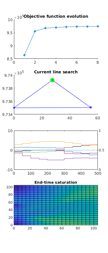
Simple Adjoint Test Using BHP-control
Generated from simpleBHPOpt.m
mrstModule add adjoint mimetic incomp

% whether or not to show output
verbose = false;
verboseLevel = 0;
Define model
nx = 21; ny = 21; nz = 1;
G = cartGrid([nx ny nz], [5*nx 5*ny 1*nz]);
G = computeGeometry(G);

c = G.cells.centroids;
rock.perm  = max(10*sin(c(:,2)/25+.5*cos(c(:,1)/25))-9, .01)*1000*milli*darcy;
rock.poro  = repmat(0.3, [G.cells.num, 1]);

fluid  = initCoreyFluid('mu' , [1, 5] .* centi*poise, ...
                        'rho', [1014, 859].*kilogram/meter^3, ...
                        'n'  , [2, 2], 'sr', [0, 0], 'kwm', [1, 1]);
fluid  = adjointFluidFields(fluid);
Processing Cells   1 : 441 of 441 ... done (0.01 [s], 7.67e+04 cells/second)
Total 3D Geometry Processing Time = 0.006 [s]
Wells and initial rates
radius = .1;
totVol = sum(poreVolume(G, rock));
totTime = 500*day;
W = [];
% Injectors along left side:
nInj = 3; % > 1
pos  = (1 : (ny-1)/(nInj-1) : ny)';
posInj  = round(pos);
for k = 1:nInj
    nm = ['inj', num2str(k)];
    W = addWell(W, G, rock, 1+(posInj(k)-1)*nx, 'Type', 'bhp' , 'Val', 500*barsa, ...
                'Radius', radius, 'Name', nm, 'Comp_i', [1, 0], 'Sign', 1, 'InnerProduct', 'ip_tpf');
end
% Producers along right side:
nProd = 5; % >1
pos  = (1 : (ny-1)/(nProd-1) : ny)';
posProd  = round(pos);
for k = 1:nProd
    nm = ['prod', num2str(k)];
    W = addWell(W, G, rock, nx+(posProd(k)-1)*nx, 'Type', 'bhp' , 'Val', 150*barsa, ...
                'Radius', radius, 'Name', nm, 'Comp_i', [1, 0], 'Sign', -1, 'InnerProduct', 'ip_tpf');
end
Defaulting reference depth to top of formation for well inj1. Please specify 'refDepth' optional argument to 'addWell' if you require bhp at a specific depth.
Defaulting reference depth to top of formation for well inj2. Please specify 'refDepth' optional argument to 'addWell' if you require bhp at a specific depth.
Defaulting reference depth to top of formation for well inj3. Please specify 'refDepth' optional argument to 'addWell' if you require bhp at a specific depth.
Defaulting reference depth to top of formation for well prod1. Please specify 'refDepth' optional argument to 'addWell' if you require bhp at a specific depth.
Defaulting reference depth to top of formation for well prod2. Please specify 'refDepth' optional argument to 'addWell' if you require bhp at a specific depth.
Defaulting reference depth to top of formation for well prod3. Please specify 'refDepth' optional argument to 'addWell' if you require bhp at a specific depth.
Defaulting reference depth to top of formation for well prod4. Please specify 'refDepth' optional argument to 'addWell' if you require bhp at a specific depth.
Defaulting reference depth to top of formation for well prod5. Please specify 'refDepth' optional argument to 'addWell' if you require bhp at a specific depth.
System components
S = computeMimeticIP(G, rock, 'Type', 'comp_hybrid', 'Verbose', verbose, ...
                     'InnerProduct', 'ip_tpf');
W = assembleWellSystem(G, W, 'Type', 'comp_hybrid');
Initialize
state = initResSol(G, 0.0);
state.wellSol = initWellSol(W, 0);
Objective function
objectiveFunction = str2func('simpleNPV');
Initialize schedule and controls
numSteps = 10;
schedule = initSchedule(W, 'NumSteps', numSteps, 'TotalTime', ...
                        totTime, 'Verbose', verbose);

% box constraints for each well [min rate, max rate]
box = [repmat([300*barsa 700*barsa], nInj, 1); repmat([100*barsa 200*barsa], nProd, 1)];
controls = initControls(schedule, 'ControllableWells', (1:numel(W)), ...
                                  'MinMax', box, ...
                                  'Verbose', verbose, ...
                                  'NumControlSteps', numSteps);
Run optimization
simRes, schedule, controls, out] = optimizeObjective(G, S, W, rock, ...
                                        fluid, state, schedule, ...
                                        controls, objectiveFunction, ...
                                        'gradTol',       1e-3, ...
                                        'objChangeTol',  5e-4, ...
                                        'VerboseLevel', verboseLevel);
********** STARTING ITERATION   1 ****************
Current stepsize: -1.00000
Forward solve   1:
----------------- DISPLAYING SCHEDULE ----------------

Time interval :  0.00 - 4320000.00
Well name           Type          Value
...
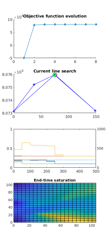
Simple Adjoint Test Using Rate-Control
Generated from simpleRateOpt.m
mrstModule add adjoint mimetic incomp

% whether or not to show output
verbose = false;
verboseLevel = 2;
Define model
nx = 21; ny = 21; nz = 1;
G = cartGrid([nx ny nz], [5*nx 5*ny 1*nz]);
G = computeGeometry(G);

c = G.cells.centroids;
rock.perm  = max(10*sin(c(:,2)/25+.5*cos(c(:,1)/25))-9, .01)*1000*milli*darcy;
rock.poro  = repmat(0.3, [G.cells.num, 1]);

fluid  = initCoreyFluid('mu' , [1, 5] .* centi*poise, ...
                        'rho', [1014, 859].*kilogram/meter^3, ...
                        'n'  , [2, 2], 'sr', [0, 0], 'kwm', [1, 1]);
fluid  = adjointFluidFields(fluid);
Processing Cells   1 : 441 of 441 ... done (0.01 [s], 7.90e+04 cells/second)
Total 3D Geometry Processing Time = 0.006 [s]
Wells and initial rates
radius = .1;
totVol = sum(poreVolume(G, rock));
totTime = 500*day;
W = [];
% Injectors along left side:
nInj = 3; % > 1
pos  = (1 : (ny-1)/(nInj-1) : ny)';
posInj  = round(pos);
for k = 1:nInj
    nm = ['inj', num2str(k)];
    W = addWell(W, G, rock, 1+(posInj(k)-1)*nx, 'Type', 'rate' , 'Val', (1/nInj)*totVol/totTime, ...
                'Radius', radius, 'Name', nm, 'Comp_i', [1, 0], 'Sign', 1, 'InnerProduct', 'ip_tpf');
end
% Producers along right side:
nProd = 5; % >1
pos  = (1 : (ny-1)/(nProd-1) : ny)';
posProd  = round(pos);
for k = 1:nProd
    nm = ['prod', num2str(k)];
    W = addWell(W, G, rock, nx+(posProd(k)-1)*nx, 'Type', 'rate' , 'Val', -(1/nProd)*totVol/totTime, ...
                'Radius', radius, 'Name', nm, 'Comp_i', [1, 0], 'Sign', -1, 'InnerProduct', 'ip_simple');
end
Defaulting reference depth to top of formation for well inj1. Please specify 'refDepth' optional argument to 'addWell' if you require bhp at a specific depth.
Defaulting reference depth to top of formation for well inj2. Please specify 'refDepth' optional argument to 'addWell' if you require bhp at a specific depth.
Defaulting reference depth to top of formation for well inj3. Please specify 'refDepth' optional argument to 'addWell' if you require bhp at a specific depth.
Defaulting reference depth to top of formation for well prod1. Please specify 'refDepth' optional argument to 'addWell' if you require bhp at a specific depth.
Defaulting reference depth to top of formation for well prod2. Please specify 'refDepth' optional argument to 'addWell' if you require bhp at a specific depth.
Defaulting reference depth to top of formation for well prod3. Please specify 'refDepth' optional argument to 'addWell' if you require bhp at a specific depth.
Defaulting reference depth to top of formation for well prod4. Please specify 'refDepth' optional argument to 'addWell' if you require bhp at a specific depth.
Defaulting reference depth to top of formation for well prod5. Please specify 'refDepth' optional argument to 'addWell' if you require bhp at a specific depth.
System components
S = computeMimeticIP(G, rock, 'Type', 'comp_hybrid', 'Verbose', verbose, ...
                     'InnerProduct', 'ip_tpf');
W = assembleWellSystem(G, W, 'Type', 'comp_hybrid');
Initialize
state = initResSol(G, 0.0);
state.wellSol = initWellSol(W, 0);
Objective function
objectiveFunction = str2func('simpleNPV');
Initialize schedule and controls
numSteps = 10;
schedule = initSchedule(W, 'NumSteps', numSteps, 'TotalTime', ...
                        totTime, 'Verbose', verbose);

% box constraints for each well [min rate, max rate]
box = [repmat([0 inf], nInj, 1); repmat([-inf 0], nProd, 1)];
controls = initControls(schedule, 'ControllableWells', (1:numel(W)), ...
                                  'MinMax', box, ...
                                  'Verbose', verbose, ...
                                  'NumControlSteps', numSteps, ...
                                  'LinEqConst', {ones(1, numel(W)), 0}');
Run optimization
simRes, schedule, controls, out] = optimizeObjective(G, S, W, rock, ...
                                        fluid, state, schedule, ...
                                        controls, objectiveFunction, ...
                                        'gradTol',       1e-3, ...
                                        'objChangeTol',  5e-4, ...
                                        'VerboseLevel', verboseLevel);
********** STARTING ITERATION   1 ****************
Current stepsize: -1.00000
----------------- DISPLAYING SCHEDULE ----------------

Time interval :  0.00 - 4320000.00
Well name           Type          Value
     inj1           rate     2.5521e-05
...