`compositional`: Equation-of-state compositional solvers¶

#.. include:: mrst/compositional/README.txt

Models¶

Base classes¶

Contents¶

MODELS

Files: GenericNaturalVariablesModel - GenericOverallCompositionModel - ThreePhaseCompositionalModel - Base class for compositional models

class ThreePhaseCompositionalModel(G, rock, fluid, compFluid, varargin)¶

Bases: ReservoirModel

Base class for compositional models

Synopsis:

model = ThreePhaseCompositionalModel(G, rock, fluid, compFluid)

Description:

This is the base class for several compositional models in MRST. It contains common functionality and is not intended for direct use.

Parameters:	G – Grid structure rock – Rock structure for the reservoir fluid – The flow fluid, containing relative permeabilities, surface densities and flow properties for the aqueous/water phase (if present) compFluid – CompositionalFluid instance describing the species present.
Returns:	model – Initialized class instance

Different formulations¶

Contents¶

NATVARS

Files: equationsNaturalVariables - Equations for natural variables formulation NaturalVariablesCompositionalModel - Natural variables model for compositional problems ReducedLinearizedSystem - Linearized system which performs a Schur complement before solving

class NaturalVariablesCompositionalModel(G, rock, fluid, compFluid, varargin)¶

Bases: ThreePhaseCompositionalModel

Natural variables model for compositional problems

Synopsis:

model = NaturalVariablesCompositionalModel(G, rock, fluid, compFluid)

Description:

The natural variables model relies on separate primary variables for saturations in the multiphase region. This makes it possible to perform certain heuristics to ensure convergence (e.g. saturation chopping) since there is a weaker correspondence between saturations and the compositions. However, this formulation traverses the phase boundary as a number of discrete steps and can take more nonlinear iterations for some problems.

Parameters:	G – Grid structure rock – Rock structure for the reservoir fluid – The flow fluid, containing relative permeabilities, surface densities and flow properties for the aqueous/water phase (if present) compFluid – CompositionalFluid instance describing the species present.
Returns:	model – Initialized class instance

PVT models¶

Equations of state¶

Contents¶

EOS

Files: EquationOfStateModel - Equation of state model. Implements generalized two-parameter cubic EquilibriumConstantModel - Equilibrium constant EOS model for problems where functions of the

class EquationOfStateModel(G, fluid, eosname)¶

Bases: PhysicalModel

Equation of state model. Implements generalized two-parameter cubic equation of state with Newton and successive substitution solvers, as well as standard functions for computing density and viscosity.

computeFugacity(model, p, x, Z, A, B, Si, Bi)¶: Compute fugacity based on EOS coefficients

computeLiquidZ(model, A, B)¶: Pick smallest Z factors for liquid phase (least energy)

computeVaporZ(model, A, B)¶: Pick largest Z factors for vapor phase (most energy)

getMassFraction(model, molfraction)¶: Convert molar fraction to mass fraction

getMixtureFugacityCoefficients(model, P, T, x, y, acf)¶: Calculate intermediate values for fugacity computation

getMoleFraction(model, massfraction)¶: Convert mass fraction to molar fraction

getPhaseFractionAsADI(model, state, p, T, z)¶: Compute derivatives for values obtained by solving the equilibrium equations (molar fractions in each phase, liquid mole fraction).

setZDerivatives(model, Z, A, B, cellJacMap)¶: Z comes from the solution of a cubic equation of state, so the derivatives are not automatically computed. By differentiating the cubic EOS manually and solving for dZ/du where u is some primary variable, we can still obtain derivatives without making any assumptions other than the EOS being a cubic polynomial

solveCubicEOS(model, A, B)¶: Peng Robinson equation of state in form used by Coats

stepFunction(model, state, state0, dt, drivingForces, linsolve, nonlinsolve, iteration, varargin)¶: #ok Compute a single step of the solution process for a given equation of state (thermodynamic flash calculation);

substitutionCompositionUpdate(model, P, T, z, K, L)¶: Determine overall liquid fraction

PropertyModel = None¶: Model to be used for property evaluations

fluid = None¶: CompositionalFluid

minimumComposition = u'1e-8'¶: Minimum composition value (for numerical stability)

omegaA = None¶: Parameter for EOS

omegaB = None¶: Parameter for EOS

selectGibbsMinimum = u'true'¶: Use minimum Gibbs energy to select Z

useNewton = None¶: Use Newton based solver for flash. If set to false, successive substitution if used instead.

class EquilibriumConstantModel(G, fluid, k_values)¶

Bases: EquationOfStateModel

Equilibrium constant EOS model for problems where functions of the type K(p, T, z) is sufficient to describe the phase behavior

Fluid models¶

Contents¶

FLUIDS

Files: BlackOilPropertyModel - Black-oil property model for compositional models CompositionalFluid - CompositionalPropertyModel - Property model for compositional models CoolPropsCompositionalFluid - Create MRST compositional fluid by using the open CoolProp library getCompositionalFluidCase - Grab bag of different fluids for use in examples etc PropertyModel - Base class for properties in the compositional module TableCompositionalFluid - Create MRST compositional from stored tables (taken from CoolProp)

class BlackOilPropertyModel(rho, mu, satfn, varargin)¶

Bases: PropertyModel

Black-oil property model for compositional models

class CompositionalPropertyModel(varargin)¶

Bases: PropertyModel

Property model for compositional models

computeDensity(model, p, x, Z, T, isLiquid)¶: Predict mass density from EOS Z-factor

computeMolarDensity(model, p, x, Z, T, isLiquid)¶: Predict molar density from EOS Z-factor

computePseudoCriticalPhaseProperties(model, x)¶: Molar fraction weighted aggregated properties to get pseudocritical properties of mixture.

computeViscosity(model, P, x, Z, T, isLiquid)¶: Compute viscosity using the Lohrenz, Bray and Clark correlation for hydrocarbon mixtures (LBC viscosity)

class CoolPropsCompositionalFluid(names)¶

Bases: CompositionalFluid

Create MRST compositional fluid by using the open CoolProp library (can be downloaded from http://www.coolprop.org/)

CoolPropsCompositionalFluid(names)¶

Create fluid from names

Synopsis:

f = TableCompositionalFluid({'Methane', 'n-Decane'});

Parameters:	names – Cell array of valid names. See `getFluidList` for valid names.
Returns:	fluid – Initialized fluid.

class PropertyModel(f)¶: Base class for properties in the compositional module

class TableCompositionalFluid(names)¶

Bases: CompositionalFluid

Create MRST compositional from stored tables (taken from CoolProp)

TableCompositionalFluid(names)¶

Create fluid from names

Synopsis:

f = TableCompositionalFluid({'Methane', 'n-Decane'});

Parameters:	names – Cell array of valid names. See `getFluidList` for valid names.
Returns:	fluid – Initialized fluid.

getCompositionalFluidCase(name, varargin)¶: Grab bag of different fluids for use in examples etc

Contents¶

BLACKOIL

Files: blackOilToMassFraction - Evaluate properties convertBlackOilModelToCompositionalModel - Convert blackoil model to compositional-like model convertBlackOilStateToCompositional - Convert BO state to compositional-like state convertRSRVtoKValue - Convert RS/RV b lackoil to K-value. Experimental!

blackOilToMassFraction(model, p, sO, sG, rs, rv)¶: Evaluate properties

convertBlackOilModelToCompositionalModel(bomodel, varargin)¶: Convert blackoil model to compositional-like model

convertBlackOilStateToCompositional(bomodel, state)¶: Convert BO state to compositional-like state

convertRSRVtoKValue(model, varargin)¶: Convert RS/RV b lackoil to K-value. Experimental!

Note

Does not yet support RV.

Examples¶

Example comparing natural variables and overall composition with boundary conditions¶

Generated from compositionalBoundaryConditionsExample.m

We simulate injection of CO2 using boundary conditions and compare two formulations for the same problem in terms of results and nonlinear iterations.

mrstModule add compositional ad-core ad-props

Set up problem¶

nx = 50;
ny = 50;
% Quadratic domain
dims = [nx, ny, 1];
pdims = [1000, 1000, 10];
G = cartGrid(dims, pdims);
G = computeGeometry(G);
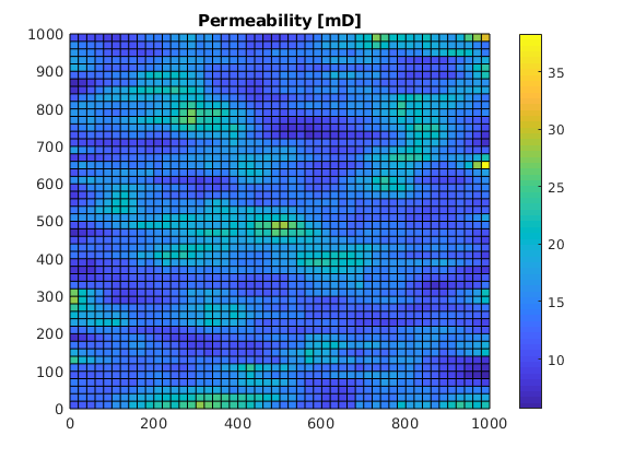
% Generate a random Gaussian permeability field
rng(0);
K = logNormLayers(G.cartDims);
K = K(G.cells.indexMap);
rock = makeRock(G, K*milli*darcy, 0.2);

figure;
plotCellData(G, K);
colorbar;
title('Permeability [mD]');

_images/compositionalBoundaryConditionsExample_01.png

Set up compositional fluid model¶

Three-component system of Methane, CO2 and n-Decane

names = {'Methane'  'CarbonDioxide'  'n-Decane'};
% Critical temperatures
Tcrit = [190.5640 304.1282 617.7000];
% Critical pressure
Pcrit = [4599200 7377300 2103000];
% Critical volumes
Vcrit = [9.8628e-05 9.4118e-05 6.0976e-04];
% Acentric factors
acentricFactors = [0.0114 0.2239 0.4884];
% Mass of components (as MRST uses strict SI, this is in kg/mol)
molarMass = [0.0160 0.0440 0.1423];
% Initialize fluid
fluid = CompositionalFluid(names, Tcrit, Pcrit, Vcrit, acentricFactors, molarMass);

Set up initial state and boundar conditions¶

We inject one pore-volume over 20 years. The right side of the domain is fixed at 75 bar.

minP = 75*barsa;
totTime = 20*year;

pv = poreVolume(G, rock);

bc = [];
bc = fluxside(bc, G, 'xmin', sum(pv)/totTime, 'sat', [1, 0]);
bc = pside(bc, G, 'xmax', minP, 'sat', [1, 0]);

bc.components = repmat([0.1, 0.9, 0], numel(bc.face), 1);

flowfluid = initSimpleADIFluid('rho', [1000, 500, 500], ...
                       'mu', [1, 1, 1]*centi*poise, ...
                       'n', [2, 2, 2], ...
                       'c', [1e-5, 0, 0]/barsa);

ncomp = fluid.getNumberOfComponents();
s0 = [1, 0];
state0 = initResSol(G, 1.5*minP, s0);
T = 423.15;
state0.T = repmat(T, G.cells.num, 1);
state0.components = repmat([0.3000 0.1000 0.6000], G.cells.num, 1);

dt = rampupTimesteps(totTime, 75*day, 12);
schedule = simpleSchedule(dt, 'bc', bc);

Solve with natural variables¶

Natural variables is one possible variable set for compositional problems. These variables include saturations, making it easier to limit updates for problems with strong relative permeability effects.

model = NaturalVariablesCompositionalModel(G, rock, flowfluid, fluid, 'water', false);

nls = NonLinearSolver('useRelaxation', true);
[~, states, report] = simulateScheduleAD(state0, model, schedule, 'nonlinearsolver', nls);

Solving timestep 001/110:          -> 1582 Seconds, 31 Milliseconds
Solving timestep 002/110: 1582 Seconds, 31 Milliseconds -> 3164 Seconds, 62 Milliseconds
Solving timestep 003/110: 3164 Seconds, 62 Milliseconds -> 1 Hour, 2728 Seconds, 125.00 Milliseconds
Solving timestep 004/110: 1 Hour, 2728 Seconds, 125.00 Milliseconds -> 3 Hours, 1856 Seconds, 250.00 Milliseconds
Solving timestep 005/110: 3 Hours, 1856 Seconds, 250.00 Milliseconds -> 7 Hours, 112 Seconds, 500.00 Milliseconds
Solving timestep 006/110: 7 Hours, 112 Seconds, 500.00 Milliseconds -> 14 Hours, 225 Seconds
Solving timestep 007/110: 14 Hours, 225 Seconds -> 1 Day, 4 Hours, 450.00 Seconds
Solving timestep 008/110: 1 Day, 4 Hours, 450.00 Seconds -> 2 Days, 8 Hours, 900.00 Seconds
...

Solve using overall composition¶

Another formulation is to use composition variables with no saturations. In this formulation, the flash is solved between each nonlinear update.

model_o = OverallCompositionCompositionalModel(G, rock, flowfluid, fluid, 'water', false);

[~, states_o, report_o] = simulateScheduleAD(state0, model_o, schedule, 'nonlinearsolver', nls);

Solving timestep 001/110:          -> 1582 Seconds, 31 Milliseconds
Solving timestep 002/110: 1582 Seconds, 31 Milliseconds -> 3164 Seconds, 62 Milliseconds
Solving timestep 003/110: 3164 Seconds, 62 Milliseconds -> 1 Hour, 2728 Seconds, 125.00 Milliseconds
Solving timestep 004/110: 1 Hour, 2728 Seconds, 125.00 Milliseconds -> 3 Hours, 1856 Seconds, 250.00 Milliseconds
Solving timestep 005/110: 3 Hours, 1856 Seconds, 250.00 Milliseconds -> 7 Hours, 112 Seconds, 500.00 Milliseconds
Solving timestep 006/110: 7 Hours, 112 Seconds, 500.00 Milliseconds -> 14 Hours, 225 Seconds
Solving timestep 007/110: 14 Hours, 225 Seconds -> 1 Day, 4 Hours, 450.00 Seconds
Solving timestep 008/110: 1 Day, 4 Hours, 450.00 Seconds -> 2 Days, 8 Hours, 900.00 Seconds
...

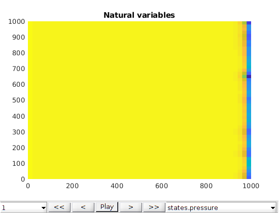
Launch interactive plotting¶

mrstModule add mrst-gui
figure;
plotToolbar(G, states)
title('Natural variables')

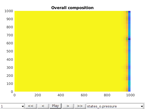
figure;
plotToolbar(G, states_o)
title('Overall composition')

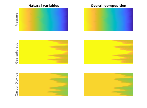
_images/compositionalBoundaryConditionsExample_02.png

_images/compositionalBoundaryConditionsExample_03.png

Plot the pressure, gas saturation and CO2 mole fraction for both solvers¶

We compare the two results and see that they agree on the solution.

[h1, h2, h3, h4, h5, h6] = deal(nan);
h = figure;
for i = 1:numel(states_o)
    figure(h);
    if i > 1
        delete(h1);
        delete(h2);
        delete(h3);
        delete(h4);
        delete(h5);
        delete(h6);
    end
    subplot(3, 2, 1);
    h1 = plotCellData(G, states{i}.pressure, 'EdgeColor', 'none');
    axis tight; set(gca,'xticklabel',[],'yticklabel',[])
    if i == 1
        title('Natural variables')
        ylabel('Pressure')
    end

    subplot(3, 2, 3);
    h3 = plotCellData(G, states{i}.s(:, 2), 'EdgeColor', 'none');
    axis tight; set(gca,'xticklabel',[],'yticklabel',[])
    caxis([0, 1])
    if i == 1
        ylabel('Gas saturation')
    end

    subplot(3, 2, 5);
    h5 = plotCellData(G, states{i}.components(:, 2), 'EdgeColor', 'none');
    axis tight; set(gca,'xticklabel',[],'yticklabel',[])
    caxis([0, 1])
    if i == 1
        ylabel(names{2})
    end

    subplot(3, 2, 2);
    h2 = plotCellData(G, states_o{i}.pressure, 'EdgeColor', 'none');
    if i == 1
        title('Overall composition')
    end
    axis tight; set(gca,'xticklabel',[],'yticklabel',[])

    subplot(3, 2, 4);
    h4 = plotCellData(G, states_o{i}.s(:, 2), 'EdgeColor', 'none');
    axis tight; set(gca,'xticklabel',[],'yticklabel',[])
    caxis([0, 1])

    subplot(3, 2, 6);
    h6 = plotCellData(G, states_o{i}.components(:, 2), 'EdgeColor', 'none');
    axis tight off; set(gca,'xticklabel',[],'yticklabel',[])
    caxis([0, 1])
    drawnow
end

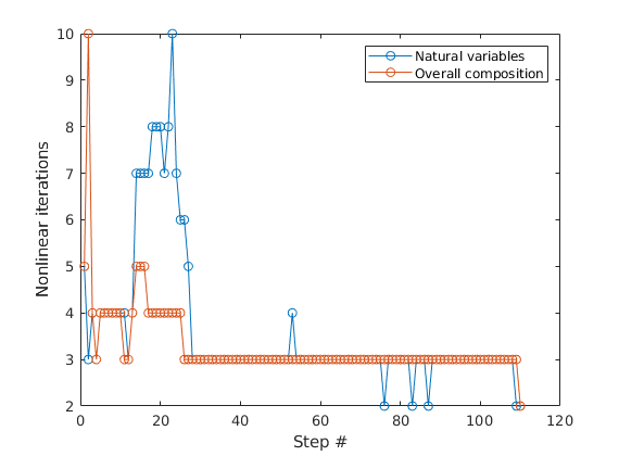
_images/compositionalBoundaryConditionsExample_04.png

Plot the nonlinear iteration count¶

Different solvers are suitable for different problems. In this case, the overall composition model takes slightly fewer iterations.

figure;
plot([report.Iterations, report_o.Iterations], '-o')
legend('Natural variables', 'Overall composition')
xlabel('Step #')
ylabel('Nonlinear iterations')

_images/compositionalBoundaryConditionsExample_05.png

Example demonstrating a three dimensional, six component problem¶

Generated from compositionalExample3DSixComponents.m

We set up a simple grid and rock structure. The numbers can be adjusted to get a bigger/smaller problem. The default is a small problem with 20x20x2 grid blocks.

mrstModule add ad-core ad-props mrst-gui compositional
% Dimensions
nx = 20;
ny = nx;
nz = 2;
% Name of problem and pressure range
casename = 'lumped_1';
minP = 100*barsa;
maxP = 200*barsa;
% Set up grid and rock
dims = [nx, ny, nz];
pdims = [1000, 1000, 1];
G = cartGrid(dims, pdims);
G = computeGeometry(G);
rock = makeRock(G, 50*milli*darcy, 0.25);

Set up quarter five spot well pattern¶

We place vertical wells in opposing corners of the reservoir. The injector is rate controlled and the producer is bottom hole pressure controlled.

W = [];
% Injector
W = verticalWell(W, G, rock, 1, 1, [], 'comp_i', [1, 0], 'name', 'Inj',...
    'Val', 0.0015, 'sign', 1, 'type', 'rate');
% Producer
W = verticalWell(W, G, rock, nx, ny, [], ...
    'comp_i', [0.5, 0.5], 'Name', 'Prod', 'Val', minP, 'sign', -1, 'Type', 'bhp');

Set up model and initial state¶

We set up a problem with quadratic relative permeabilities. The fluid model is retrieved from “High Order Upwind Schemes for Two-Phase, Multicomponent Flow” (SPE 79691) by B. T. Mallison et al. The model consists of six components. Several of the components are not distinct molecules, but rather lumped groups of hydrocarbons with similar molecular weight. The reservoir contains all these components initially, which is then displaced by the injection of pure CO2.

nkr = 2;
[fluid, info] = getCompositionalFluidCase(casename);
flowfluid = initSimpleADIFluid('n', [nkr, nkr, nkr], 'rho', [1000, 800, 10]);

gravity reset on
model = NaturalVariablesCompositionalModel(G, rock, flowfluid, fluid, 'water', false);

ncomp = fluid.getNumberOfComponents();

state0 = initCompositionalState(G, minP + (maxP - minP)/2, info.temp, [0.5, 0.5], info.initial, model.EOSModel);

for i = 1:numel(W)
    W(i).components = info.injection;
end

Set up schedule and simulate the problem¶

We simulate two years of production with a geometric rampup in the timesteps.

time = 2*year;
n = 45;
dt = rampupTimesteps(time, 7*day, 5);
schedule = simpleSchedule(dt, 'W', W);

[ws, states, rep] = simulateScheduleAD(state0, model, schedule);

Solving timestep 001/110:         -> 5 Hours, 900 Seconds
Solving timestep 002/110: 5 Hours, 900 Seconds -> 10 Hours, 1800 Seconds
Solving timestep 003/110: 10 Hours, 1800 Seconds -> 21 Hours
Solving timestep 004/110: 21 Hours -> 1 Day, 18 Hours
Solving timestep 005/110: 1 Day, 18 Hours -> 3 Days, 12 Hours
Solving timestep 006/110: 3 Days, 12 Hours -> 7 Days
Solving timestep 007/110: 7 Days  -> 14 Days
Solving timestep 008/110: 14 Days -> 21 Days
...

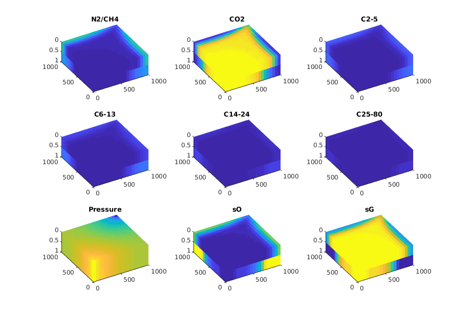
Plot all the results¶

lf = get(0, 'DefaultFigurePosition');
h = figure('Position', lf + [0, -200, 350, 200]);
nm = ceil(ncomp/2);
v = [-30, 60];
for step = 1:numel(states)
    figure(h); clf
    state = states{step};
    for i = 1:ncomp
        subplot(nm, 3, i);
        plotCellData(G, state.components(:, i), 'EdgeColor', 'none');
        view(v);
        title(fluid.names{i})
        caxis([0, 1])
    end
    subplot(nm, 3, ncomp + 1);
    plotCellData(G, state.pressure, 'EdgeColor', 'none');
    view(v);
    title('Pressure')

    subplot(nm, 3, ncomp + 2);
    plotCellData(G, state.s(:, 1), 'EdgeColor', 'none');
    view(v);
    title('sO')

    subplot(nm, 3, ncomp + 3);
    plotCellData(G, state.s(:, 2), 'EdgeColor', 'none');
    view(v);
    title('sG')
    drawnow
end

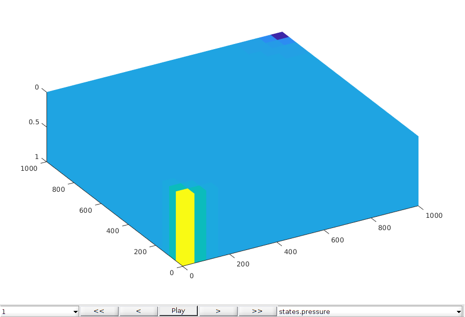
_images/compositionalExample3DSixComponents_01.png

Plot the results in the interactive viewer¶

figure(1); clf;
plotToolbar(G, states)
view(v);
axis tight

_images/compositionalExample3DSixComponents_02.png

Copyright notice¶

<html>
% <p><font size="-1

Conceptual example on how to run larger compositional problems¶

Generated from compositionalLargerProblemTutorial.m

The default settings of the compositional module are suitable for small problems and should work on most configurations with a recent Matlab version. However, with an external linear solver and a change of backend, larger problems can be solved.

mrstModule add compositional ad-core linearsolvers ad-props
useBC = false; % Use BC instead of wells
includeWater = false; % Include aqueous phase
useNatural = true; % Use natural variables formulation
% Define a problem
gravity reset on
nx = 30;
ny = 30;
nz = 30;

dims = [nx, ny, nz];
pdims = [1000, 1000, 100];
G = cartGrid(dims, pdims);
G = computeGeometry(G);
% Random permeability field
rng(0);
K = logNormLayers(G.cartDims);
K = K(G.cells.indexMap);

rock = makeRock(G, K*milli*darcy, 0.2);
pv = poreVolume(G, rock);
% Take the SPE5 fluid model (six components)
[fluid, info] = getCompositionalFluidCase('spe5');

minP = 0.5*info.pressure;
totTime = 10*year;

% Set up driving forces
[bc, W] = deal([]);
if useBC
    bc = fluxside(bc, G, 'xmin', sum(pv)/totTime, 'sat', [0, 1, 0]);
    bc = pside(bc, G, 'xmax', minP, 'sat', [0, 1, 0]);

    bc.components = repmat(info.injection, numel(bc.face), 1);
else
    W = verticalWell(W, G, rock, 1, 1, 1, 'comp_i', [0, 1, 0], ...
        'Type', 'rate', 'name', 'Inj', 'Val', sum(pv)/totTime, 'sign', 1);

    W = verticalWell(W, G, rock, nx, ny, nz, ...
        'comp_i', [0, 0.5, 0.5], 'Name', 'Prod', 'Val', minP, 'sign', -1);


    for i = 1:numel(W)
        W(i).components = info.injection;
    end
end
flowfluid = initSimpleADIFluid('rho', [1000, 500, 500], ...
                       'mu', [1, 1, 1]*centi*poise, ...
                       'n', [2, 2, 2], ...
                       'c', [1e-5, 0, 0]/barsa);

Initialize models¶

We initialize two models: The first uses the standard constructor, and uses the Sparse backend for AD. The second example uses the Diagonal AD backend instead, which is faster for problems with a moderate to many degrees of freedom and several components. The third option is to extended the diagonal backend with C++-acceleration through a mex interface. A compiler must be available (see mex -setup) for this to work. Note that the first simulation with diagonal+mex will occasionally stop to compile subroutines, so the user is encouraged to repeat the benchmark if this is the case. The performance of the backends varies from configuration to configuration, so the user is encouraged to test different versions until the best speed is found.

arg = {G, rock, flowfluid, fluid, 'water', includeWater};
diagonal_backend = DiagonalAutoDiffBackend('modifyOperators', true);
mex_backend = DiagonalAutoDiffBackend('modifyOperators', true, 'useMex', true);
sparse_backend = SparseAutoDiffBackend();

if useNatural
    constructor = @GenericNaturalVariablesModel;
else
    constructor = @GenericOverallCompositionModel;
end

modelSparseAD = constructor(arg{:}, 'AutoDiffBackend', sparse_backend);
modelDiagonalAD = constructor(arg{:}, 'AutoDiffBackend', diagonal_backend);
modelMexDiagonalAD = constructor(arg{:}, 'AutoDiffBackend', mex_backend);

Set up driving forces and initial state¶

ncomp = fluid.getNumberOfComponents();
if includeWater
    s0 = [0.2, 0.8, 0];
else
    s0 = [1, 0];
    for i = 1:numel(W)
        W(i).compi = W(i).compi(2:end);
    end
    if ~isempty(bc)
        bc.sat = bc.sat(:, 2:end);
    end
end
state0 = initCompositionalState(G, info.pressure, info.temp, s0, info.initial, modelSparseAD.EOSModel);

Pick linear solver¶

The AMGCL library is one possible solver option for MRST. It is fairly easy to write interfaces to other solvers using MEX files and/or the LinearSolverAD class. We call the routine for automatically selecting a reasonable linear solver for the specific model.

linsolve = selectLinearSolverAD(modelDiagonalAD);
disp(linsolve)

AMGCL-CPR-block linear solver of class AMGCL_CPRSolverAD
  --------------------------------------------------------
  AMGCL constrained-pressure-residual (CPR) solver. Configuration:
               solver: gmres (Generalized minimal residual method. Parameters: gmres_m. Internal index 4)
       preconditioner: amg (Algebraic multigrid Internal index 1)
           relaxation: ilu0 (Incomplete LU-factorization with zero fill-in - ILU(0). Parameters: ilu_damping. Internal index 3)
           coarsening: aggregation (Aggregation with constant interpolation. Parameters: aggr_eps_strong, aggr_over_interp, aggr_relax. Internal index 3)
         s_relaxation: ilu0 (Incomplete LU-factorization with zero fill-in - ILU(0). Parameters: ilu_damping. Internal index 3)
...

Solve a single short step to benchmark assembly and solve time¶

shortSchedule = simpleSchedule(0.1*day, 'bc', bc, 'W', W);

nls = NonLinearSolver('LinearSolver', linsolve);
[~, statesSparse, reportSparse] = simulateScheduleAD(state0, modelSparseAD, shortSchedule, 'nonlinearsolver', nls);
[~, statesDiagonal, reportDiagonal] = simulateScheduleAD(state0, modelDiagonalAD, shortSchedule, 'nonlinearsolver', nls);
try
    [~, statesMexDiagonal, reportMexDiagonal] = simulateScheduleAD(state0, modelMexDiagonalAD, shortSchedule, 'nonlinearsolver', nls);
catch
    [statesMexDiagonal, reportMexDiagonal] = deal([]);
end

Solving timestep 1/1:                       -> 2 Hours, 1440 Seconds
*** Simulation complete. Solved 1 control steps in 13 Seconds, 469 Milliseconds ***
Solving timestep 1/1:                       -> 2 Hours, 1440 Seconds
*** Simulation complete. Solved 1 control steps in 8 Seconds, 644 Milliseconds ***
Solving timestep 1/1:                       -> 2 Hours, 1440 Seconds
*** Simulation complete. Solved 1 control steps in 5 Seconds, 971 Milliseconds ***

Solve using direct solver¶

This system is too large for the standard direct solver in Matlab. This may take some time!

[~, ~, reportDirect] = simulateScheduleAD(state0, modelSparseAD, shortSchedule);

Solving timestep 1/1:                       -> 2 Hours, 1440 Seconds
*** Simulation complete. Solved 1 control steps in 122 Seconds, 597 Milliseconds ***

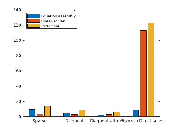
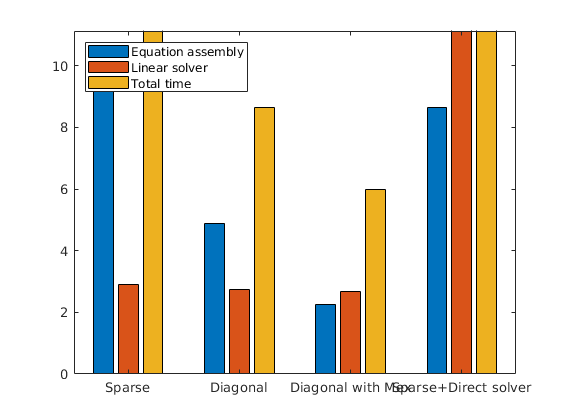
Plot the time taken to solve a single step¶

figure(1 + useNatural); clf

getTime = @(report) [sum(cellfun(@(x) x.AssemblyTime, report.ControlstepReports{1}.StepReports{1}.NonlinearReport)), ...
% Assembly
                     sum(cellfun(@(x) x.LinearSolver.SolverTime, report.ControlstepReports{1}.StepReports{1}.NonlinearReport(1:end-1))),...
% Linear solver
                     sum(report.SimulationTime), ...
                     ];
time_sparse = getTime(reportSparse);
time_diagonal = getTime(reportDiagonal);
time_direct = getTime(reportDirect);
if isempty(reportMexDiagonal)
    time = [time_sparse; time_diagonal; time_direct];
    bar(time)
    set(gca, 'XTickLabel', {'Sparse', 'Diagonal', 'Sparse+Direct solver'});
else
    time_mex = getTime(reportMexDiagonal);
    time = [time_sparse; time_diagonal; time_mex; time_direct];
    bar(time)
    set(gca, 'XTickLabel', {'Sparse', 'Diagonal', 'Diagonal with Mex', 'Sparse+Direct solver'});
end
legend('Equation assembly', 'Linear solver', 'Total time', 'Location', 'NorthWest')

_images/compositionalLargerProblemTutorial_01.png

Zoom in on assembly time¶

assembly_time = time(:, 1);
ylim([0, 1.2*max(assembly_time)]);

_images/compositionalLargerProblemTutorial_02.png

Compare MRST results with other simulators¶

Generated from compositionalValidationSimple.m

This example is a two-phase compositional problem where CO2 is injected into a mixture of CO2, Methane and Decane. The problem consists of 1000 cells and is one dimensional for ease of visualization. The problem is divided into a large number of timesteps to ensure that the different simulators take approximately the same timesteps. The problem is challenging in terms of fluid physics because the pressure is relatively low, which makes the phase behavior highly pressure dependent and all components exist in both phases. Since the wells are set to bottom hole pressure controls, the fluid volume injected is dependent on correctly calculating the mobility and densities in the medium. MRST uses the Peng-Robinson equation of state by default and the Lohrenz, Bray and Clark (LBC) correlation to determine viscosities for both phases.

mrstModule add compositional deckformat ad-core ad-props

Set up model¶

MRST includes both natural variables and overall composition. This toggle can switch between the modes.

useNatural = true;

pth = getDatasetPath('simplecomp');
fn  = fullfile(pth, 'SIMPLE_COMP.DATA');
% Read deck
deck = readEclipseDeck(fn);
deck = convertDeckUnits(deck);
% Set up grid
G = initEclipseGrid(deck);
G = computeGeometry(G);

% Set up rock
rock  = initEclipseRock(deck);
rock  = compressRock(rock, G.cells.indexMap);
fluid = initDeckADIFluid(deck);
% Define some surface densities
fluid.rhoOS = 800;
fluid.rhoGS = 10;

eos = initDeckEOSModel(deck);
if useNatural
    model = NaturalVariablesCompositionalModel(G, rock, fluid, eos.fluid, 'water', false);
else
    model = OverallCompositionCompositionalModel(G, rock, fluid, eos.fluid, 'water', false);
end
schedule = convertDeckScheduleToMRST(model, deck);

% Manually set the injection composition
[schedule.control.W.components] = deal([0, 1, 0]);
% Injection is pure gas
[schedule.control.W.compi] = deal([1, 0]);

Warning: Could not assign property 'STCOND'. Encountered error: 'Undefined
function 'assignSTCOND' for input arguments of type 'struct'.'

Set up initial state¶

The problem is defined at 150 degrees celsius with 75 bar initial pressure. We set up the initial problem and make a call to the flash routines to get correct initial composition.

ncomp = eos.fluid.getNumberOfComponents();

for i = 1:numel(schedule.control.W)
    schedule.control.W(i).lims = [];
end

% Initial conditions
z0 = [0.6, 0.1, 0.3];
T = 150 + 273.15;
p = 75*barsa;

state0 = initCompositionalState(G, p, T, 1, z0, eos);

Simulate the schedule¶

Note that as the poblem has 500 control steps, this may take some time (upwards of 4 minutes).

[ws, states, rep] = simulateScheduleAD(state0, model, schedule);

Solving timestep 001/500:                                -> 864 Seconds
Solving timestep 002/500: 864 Seconds                    -> 2592 Seconds
Solving timestep 003/500: 2592 Seconds                   -> 1 Hour, 2448 Seconds
Solving timestep 004/500: 1 Hour, 2448 Seconds           -> 2 Hours, 2304 Seconds
Solving timestep 005/500: 2 Hours, 2304 Seconds          -> 4 Hours, 2016 Seconds
Solving timestep 006/500: 4 Hours, 2016 Seconds          -> 8 Hours, 1440 Seconds
Solving timestep 007/500: 8 Hours, 1440 Seconds          -> 16 Hours, 288 Seconds
Solving timestep 008/500: 16 Hours, 288 Seconds          -> 1 Day, 2 Hours, 2304.00 Seconds
...

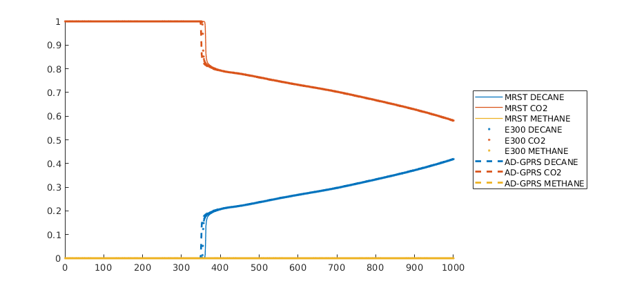
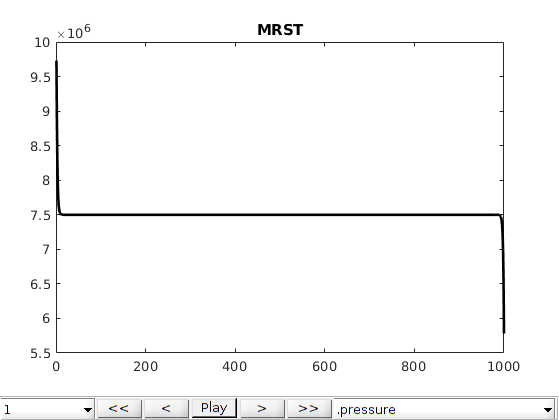
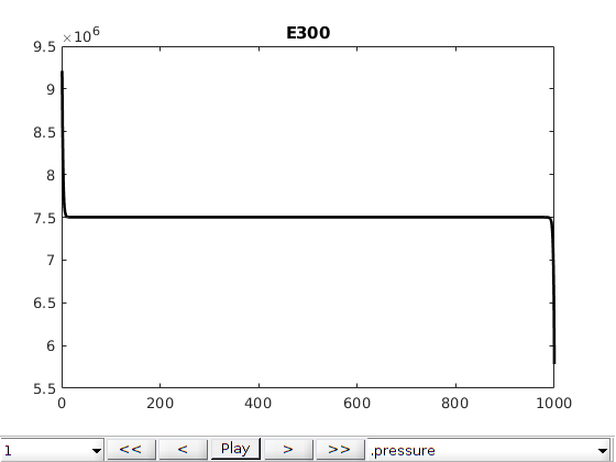
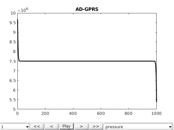
Comparison plots with existing simulators¶

The same problem was defined into two other simulators: Eclipse 300 (which is a commercial simulator) and AD-GPRS (Stanford’s research simulator). We load in precomputed states from these simulators and compare the results. Note that the shock speed is sensitive to the different tolerances in the simulators, which have not been adjusted from the default in either simulator. We observe good agreement between all three simulators, with the minor differences can likely be accounted for by harmonizing the tolerances and sub-timestepping strategy for the different simulators.

lf = get(0, 'DefaultFigurePosition');
h = figure('Position', lf + [0, 0, 350, 0]);
ref = load(fullfile(pth, 'comparison.mat'));
data = {states, ref.statesECL, ref.statesGPRS};
n = min(cellfun(@numel, data));
names = {'MRST', 'E300', 'AD-GPRS'};
markers = {'-', '.', '--'};
cnames = model.EOSModel.fluid.names;

nd = numel(data);
l = cell(nd*ncomp, 1);
for i = 1:nd
    for j = 1:ncomp
        l{(i-1)*ncomp + j} = [names{i}, ' ', cnames{j}];
    end
end
lw = [1, 2, 2];
colors = lines(ncomp);
for step = 1:n
    figure(h); clf; hold on
    for i = 1:numel(data)
        s = data{i}{step};
        comp = s.components;
        if iscell(comp)
            comp = [comp{:}];
        end
        for j = 1:ncomp
            plot(comp(:, j), markers{i}, 'linewidth', lw(i), 'color', colors(j, :));
        end
    end
    legend(l, 'location', 'eastoutside');
    ylim([0, 1]);
    drawnow
end

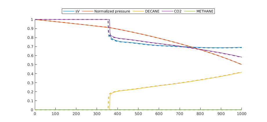
_images/compositionalValidationSimple_01.png

Compare pressure and saturations¶

We also plot a more detailed comparison between MRST and E300 to show that the prediction of phase behavior is accurate.

colors = lines(ncomp + 2);
for step = 1:n
    figure(h); clf; hold on
    for i = 1:2
        s = data{i}{step};
        if i == 1
            marker = '-';
            linewidth = 1;
        else
            marker = '--';
            linewidth = 2;
        end
        hs = plot(s.s(:, 2), marker, 'color', [0.913, 0.172, 0.047], 'linewidth', linewidth, 'color', colors(1, :));
        p = s.pressure./max(s.pressure);
        hp = plot(p, marker, 'linewidth', linewidth, 'color', colors(2, :));
        comp = s.components;
        if iscell(comp)
            comp = [comp{:}];
        end

        if i == 1
            handles = [hs; hp];
        end
        for j = 1:ncomp
            htmp = plot(comp(:, j), marker, 'linewidth', linewidth, 'color', colors(j + 2, :));
            if i == 1
                handles = [handles; htmp];
            end
        end
        if i == 2
            legend(handles, 'sV', 'Normalized pressure', cnames{:}, 'location', 'northoutside', 'orientation', 'horizontal');
        end
    end
    ylim([0, 1]);
    drawnow
end

_images/compositionalValidationSimple_02.png

Set up interactive plotting¶

Finally we set up interactive plots to make it easy to look at the results from the different simulators.

mrstModule add mrst-gui
for i = 1:nd
    figure;
    plotToolbar(G, data{i}, 'plot1d', true);
    title(names{i});
end

_images/compositionalValidationSimple_03.png

_images/compositionalValidationSimple_04.png

_images/compositionalValidationSimple_05.png

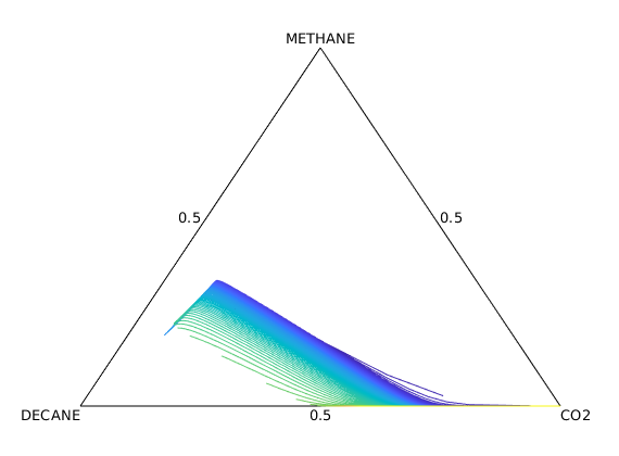
Plot displacement lines in ternary diagram¶

figure; hold on
plot([0, 0.5, 1, 0], [0, sqrt(3)/2, 0, 0], 'k')


mapx = @(x, y, z) (1/2)*(2*y + z)./(x + y+ z);
mapy = @(x, y, z) (sqrt(3)/2)*z./(x + y+ z);

colors = parula(numel(states));
for i = 1:5:numel(states)
    C = states{i}.components;
    plot(mapx(C(:, 1), C(:, 2), C(:, 3)), mapy(C(:, 1), C(:, 2), C(:, 3)), '-', 'color', colors(i, :))

end
axis off

text(0, 0, model.EOSModel.fluid.names{1}, 'verticalalignment', 'top', 'horizontalalignment', 'right')
text(1, 0, model.EOSModel.fluid.names{2}, 'verticalalignment', 'top', 'horizontalalignment', 'left')
text(0.5, sqrt(3)/2, model.EOSModel.fluid.names{3}, 'verticalalignment', 'bottom', 'horizontalalignment', 'center')


text(mapx(0.5, 0.5, 0), mapy(0.5, 0.5, 0), '0.5', 'verticalalignment', 'top', 'horizontalalignment', 'center')
text(mapx(0, 0.5, 0.5), mapy(0, 0.5, 0.5), '0.5', 'verticalalignment', 'bottom', 'horizontalalignment', 'left')
text(mapx(0.5, 0.0, 0.5), mapy(0.5, 0.0, 0.5), '0.5', 'verticalalignment', 'bottom', 'horizontalalignment', 'right')

_images/compositionalValidationSimple_06.png

Example demonstrating compositional solvers with K-values¶

Generated from runCompositionalSPE1.m

We solve SPE1 using two compositional models with the black-oil properties represented as pressure and composition-dependent equilibrium constants.

First, setup the base case¶

mrstModule add ad-core ad-blackoil compositional ad-props mrst-gui
[G, rock, fluid, deck, state] = setupSPE1();

model = ThreePhaseBlackOilModel(G, rock, fluid, 'disgas', true);
model.extraStateOutput = true;
schedule = convertDeckScheduleToMRST(model, deck);

Switch well limits¶

The compositional solvers use a different definition of oil-rate controls. For this reason, we adjust the control of the producer to use BHP.

schedule.control.W(2).type = 'bhp';
schedule.control.W(2).val = 200*barsa;
schedule.control.W(2).lims = [];

Convert state and wells¶

state0 = convertBlackOilStateToCompositional(model, state);
for i = 1:numel(schedule.control(1).W)
    schedule.control(1).W(i).components = schedule.control(1).W(i).compi(2:end);
end

Convert model to compositional model¶

This is based on interpolation and is not completely robust.

modelNat = convertBlackOilModelToCompositionalModel(model, 'interpolation', 'pchip');
modelNat.FacilityModel = FacilityModel(modelNat);
modelNat.FacilityModel.toleranceWellRate = 1e-3;
modelNat.dsMaxAbs = 0.2;
modelNat.dzMaxAbs = inf;
modelNat.incTolPressure = inf;

Run natural variables¶

[wsNat, statesNat, reportNat] = simulateScheduleAD(state0, modelNat, schedule);

Solving timestep 001/120:                   -> 1 Day
Solving timestep 002/120: 1 Day             -> 3 Days
Solving timestep 003/120: 3 Days            -> 5 Days
Solving timestep 004/120: 5 Days            -> 10 Days
Solving timestep 005/120: 10 Days           -> 15 Days
Solving timestep 006/120: 15 Days           -> 25 Days
Solving timestep 007/120: 25 Days           -> 35 Days
Solving timestep 008/120: 35 Days           -> 45 Days
...

Run overall composition¶

modelOverall = OverallCompositionCompositionalModel(G, rock, fluid, modelNat.EOSModel);
modelOverall.FacilityModel = FacilityModel(modelOverall);
modelOverall.FacilityModel.toleranceWellRate = modelNat.FacilityModel.toleranceWellRate;

modelOverall.dsMaxAbs = modelNat.dsMaxAbs;
modelOverall.dzMaxAbs = modelNat.dzMaxAbs;
modelOverall.incTolPressure = modelNat.incTolPressure;


[wsOverall, statesOverall, reportOverall] = simulateScheduleAD(state0, modelOverall, schedule);

Solving timestep 001/120:                   -> 1 Day
Solving timestep 002/120: 1 Day             -> 3 Days
Solving timestep 003/120: 3 Days            -> 5 Days
Solving timestep 004/120: 5 Days            -> 10 Days
Solving timestep 005/120: 10 Days           -> 15 Days
Solving timestep 006/120: 15 Days           -> 25 Days
Solving timestep 007/120: 25 Days           -> 35 Days
Solving timestep 008/120: 35 Days           -> 45 Days
...

Run the reference¶

model.FacilityModel = FacilityModel(model);
model.FacilityModel.toleranceWellRate = modelNat.FacilityModel.toleranceWellRate;

[wsRef, statesRef, reportRef] = simulateScheduleAD(state, model, schedule);

Solving timestep 001/120:                   -> 1 Day
Solving timestep 002/120: 1 Day             -> 3 Days
Solving timestep 003/120: 3 Days            -> 5 Days
Solving timestep 004/120: 5 Days            -> 10 Days
Solving timestep 005/120: 10 Days           -> 15 Days
Solving timestep 006/120: 15 Days           -> 25 Days
Solving timestep 007/120: 25 Days           -> 35 Days
Solving timestep 008/120: 35 Days           -> 45 Days
...

Store component rates for the reference solution in the same format¶

for i = 1:numel(wsRef)
    for j = 1:numel(wsRef{i})
        wsRef{i}(j).PseudoGas = wsRef{i}(j).qGs.*fluid.rhoGS;
        wsRef{i}(j).PseudoOil = wsRef{i}(j).qOs.*fluid.rhoOS;
    end
end

Add interactive plotting¶

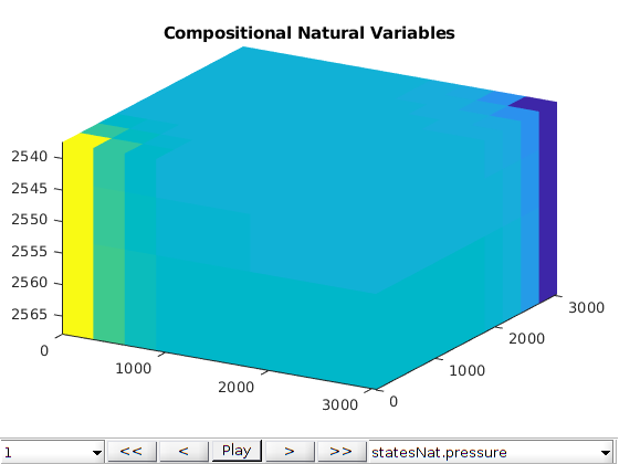
Note: Gas and oil rates in the producer are defined differently between the solvers, and will not match

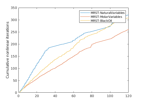
names = {'MRST-NaturalVariables', 'MRST-MolarVariables', 'MRST-BlackOil'};
figure;
plotToolbar(G, statesNat);
title('Compositional Natural Variables')
axis tight
view(30, 30);
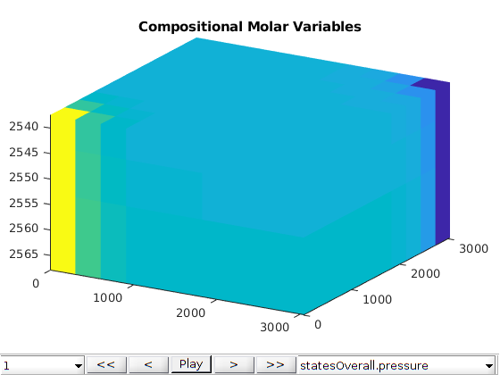
figure;
plotToolbar(G, statesOverall);
title('Compositional Molar Variables')
axis tight
view(30, 30);

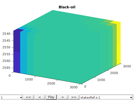
figure;
plotToolbar(G, statesRef);
title('Black-oil');
axis tight
view(30, 30);
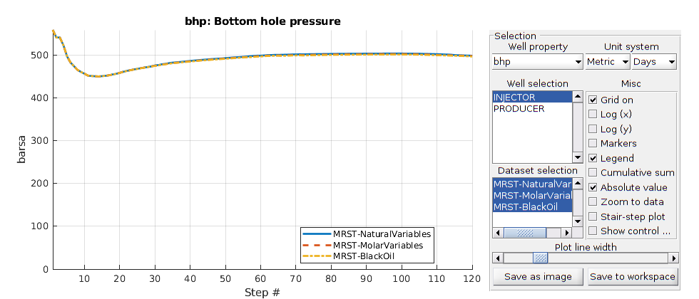
plotWellSols({wsNat, wsOverall, wsRef}, 'datasetnames', names)

Plot nonlinear iterations¶

figure;
stairs(cumsum([reportNat.Iterations, reportOverall.Iterations, reportRef.Iterations]));
legend(names);
ylabel('Cumulative nonlinear iterations')

compositional: Equation-of-state compositional solvers¶

Models¶

Base classes¶

Different formulations¶

PVT models¶

Equations of state¶

Fluid models¶

Examples¶

Example comparing natural variables and overall composition with boundary conditions¶

Set up problem¶

Set up compositional fluid model¶

Set up initial state and boundar conditions¶

Solve with natural variables¶

Solve using overall composition¶

Launch interactive plotting¶

Plot the pressure, gas saturation and CO2 mole fraction for both solvers¶

Plot the nonlinear iteration count¶

Example demonstrating a three dimensional, six component problem¶

Set up quarter five spot well pattern¶

Set up model and initial state¶

Set up schedule and simulate the problem¶

Plot all the results¶

Plot the results in the interactive viewer¶

Copyright notice¶

Conceptual example on how to run larger compositional problems¶

Initialize models¶

Set up driving forces and initial state¶

Pick linear solver¶

Solve a single short step to benchmark assembly and solve time¶

Solve using direct solver¶

Plot the time taken to solve a single step¶

Zoom in on assembly time¶

Compare MRST results with other simulators¶

Set up model¶

Set up initial state¶

Simulate the schedule¶

Comparison plots with existing simulators¶

Compare pressure and saturations¶

Set up interactive plotting¶

Plot displacement lines in ternary diagram¶

Example demonstrating compositional solvers with K-values¶

First, setup the base case¶

Switch well limits¶

Convert state and wells¶

Convert model to compositional model¶

Run natural variables¶

Run overall composition¶

Run the reference¶

Store component rates for the reference solution in the same format¶

Add interactive plotting¶

Plot nonlinear iterations¶

`compositional`: Equation-of-state compositional solvers¶