`heterogeneity`¶

computeDTOF(G, rock, fluid, comp, startCells, cellSize)¶

Compute diffusive time of flight with Fast Marching Method (FMM). See Zhang et al. 2013 (SPE 163637). The diffusive time of flight is related to the propagation of a pressure front, similar to the depth of investigation.

Synopsis:

DTOF = computeDTOF(G,rock,fluid,comp,startCells,cellSize)

Parameters:

G – Cartesian or logically Cartesian grid.
rock – Rock structure with the fields ‘poro’ and ‘perm’.
fluid – MRST fluid structure where fluid.properties(1)=viscosity
comp – Total compressibility. Vector of size (1,1) or (N,1) where N is the number of grid cells.
startCells – Cells where DTOF=0;
cellSize – Vector of size (1,d) or (N,d) where d is dimension of the grid and N is the number of cells.

Returns:

DTOF – Diffusive time of flight
Written by Asgeir Nyvoll, MSc student NTNU, 2018

effPermDesc(BS, CS, TauS2, QS, Ve)¶

Calculate effective permeability descriptors from streamline descriptors effective bulk volume and rates

SYNOPSIS: [BS, CS, TauS2]=streamtubePermDesc(GradP, LS, fluid, shortestpath);

Parameters:	GradP – Pressure gradients for each substep in Pollock approximation LS – Streamline length for each substep in Pollock approximation fluid – MRST fluid structure where fluid.properties(1) is viscosity shortestpath – Length of streamline if no tortuosity
Returns:	BS – Streamline/streamtube hydraulic conductance CS – Streamline constriction factor TauS2 – Streamline tortuosity factor

EXAMPLE:

[BS, CS, TauS2]=streamtubePermDesc(GradP, LS, fluid, shortestpath);

SEE ALSO: effPermDesc(), pollockMod() Written by Asgeir Nyvoll, MSc student NTNU, 2018

pollockMod(G, state, rock, varargin)¶

Trace streamlines in logically Cartesian grid using Pollock approximation. In addition to the regular Pollock approximation, pressure gradients are supported.

Synopsis:

[S,T,C,L,V,GP] = pollockMod(G, state, rock)
[S,T,C,L,V,GP] = pollockMod(G, state, rock, startpos)
[S,T,C,L,V,GP] = pollockMod(G, state, rock, 'pn', pv, ...)
[S,T,C,L,V,GP] = pollockMod(G, state, rock, startpos, 'pn', pv, ...)

Parameters:	G – Cartesian or logically Cartesian grid. state – State structure with field ‘flux’. rock – Rock structure with the field ‘poro’.

OPTIONAL PARAMETERS

positions - Matrix of size (N, 1) or (N, d+1), where d is the dimension

of the grid, used to indicate where the streamlines should start.

If the size is (N, 1), positions contains the cell indices in which streamlines should start. Each streamline is started in the the local coordinate (0.5, 0.5, …). To be precise, this is the mean of the corner points, not the centroid of the cell.

If the size is (N, d+1), the first column contains cell indices, and the d next columns contain the local coordinates at which to start streamlines.

OPTIONAL PARAMETERS (supplied in ‘key’/value pairs (‘pn’/pv …)):

substeps - Number of substeps in each cell, to improve visual quality.

Default 5.

maxsteps - Maximal number of points in a streamline.

Default 1000.

reverse - Reverse velocity field before tracing.

Default false.

periodic - Grid with periodic boundary conditions.

Default not periodic boundary conditions.

fluid - MRST fluid structure where fluid.properties(1)=viscosity

Default viscosity: 1 cP

lineLength - Method for streamline length calculation. Options:

‘straight’ (straight line between plots) and ‘integral’. Default: ‘straight’

Returns:	S – Cell array of individual streamlines suitable for calls like streamline(pollock(…)) and streamtube(pollock(…)). T – Time-of-flight of coordinate. C – Cell number of streamline segment, i.e, line segment between two streamline coordinates. L – Streamline lengths V – Velocity vectors GP – Pressure gradients

Example:

[S,T,C,L,V,GP] = pollockMod(G, x, rock,startpos,'fluid',fluid);

streamline(S);

Examples¶

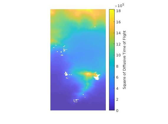
Example script of diffusive time of flight¶

Generated from diffusiveTimeOfFlightFMM.m

Example of diffusive time of flight for a horizontal layer of the SPE10 model. The computeDTOF function is an implementation of the Fast Marching Method (FMM) for diffusive time of flight as presented in Zhang et al. 2013 (SPE 163637)

User defined variables¶

%Fluid
viscosity           = 1*centi*poise;
density             = 1014*kilogram/meter^3;
compressibility     = 4.4e-10;

Load necessary MRST modules¶

mrstModule add spe10 heterogeneity incomp

load SPE10 - data, will attempt to download if not available locally¶

[G, W, rock] = getSPE10setup(30); % Loads layer
rock.perm(rock.poro==0,:) = 0; % To fix positive perm in deactivated cells.

Line-drive bottom to top¶

[nx, ny] = deal(G.cartDims(1), G.cartDims(2));
bottomCells = (1:nx)';
topCells    = (1:nx)' + nx*(ny-1);

Fluid structure¶

fluid       = initSingleFluid('mu' ,    viscosity, 'rho', density);

Calculating cell sizes¶

Rectangular cuboids are assumed. In this case all cells are equal, and we could simply set cellSize = [6.096 3.048 0.6096] and get the same result.

cellNo      = rldecode(1:G.cells.num, diff(G.cells.facePos), 2) .';
cf          = accumarray([cellNo, G.cells.faces(:,2)], G.cells.faces(:,1));
gc          = G.faces.centroids;
cellSize    = [gc(cf(:,2),1)-gc(cf(:,1),1) gc(cf(:,4),2)-gc(cf(:,3),2) ...
                gc(cf(:,6),3)-gc(cf(:,5),3)];
clear cf gc cellNo

Calculate diffusive time of flight¶

dtof=computeDTOF(G,rock,fluid,compressibility,bottomCells,cellSize);

Plotting diffusive time of flight¶

The square is plotted as the units of “diffusive time of flight” as is square root of time.

figure(1), plotCellData(G, dtof.^2,...
 'Edgecolor', 'none', 'FaceAlpha', .6) ;
c=colorbar;
c.Label.String = 'Square of Diffusive Time of Flight';
axis off tight equal

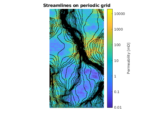
Example script with Pollock algorithm on periodic grid¶

Generated from periodicPollockStreamlines.m

The pollockMod function is an expansion and modification of the regular pollock algorithm in MRST. This example is with a periodic grid in the x-direction of a single layer of the SPE10 model. NB: Add ‘Gp.faces.areas=Gp.faces.areas(1:Gp.faces.num);’ at the end of ‘makePeriodicGridMulti3D’ in the ‘upscaling’ module to fix problem with too many values in ‘Gp.faces.areas’.

User-defined variables¶

%Streamlines
streamlinesPerCell  = 1;
nsubsteps           = 10;
linelength         = 'integral'; %Length estimation method

% Boundary Conditions
pIn                 = 500*barsa();
pOut                = 100*barsa();

%Fluid
viscosity           = 1*centi*poise;
density             = 1014*kilogram/meter^3;

% rateLimit: since the solver can give very small positive
% rates in cells that are enclosed by no flow cells, but still has positive
% permeability themselves. We want to avoid that streamlines can start in
% such cells. (eps is the floating point relative accuracy of Matlab)

rateLimit           = 100*eps; % Cutoff for "active cells"

Load necessary MRST modules¶

mrstModule add spe10 incomp heterogeneity upscaling

load SPE10 - data, will attempt to download if not available locally¶

[G, W, rock] = getSPE10setup(30); % Loads layer
is_pos = rock.poro > 0;
rock.poro(~is_pos) = min(min(rock.poro(is_pos)) / 100, 1.0e-6);

Periodic boundaries¶

Periodic in x-direction

bcr{1}=pside([],G,'RIGHT',0);   bcl{1}=pside([],G,'LEFT',0);

Constant pressure boundaries: Linedrive bottom-to-top¶

Constant pressure at y-direction boundaries (z-direction is no-flow)

[nx, ny] = deal(G.cartDims(1), G.cartDims(2));
bottomCells = (1:nx)';
topCells    = (1:nx)' + nx*(ny-1);
%Make periodic grid
[Gp, bcp]=makePeriodicGridMulti3d(G, bcl, bcr, {0});
bc = pside([],Gp,'YMin',pIn);
bc = pside(bc,Gp,'YMax',pOut);

Initialization of periodic grid¶

T       = computeTransGp(G, Gp, rock);
fluid   = initSingleFluid('mu' ,    viscosity, ...
                           'rho', density);
initState = initResSol(Gp, 0.0);

Solve incompTPFA to get steady-state pressure solution¶

sol = incompTPFA(initState, Gp, T, fluid, 'bc', bc,'bcp',bcp);

Warning: Face pressures are not well defined for periodic boundary faces

Find flux in each cell to compare with the rate limit¶

sol.flux(isnan(sol.flux))=0;    %Fix NaN

cellNo = rldecode(1:Gp.cells.num, diff(Gp.cells.facePos), 2) .';
   cf     = Gp.cells.faces;
   flux= accumarray([cellNo, cf(:,2)], sol.flux(cf(:,1)));
   clear cf cellNo
   flux(:,2:2:end)=-1*flux(:,2:2:end);
cellFluxSum=sum(flux,2);
cellFlux=sum(flux.*(flux>0),2);

Compute start positions for streamlines¶

startCells = repmat(bottomCells,1,streamlinesPerCell);
startCells = reshape(startCells',[],1);
startPosLoc = [zeros(length(startCells),2), ones(length(startCells),1).*0.5];
startStep = 1/streamlinesPerCell; % Streamline spacing in start cell
                                  % in unit cell coordinates for pollock()
first = startStep/2;       % Unit cell coordinate first streamline in cell
last = 1-first;            % Unit cell coordinate first streamline in cell
startPosLoc(:,1)=repmat((first:startStep:last)',length(bottomCells),1);
startPos = [startCells, startPosLoc];

% Finds active start cells
active=cellFlux(startCells)>rateLimit;

[S, T, C]=pollockMod(G, sol,rock,startPos(active,:), ...
    'substeps', nsubsteps ,'maxsteps', 4e5,'fluid',fluid, 'periodic', Gp, 'lineLength',linelength);

figure(1), plotCellData(G, log(convertTo(rock.perm(:,2),milli*darcy)),...
 'Edgecolor', 'none', 'FaceAlpha', .6)
c=colorbar('Ticks',log([0.01,0.1,1,10,100,1000,10000]), 'TickLabels',...
{'0.01', '0.1','1','10','100','1000','10000'});
c.Label.String = 'Permeability [mD]';
title 'Streamlines on periodic grid'
axis off tight equal

% Plot streamlines if wanted (choose figure number from the plots above)
figure(1), h = streamline(S);
set(h, 'Color', 'black', 'LineStyle', 'none', 'Marker', '.', 'MarkerSize', 3)
% increase z to plot streamlines above perm-field
for k =1:numel(h)
    h(k).ZData = h(k).ZData - 10;
end

_images/periodicPollockStreamlines_01.png

Example script calculating permeability descriptors¶

Generated from permeabilityDescrModel.m

Model described in Nyvoll (2017) and Nyvoll (2018), which is a specialization project and a master thesis, respectively. (Both currently unpublished as of June 2018)

User-defined variables¶

%Streamlines
streamlinesPerCell  = 20;
nsubsteps           = 10;
linelength         = 'straight';
% Boundary Conditions
pIn                 = 500*barsa();
pOut                = 100*barsa();

%Fluid
viscosity           = 1*centi*poise;
density             = 1014*kilogram/meter^3;

% rateLimit: since the solver can give very small positive
% rates in cells that are enclosed by no flow cells, but still has positive
% permeability themselves. eps is the floating point relative accuracy
% of Matlab

rateLimit           = 100*eps; % Cutoff for "active cells"

Load necessary MRST modules¶

mrstModule add spe10 incomp heterogeneity

load SPE10 - data, will attempt to download if not available locally¶

layerNum = 1;  % choose layer
[G, W, rock] = getSPE10setup(layerNum); % Loads layer
rock.perm(rock.poro==0,:)=0; % To fix positive perm in deactivated cells.

Constant pressure boundaries: Linedrive bottom-to-top¶

[nx, ny] = deal(G.cartDims(1), G.cartDims(2));
bottomCells = (1:nx)';
topCells    = (1:nx)' + nx*(ny-1);
bc = pside([],G,'YMin',pIn);
bc = pside(bc,G,'YMax',pOut);

Computing Transmissibilities, fluid and create initial state¶

T       = computeTrans(G, rock);
fluid   = initSingleFluid('mu' ,    viscosity, ...
                           'rho', density);
 initState = initResSol(G, 0.0);

Solve incompTPFA to get steady-state pressure solution¶

sol = incompTPFA(initState, G, T, fluid, 'bc', bc);

Warning: Matrix is singular to working precision.

Find cell fluxes to compare with rate limit¶

sol.flux(isnan(sol.flux))=0;    %Fix NaN
cellNo = rldecode(1:G.cells.num, diff(G.cells.facePos), 2) .';
   cf     = G.cells.faces;
   flux= accumarray([cellNo, cf(:,2)], sol.flux(cf(:,1)));
   clear cf cellNo
   flux(:,2:2:end)=-1*flux(:,2:2:end);
cellFluxSum=sum(flux,2);
cellFlux=sum(flux.*(flux>0),2);

Compute start positions for streamlines¶

Using equal spacing at each inlet face.

startCells = repmat(bottomCells,1,streamlinesPerCell);
startCells = reshape(startCells',[],1);
startPosLoc = [zeros(length(startCells),2), ones(length(startCells),1).*0.5];
startStep = 1/streamlinesPerCell; % Streamline spacing in start cell
                                  % in unit cell coordinates for pollockMod()
first = startStep/2;       % Unit cell coordinate first streamline in cell
last = 1-first;            % Unit cell coordinate first streamline in cell
startPosLoc(:,1)=repmat((first:startStep:last)',length(bottomCells),1);
startPos = [startCells, startPosLoc];

% Finds active start cells
active=cellFlux(startCells)>rateLimit;

Modified pollock method¶

Uses all possible outputs of pollockMod, including (in order): coordinates, times of flight, current cell, streamline step lengths, velocity vectors and pressure gradients based on 1D darcy flow along each streamline.

[S, T, C,LS,VXYZ,GradP]=pollockMod(G, sol,rock,startPos(active,:), ...
    'substeps', nsubsteps ,'maxsteps', 4e5,'fluid',fluid, 'lineLength',linelength);

Various calculations¶

Rate for each streamtube around streamlines:

Qs=ones(size(S)).*flux(startCells(active),3)./streamlinesPerCell;

% Total rate
Q=sum(Qs);

%Bulk volume
V=sum(G.cells.volumes);

% Effective bulk volume
Ve=sum(G.cells.volumes(cellFlux>rateLimit));

% Pore Volume
OmegaS=sum(sum(poreVolume(G,rock)));

% Find number of streamlines started in active cells:
nstreamlines=length(S);
BS=zeros(nstreamlines,1);
CS=BS;
TauS2=BS;
% Model length in main flow direction (y-direction).
Ltot=max(G.faces.centroids(:,2))-min(G.faces.centroids(:,2));

Streamline/streamtube permeability descriptors¶

for i=1:nstreamlines
   [BS(i), CS(i), TauS2(i)]=streamtubePermDesc(GradP{i}, LS{i}, fluid, 670.56);
   % BS streamline conductance, CS streamline constriction factor and TauS2
   % streamline tortuoisty factor.
end
tof=zeros(length(T),1);
for i = 1 : length(T)
    % Time of flight /residence time of each streamline
    tof(i,1)=sum(T{i}(:));
end

Effective layer permeability descriptors and variance¶

[Be,Ce,Te2,varTs2,varInvCs]= ...
    effPermDesc(BS,CS,TauS2, Qs, Ve);

Permeability¶

%ke calculated with Darcy over full layer
keff=-Q*fluid.properties(1)*670.56/...
    (-4e7*sum(G.faces.areas(13421:13480)));
%Average k_h in V (k_x=k_y=k_h)
kavg=mean(rock.perm(:,2));
%Average k_h in Ve (for spe10: Should equal Be)
kavgact=mean(rock.perm(cellFlux>rateLimit,2));
%ke calculated with effective descriptors from streamlines
keffs=Te2*Be*Ve/(Ce*V);

heterogeneity¶

Examples¶

Example script of diffusive time of flight¶

User defined variables¶

Load necessary MRST modules¶

load SPE10 - data, will attempt to download if not available locally¶

Line-drive bottom to top¶

Fluid structure¶

Calculating cell sizes¶

Calculate diffusive time of flight¶

Plotting diffusive time of flight¶

Example script with Pollock algorithm on periodic grid¶

User-defined variables¶

Load necessary MRST modules¶

load SPE10 - data, will attempt to download if not available locally¶

Periodic boundaries¶

Constant pressure boundaries: Linedrive bottom-to-top¶

Initialization of periodic grid¶

Solve incompTPFA to get steady-state pressure solution¶

Find flux in each cell to compare with the rate limit¶

Compute start positions for streamlines¶

Example script calculating permeability descriptors¶

User-defined variables¶

Load necessary MRST modules¶

load SPE10 - data, will attempt to download if not available locally¶

Constant pressure boundaries: Linedrive bottom-to-top¶

Computing Transmissibilities, fluid and create initial state¶

Solve incompTPFA to get steady-state pressure solution¶

Find cell fluxes to compare with rate limit¶

Compute start positions for streamlines¶

Modified pollock method¶

Various calculations¶

Streamline/streamtube permeability descriptors¶

Effective layer permeability descriptors and variance¶

Permeability¶

`heterogeneity`¶