agglom: Flow and property-based coarse-grid generation

The module consists of a set of modular components that can be combined in different ways to create coarse grids that adapt to geology and flow fields. The fundamental characteristic of all algorithms is that coarse blocks are generated by amalgamating cells from the original fine grid, with cell-wise indicator functions guiding the amalgamation directions and the new grid resolution.

See the ‘coarsegrid’ module for simpler partition methods and data structures for representing coarse grids.

Utilities

Contents

NUC Support for non-uniform coarsening/agglomeration method

Files

applySuccessivePart - Refine blocks by successively applying static background partitions mergeBlocks - Merge blocks in a partitioning that are smaller than the given limit. mergeBlocks2 - Alternative implementation of Amalgamation ‘MERGE’ primitive refineBlocks - Refine blocks for which indicator value exceeds given limit refineGreedy - Refine blocks in a partition using a greedy algorithm refineGreedy2 - Refine blocks in a partition using a greedy algorithm refineGreedy3 - Refine blocks in a partition using a greedy algorithm refineGreedy4 - Refine blocks in a partition using a greedy algorithm refineRecursiveCart - Refine blocks by recursively applying Cartesian refinement pattern refineUniform - Refine blocks in a partition by uniform partitioning refineUniformShape - Refine blocks in a partition segmentIndicator - Segments a fine grid into blocks according to indicator.

applySuccessivePart(p, G, indicator, NU, pfixed)

Refine blocks by successively applying static background partitions

Synopsis:

p = applySuccessivePart(p, G, I, NU, pf)

Description:

Given a partition ‘p’ of a grid ‘G’, this function applies a set of fixed subdivisions pf(:,1) to pf(:,end) successively to coarse blocks in the grid. In each block, the next subdivision in the succession is only applied if the accumulative indicator inside the block exceeds a prescribed threshold. The indicator function ‘I’ is interpreted as a density and multiplied by the cell volume to derive the total indicator value for each cell. No block should have a total accumulated indicator value exceeding “NU / G.cells.num” times the total accumulated indicator value for the whole grid,

SUM(I .* G.cells.volumes)

Parameters:

• p – Partition vector.
• G – Grid data structure
• I – Cell-wise value of some indicator density function used to decide whether the next partition should be applied inside
• NU – Upper bound on indicator values per block. Positive scalar.
• pf – A predefined set of partition vectors which are substituted into each coarse block with indicator values that are too large. If the fixed partition is a (G.cells.num)-by-m matrix, the columns are each applied once, in sequence of increasing column numbers.

Note

This function uses features of the ‘coarsegrid’ module, which must be loaded before using the function.

Returns:p – Partition vector after refinement. The partition vector contains connected, non-empty blocks only because the final step of function ‘applySuccessivePart’ is to pass the vector through the functions ‘compressPartition’ and ‘processPartition’ from the ‘coarsegrid’ module.

Example:

G = computeGeometry(cartGrid([5 5]));
p1 = partitionCartGrid(G.cartDims, [2 1]);
p2 = partitionCartGrid(G.cartDims, [1 2]);
p = ones(G.cells.num,1);
p = applySuccessivePart(p, G, p, 12, [p1 p2]);
plotCellData(G,p,'EdgeColor','k');

See also

compressPartition, processPartition

mergeBlocks(p, G, IVol, IFlw, NL, varargin)

Merge blocks in a partitioning that are smaller than the given limit.

Synopsis:

p = mergeBlocks(p, G, IVol, IFlw, NL)
p = mergeBlocks(p, G, IVol, IFlw, NL, ...
                        'static_partition', p2);
p = mergeBLocks(p, G, IVol, IFlw, NL, ...
                        'verbose', true);

Description:

This function merges too small blocks to a neigbhoring blocks. Which blocks to merge are decided by “IVol” and INTO which blocks they are merged, is decided by “IFlw”.

Parameters:

• p – Partition vector
• G – Grid data structure discretising the reservoir model (fine grid, geological model).
• IVol – Cell-wise value of some measure/indicator function used for deciding which blocks to merge.
• IFlw – Cell-wise value of some measure/indicator function used for deciding which neighboring block to merge into.
• NL –

  Algorithm controlling parameter. The algorithm will merge blocks that violate the criterion

  IVol(B) |B| >= (NL / n) IVol(G) |G| (*)

  with the neighboring block that has the closest IFlw value.

Keyword Arguments:  

• verbose – Whether or not display number of blocks in the resulting partition. Default value dependent on the global verbose settings of function ‘mrstVerbose’.
• static_partition – A partitioning that should be preserved throughout the merging.

Returns:

p – Partition vector after merging.

See also

segmentPartition, refineBlocks

mergeBlocks2(p, G, IVol, IFlw, NL, NU, varargin)

Alternative implementation of Amalgamation ‘MERGE’ primitive

Synopsis:

p = mergeBlocks2(p, G, IVol, IFlw, NL, NU)
p = mergeBlocks2(p, G, IVol, IFlw, NL, NU, 'pn1', pv1, ...)

Parameters:

• p – Partition vector. Possibly created by function ‘segmentIndicator’ or some other partitioning algorithm. The input partition vector should not contain any disconnected blocks. Function ‘processPartition’ will split such blocks.
• G – Grid structure.
• IVol – Block volume indicator. One non-negative scalar, interpreted as a density, for each cell in the grid ‘G’.
• IFlw – Block flow indicator. One non-negative scalar, interpreted as a density, for each cell in the grid ‘G’. The algorithm will merge a candidate block to its (feasible) neighbouring block that most closely matches its own block flow.
• NU (NL,) –

  Algorithm controlling parameters. The algorithm will merge blocks that violate the criterion

  IVol(B) |B| >= (NL / n) IVol(G) |G| (*)

  while simultaneously attempting to uphold the upper bound flow criterion

  IFlw(B) |B| <= (NU / n) IFlw(G) |G| (**)

  Optionally, we may also try to uphold an upper bound on the number of cells in each block

  #cells(B) <= NB (***)

Keyword Arguments:  

• nblock – Upper bound on the number of cells in a single block. Default: nblock = inf
• cfac – A relative factor at which the upper bound(s) are turned into hard constraints. Default: cfac = inf

Returns:

p – Updated partition vector. Typically contains fewer blocks than the input partition vector. None of the resulting blocks should violate the criterion (*), but some of the blocks may violate the criteria (**) and (***).

See also

mergeBlocks, refineBlocks, processPartition.

refineBlocks(partition, G, indicator, N_U, f_handle, varargin)

Refine blocks for which indicator value exceeds given limit

Synopsis:

partition = refineBlocks(partition, G, indicator, N_U, ...
                         @refineUniform, 'cartDims',[nx_c ny_c nz_c])
partition = refineBlocks(partition, G, indicator, N_U, ...
                        @refineGreedy, 'neighbor_level', 1);

Description:

This function refines too large blocks by use of the algorithm in the function specified by f_handle.

Parameters:

• partition – Partition vector
• G – Grid data structure discretising the reservoir model (fine grid, geological model).
• indicator – Cell-wise value of some measure/indicator function used for deciding which blocks to refine.
• indicator2 – Cell-wise value of some measure/indicator function used for deciding which neighboring block to merge into.
• N_U – Upper bound

Keyword Arguments:  

verbose – Whether or not display number of blocks in the resulting partition. Default value: verbose = false.

Returns:

partition – Partition vector after refining.

refineGreedy(p, G, IFlw, NU, varargin)

Refine blocks in a partition using a greedy algorithm

Synopsis:

p = refineGreedy(p, G, IFlw, NU)
p = refineGreedy(p, G, IFlw, NU, 'pn1', pv1, ...)

Description:

The function performs a greedy refinement of all blocks in which the (flow-based) indicator exceeds a prescribed upper bound. In each block, the algorithm picks the cell that is furthest away from the block center and starts growing a new block inward by adding all neighbouring cells of the new block until the upper bound on the indicator is exceeded. This process is repeated until the sum of the indicator values of the remaining cells inside the original block is below the threshold.

Parameters:

• p – Partition vector Possibly created by function ‘segmentIndicator’ or some other partitioning algorithm. The input partition vector should not contain any disconnected blocks. Function ‘processPartition’ will split such blocks.
• G – Grid structure
• IFlw – Block flow indicator. One non-negative scalar, interpreted as a density, for each cell in the grid ‘G’. The algorithm will merge a candidate block to its (feasible) neighbouring block that most closely matches its own block flow.
• NU –

  Algorithm controlling parameter. The algorithm will refine blocks with too much flow–i.e., blocks for which

  IFlw(B) |B| >= (NU / n) IFlw(G) |G| (*)

Keyword Arguments:  

• nlevel – Specifies the definition of neighbourship used in the greedy algorithm. Level 1 uses only the face neighbors, while level 2 also includes cells that have faces in common with at least two of the level-1 neighbours. Default: nlevel = 2
• verbose – Whether or not display number of blocks in the resulting partition. Default value dependent upon global verbose setting of function ‘mrstVerbose’.

Returns:

p – Updated partition vector. Typically contains more blocks than the input partition vector. Some of the resulting blocks may violate the criterion (*) since the greedy algorithm adds one ring of neighbors at the time when growing new blocks.

See also

refineGreedy2, refineGreedy3, refineBlocks, segmentIndicator, processPartition

refineGreedy2(p, G, IFlw, NU, varargin)

Refine blocks in a partition using a greedy algorithm

Synopsis:

p = refineGreedy2(p, G, IFlw, NU)
p = refineGreedy2(p, G, IFlw, NU, 'pn1', pv1, ...)

Description:

The function performs a greedy refinement of all blocks in which the (flow-based) indicator exceeds a prescribed upper bound. In each block, the algorithm picks the cell that is furthest away from the block center and starts growing a new block inward by adding neighbours until the upper bound on the indicator is exceeded. This process is repeated until the sum of the indicator values of the remaining cells inside the block is below the threshold.

Compared with ‘refineGreedy’, which grows a ring of neighbouring cells at the time, ‘refineGreedy2’ is slightly more sophisticated (and computationally expensive). The method may grow only parts of the neighbouring ring to ensure that the upper bound is not violated.

Parameters:

• p – Partition vector. Possibly created by function ‘segmentIndicator’ or some other partitioning algorithm. The input partition vector should not contain any disconnected blocks. Function ‘processPartition’ will split such blocks.
• G – Grid structure.
• IFlw – Block flow indicator. One non-negative scalar, interpreted as a density, for each cell in the grid ‘G’. The algorithm will merge a candidate block to its (feasible) neighbouring block that most closely matches its own block flow.
• NU –

  Algorithm controlling parameter. The algorithm will refine blocks with too much flow–i.e., blocks for which

  IFlw(B) |B| >= (NU / n) IFlw(G) |G| (*)

Keyword Arguments:  

• nlevel – Specifies the definition of neighbourship used in the greedy algorithm. Level 1 uses only the face neighbors, while level 2 also includes cells that have faces in common with at least two of the level-1 neighbours. Level-3 neighbours are all cells that share at least one node. Default: nlevel = 2
• verbose – Whether or not display number of blocks in the resulting partition. Default value dependent upon global verbose setting of function ‘mrstVerbose’.

Returns:

p – Updated partition vector. Typically contains more blocks than the input partition vector. None of the resulting blocks should violate the criterion (*).

See also

refineGreedy, refineGreedy3, mergeBlocks, refineBlocks, processPartition

refineGreedy3(p, G, IFlw, NU, varargin)

Refine blocks in a partition using a greedy algorithm

Synopsis:

p = refineGreedy3(p, G, IFlw, NU)
p = refineGreedy3(p, G, IFlw, NU, 'pn1', pv1, ...)

Description:

The function performs a greedy refinement of all blocks in which the (flow-based) indicator exceeds a prescribed upper bound. In each block, the algorithm picks the cell that is furthest away from the block center and starts growing a new block inward by adding all neighbours (sorted by decreasing number of faces shared with cells in the block) until the upper bound on the indicator is exceeded. This process is repeated until the sum of the indicator values of the remaining cells inside the block is below the threshold.

NB! The method uses ‘neighboursByNodes’ and may therefore be slow e.g., compared to ‘refineGreedy’ and ‘refineGreedy2’.

Parameters:

• p – Partition vector. Possibly created by function ‘segmentIndicator’ or some other partitioning algorithm. The input partition vector should not contain any disconnected blocks. Function ‘processPartition’ will split such blocks.
• G – Grid structure.
• IFlw – Block flow indicator. One non-negative scalar, interpreted as a density, for each cell in the grid ‘G’. The algorithm will merge a candidate block to its (feasible) neighbouring block that most closely matches its own block flow.
• NU –

  Algorithm controlling parameter. The algorithm will refine blocks with too much flow or too many cells–i.e., blocks which meet either of the critera

  IFlw(B) |B| >= (NU / n) IFlw(G) |G| (*) n_B >= NU (**)

Keyword Arguments:  

• nlevel – Specifies the definition of neighbourship used in the greedy algorithm. Level-2 neighbours are all cells that share at least one node. Default: nlevel = 2
• verbose – Whether or not display number of blocks in the resulting partition. Default value dependent upon global verbose setting of function ‘mrstVerbose’.

Returns:

p – Updated partition vector. Typically contains more blocks than the input partition vector. None of the resulting blocks should violate the criterion (*).

See also

refineGreedy, refineGreedy2, mergeBlocks, refineBlocks, processPartition.

refineGreedy4(p, G, IFlw, NU, varargin)

Refine blocks in a partition using a greedy algorithm

Synopsis:

p = refineGreedy4(p, G, IFlw, NU)
p = refineGreedy4(p, G, IFlw, NU, 'pn1', pv1, ...)

Description:

The function performs a greedy refinement of all blocks in which the (flow-based) indicator exceeds a prescribed upper bound. In each block, the algorithm picks the cell that is furthest away from the block center and starts growing a new block inward by adding all neighbours (sorted by ascending difference of IFlw from the block average) until the upper bound on the indicator is exceeded. This process is repeated until the sum of the indicator values of the remaining cells inside the block is below the threshold.

NB! The method uses ‘neighboursByNodes’ and may therefore be slow e.g., compared to ‘refineGreedy’ and ‘refineGreedy2’.

Parameters:

• p – Partition vector. Possibly created by function ‘segmentIndicator’ or some other partitioning algorithm. The input partition vector should not contain any disconnected blocks. Function ‘processPartition’ will split such blocks.
• G – Grid structure.
• IFlw – Block flow indicator. One non-negative scalar, interpreted as a density, for each cell in the grid ‘G’. The algorithm will merge a candidate block to its (feasible) neighbouring block that most closely matches its own block flow.
• NU –

  Algorithm controlling parameter. The algorithm will refine blocks with too much flow–i.e., blocks for which

  IFlw(B) |B| >= (NU / n) IFlw(G) |G| (*)

Keyword Arguments:  

• nlevel – Specifies the definition of neighbourship used in the greedy algorithm. Level-2 neighbours are all cells that share at least one node. Default: nlevel = 2
• nadd – Upper bound on the number of cells to add during each growing cycle. Default: nadd = inf
• verbose – Whether or not display number of blocks in the resulting partition. Default value dependent upon global verbose setting of function ‘mrstVerbose’.

Returns:

p – Updated partition vector. Typically contains more blocks than the input partition vector. None of the resulting blocks should violate the criterion (*).

See also

refineGreedy, refineGreedy2, mergeBlocks, refineBlocks, processPartition.

refineRecursiveCart(p, G, indicator, NU, cartDims)

Refine blocks by recursively applying Cartesian refinement pattern

Synopsis:

p = refineRecursiveCart(p, G, I, NU, cartDims)

Description:

Given a partition ‘p’ of a grid ‘G’, this function recursively subdivides each coarse block in which the accumulated block indicators ‘I’ exceed an upper limit. The subdivision is done according to a prescribed Cartesian refinement pattern.

Here, ‘I’ is interpreted as a density and multiplied by the cell volume to derive the total indicator value for each cell. No block should have a total accumulated indicator value exceeding “NU / G.cells.num” times the total accumulated indicator value for the whole grid,

SUM(I .* G.cells.volumes)

Parameters:

• p – Partition vector.
• G – Grid data structure discretising the reservoir model.
• I – Cell-wise value of some measure/indicator function used for deciding which blocks to refine.
• NU – Upper bound on indicator values per block.
• cartDims – Rectangular subdivison based on the bounding box of each coarse grid block.

Note

This function uses features of the ‘gridtools’ and ‘coarsegrid’ modules so those modules must be active in order to use function ‘refineRecursiveCart’.

Returns:p – Partition vector after refinement. The partition vector contains connected, non-empty blocks only because the final step of function ‘refineRecursiveCart’ is to pass the vector through the functions ‘compressPartition’ and ‘processPartition’ from the ‘coarsegrid’ module.

See also

applySuccessivePart, sampleFromBox, compressPartition, processPartition.

refineUniform(p, G, indicator, NU, varargin)

Refine blocks in a partition by uniform partitioning

Synopsis:

p = refineUniform(p, G, indicator, NU)
p = refineUniform(p, G, indicator, NU, ...
                         'cartDims',[nx_c ny_c nz_c])

Description:

This function refines too large blocks by subdividing the blocks uniformly according to the dimensions given in ‘cartDims’ (default value is [2,2,2]). Calls partitionUI for the subdivision.

Parameters:

• p – Partition vector
• G – Grid data structure discretising the reservoir model (fine grid, geological model).
• indicator – Cell-wise value of some measure/indicator function used for deciding which blocks to refine.
• NU – Upper bound

Keyword Arguments:  

• cartDims – Dimensions of subdivison of the blocks.
• verbose – Whether or not display number of blocks in the resulting partition. Default value dependent upon global verbose settings of function ‘mrstVerbose’.

Returns:

p – Partition vector after refining.

refineUniformShape(p, G, indicator, NU, varargin)

Refine blocks in a partition

Synopsis:

p = refineUniformShape(p, G, I, NU)
p = refineUniformShape(p, G, I, NU, 'cartDims', [n,m,..])
p = refineUniformShape(p, G, I, NU, 'fixPart', pf)

Description:

Given a partition ‘p’ of a grid ‘G’, this function adds a fixed subdivision of each coarse block in which the cummulative cell indicators ‘I’ exceed an upper limit. Here, ‘I’ is interpreted as a density and multiplied by the cell volume to derive total indicator value for each block. No block should have a cummulative I-value larger than NU/G.cells.num times the total cummulative I-value for the whole grid.

Parameters:

• p – Partition vector
• G – Grid data structure discretising the reservoir model
• I – Cell-wise value of some measure/indicator function used for deciding which blocks to refine.
• NU – Upper bound on indicator values per block

OPTIONAL PARAMETERS supplied in ‘key’/value pairs (‘pn1’, pv1, ..):

cartDims - Rectangular subdivison based on the bounding box of each

coarse grid block

fixPart - A predefined partition vector which is substituted into each

coarse block with a too large indicator. If the partition is a matrix, the columns are applied in sequence until the upper bound is fulfilled.

preserve - Boolean. If true, the original partition is preserved.

Returns:p – Partition vector after refining.

segmentIndicator(G, indicator, bins, varargin)

Segments a fine grid into blocks according to indicator.

Synopsis:

partition = segmentIndicator(G, indicator, bins)
partition = segmentIndicator(G, indicator, bins, 'pn1', pv1, ...)
[partition, edges] = segmentIndicator(...)

Description:

This function segments fine grid cells into prescribed bins according the given indicator value (indicator). The cell groupings may be split into connected components.

Parameters:

• G – Grid data structure discretising the reservoir model (fine grid, geological model).
• indicator – Cell-wise value of some measure/indicator function. Assuming positive numbers.
• bins – Gives the bins to segment the fine grid cells into if it is a vector and the number of bins if a scalar.

Keyword Arguments:  

• split – Whether or not to split the grouped cells into connected components. Default: true
• verbose – Whether or not display number of blocks in the resulting partition. Default value dependent upon global verbose settings of function ‘mrstVerbose’.

Returns:

• partition – Partition vector after segmenting all cells into blocks according to the indicator

• edges – Segmentation levels. Equal to ‘bins’ if a vector. otherwise, in case of scalar, positive ‘bins’,

  edges = LINSPACE(MIN(indicator), MAX(indicator), bins + 1)

See also

mergeBlocks, refineBlocks

Contents

Files blockConnectivity - Build block-to-neighbours map by transposing neighbourship definition blockNeighbours - Identify the neighbours of a particular coarse block. blockNeighbourship - Derive coarse-scale neighbourship from fine-scale information coarse_sat - Converts a fine saturation field to a coarse saturation field, weighted convertBC2Coarse - Convert fine-scale boundary conditions to coarse scale. convertRock2Coarse - Create coarse-scale porosity field for solving transport equation. convertSource2Coarse - Accumulate fine-scale source terms to coarse scale findConfinedBlocks - Identify coarse blocks confined entirely within a single other block. mergeBlocksByConnections - Merge blocks based on connection strength mergeSingleNeighbour - Undocumented Internal Utility Function removeConfinedBlocks - Remove singular confined blocks and expose groups of confined blocks signOfFineFacesOnCoarseFaces - Identify fine-scale flux direction corresponding to coarse-scale outflow

blockConnectivity(N)

Build block-to-neighbours map by transposing neighbourship definition

Synopsis:

conn = blockConnectivity(N)

Parameters:N – Neighbourship definition. An m-by-2 array of explicit connections, akin to the ‘faces.neighbors’ field of the grid structure. Returns:conn – Connectivity structure. A B-by-1 cell array of block-to-neighbour associations. Specifically, the neighbours of block ‘b’ are found in conn{b}.

See also

blockNeighbours, blockNeighbourship.

blockNeighbours(conn, b)

Identify the neighbours of a particular coarse block.

Synopsis:

N = blockNeighbours(conn, b)

Parameters:

• conn – Connection structure as defined by function ‘blockConnectivity’.
• b – Particular block for which to determine the neighbouring coarse blocks.

Returns:

N – List (represented as an array) of other coarse blocks connected to coarse block ‘b’.

See also

blockConnectivity.

blockNeighbourship(N, p, varargin)

Derive coarse-scale neighbourship from fine-scale information

Synopsis:

bN = blockNeighbourship(N, p)
bN = blockNeighbourship(N, p, f)

Parameters:

• N – Fine-scale neighbourship definition. Often, but not necessarily always, equal to the ‘faces.neighbors’ field of a grid structure.
• p – Partition vector defining coarse blocks.
• f – Optional boolean flag that, if set, includes the external boundary into the inter-block connection set. Default value: unset/false whence external boundary is excluded from neighbourship relations.

Returns:

bN – Coarse-scale (block) neighbourship definition (unique inter-block connections).

Note

This function uses SORTROWS.

See also

grid_structure, generateCoarseGrid, sortrows.

coarse_sat(s, p, pv, nc)

Converts a fine saturation field to a coarse saturation field, weighted with pore volumes.

Synopsis:

sc = coarse_sat(s, partition, pv, nc)

Description:

Converts a fine saturation field to a coarse saturation field, weighted with pore volumes.

Parameters:

• s – Fine saturation field
• partitition – A partition vector representing the coarse grid
• pv – the pore volumes of the fine grid cells. pv=poreVolume(G, rock) at the fine scale.
• nc – Number of coarse grid blocks.

Returns:

sc – Coarse saturation field, length nc.

convertBC2Coarse(bc, G, CG, nsub, sub, coarse_f, sgn)

Convert fine-scale boundary conditions to coarse scale.

Synopsis:

bc_cg = convertBC2Coarse(bc, G, CG, nsub, sub, coarse_f, sgn)

Description:

Converts the fine boundary condition structure to a coarse boundary structure for use in coarse transport simulations.

Parameters:

• bc – Fine grid boundary condition structures, as defined by function addBC.
• CG (G,) – Grid, and coarse grid data structures respectively.
• sub (nsub,) – Fine-scale subfaces constituting individual coarse grid faces. represented in a condensed storage format. Typically computed using function subFaces.
• sgn – Sign of the fine-grid subface flux to be multiplied with the corresponding flux, before summed along the coarse interface to give the coarse net flux.
• coarse_f – The coarse face number for each fine-grid subface.

Returns:

bc_cg – Valid boundary condition structure, restricted to coarse grid boundary.

Note

This function is presently restricted to flux boundary conditions.

See also

convertSource2Coarse, signOfFineFacesOnCoarseFaces, subFaces.

convertRock2Coarse(G, CG, rock)

Create coarse-scale porosity field for solving transport equation.

Synopsis:

rock_cg = convertRock2Coarse(G, CG, rock)

Description:

Computes coarse scale porosity as a volume-weighted average of fine scale porosites within each coarse block.

Does not produce a coarse scale equivalent of rock.perm, whence the coarse scale rock data is unsuited to models involving gravity forces.

Parameters:

• G – A grid_structure.
• CG – Coarse grid data sturcture as defined by function ‘generateCoarseGrid’.
• rock – Rock data structure with an accumulated porosity field.

Returns:

rock_cg – Rock data structure defined on coarse grid, ‘CG’.

convertSource2Coarse(CG, src)

Accumulate fine-scale source terms to coarse scale

Synopsis:

src_cg = convertSRC2Coarse(CG, src)

Parameters:

• CG – Coarse grid as defined by function ‘generateCoarseGrid’.
• src – Source structure as defined by function ‘addSource’.

Returns:

src_cg – Source data structure defined on coarse grid.

See also

convertBC2Coarse, addSource.

findConfinedBlocks(G, p)

Identify coarse blocks confined entirely within a single other block.

Synopsis:

blks       = findConfinedBlocks(G, p)
[blks, pn] = findConfinedBlocks(G, p)

Parameters:

• G – Grid structure.
• p – Partition vector defining coarse blocks.

Returns:

• blks – List of blocks that are confined inside another block, i.e., have only one neigbour in the interior of the grid. NB! In the case of recursively confined blocks, only the outermost and the innermost blocks will be listed in blks.
• pn – New partition in which each confined block is merged with the block that surrounds it. NB! Will not work for nested confinement.

Example:

% single confined block
G = cartGrid([4 4]);
p = ones(4,4); p(2,2) = 2; p(3:4,4)=3; p(4,2:3)=4;
blks = findConfinedBlocks(G,p(:));

% recursively confined blocks
G = cartGrid([7 4]);
p = ones(7,4); p(2:6,1:3)=2; p(3:5,1:2) = 3; p(4,1)=4;
[b, pn] = findConfinedBlocks(G,p(:));

See also

processPartition, blockNeighbourship

mergeBlocksByConnections(G, p, T, minBlockSize)

Merge blocks based on connection strength

Synopsis:

p = mergeBlocksByConnections(G, partition, T, minBlockSize)

Description:

An alternate merging algorithm based on face connections.

Parameters:

• G – Grid structure
• p – Partition vector with one entry per cell in G.
• T – Connection strength. One entry per face in G, including boundary faces. Negative weights are interpreted as zero connections.
• mz – Minimum block size. The algorithm terminates when all coarse blocks have at least mz fine cells.

Returns:

p – Modified partition vector.

See also

mergeBlocks, mergeBlocks2

mergeSingleNeighbour(bN, has_src, is_ext)

Undocumented Internal Utility Function

removeConfinedBlocks(G, p)

Remove singular confined blocks and expose groups of confined blocks

Synopsis:

pn = removeConfinedBlocks(G, p)

Parameters:

• G – Grid structure.
• p – Partition vector defining coarse blocks.

Returns:

pn – New partition in which each single confined block is merged with the block that surrounds it and each block that completely surrounds a set of other blocks is split in two (along a plane orthogonal to the x-axis through the block center). The resulting partition is not necessarily singly connected and may have to be processed by a call to function processPartition.

Example:

% Compare partitions before/after confined block removal.
% Intended for visual inspection only.
comparePartitions = @(p0,p1) ...
   [rot90(p0) , zeros([size(p0,2),1]) , rot90(reshape(p1,size(p0)))]

% 1) Merge a singular confined block into the surrounding block.
G = cartGrid([4 4]);
p = ones(4,4); p(2,2) = 2; p(3:4,4)=3; p(4,2:3)=4;
pn = removeConfinedBlocks(G,p(:));
comparePartitions(p,pn)

% 2) Merge a set of individual blocks that are recursively confined
%    into the outermost surrounding block.
G = computeGeometry(cartGrid([7 7]));
p = ones(7,7); p(2:6,2:6)=2; p(3:5,3:5)=3;p(4,4)=4;
pn = removeConfinedBlocks(G,p(:));
comparePartitions(p,pn)

% 3) Expose a group of confined blocks.
G = computeGeometry(cartGrid([7 7]));
p = ones(7,7);p(:,4:7)=2;p(2:6,2:6)=3;p(3:5,3)=4;p(3:5,4)=5;p(3:5,5)=6;
pn = removeConfinedBlocks(G,p(:));
comparePartitions(p,pn)

Note

Function ‘removeConfinedBlocks’ uses the ‘biconnected_components’ function of the MATLAB BGL library. Consequently, if the MATLAB BGL is not available then function ‘removeConfinedBlocks’ will fail.

See also

biconnected_components, processPartition.

signOfFineFacesOnCoarseFaces(G, CG, nsub, sub)

Identify fine-scale flux direction corresponding to coarse-scale outflow

Synopsis:

[sgn, coarse_f] = signOfFineFacesOnCoarseFaces(G, CG, nsub, sub)

Description:

Generates a vector sgn which gives the sign that the fine fluxes should be multiplied with, before summed along a coarse grid interface to obtain a coarse net flux. The vector coarse_f gives the coarse face number corresponding to the fine grid faces in the coarse grid.

Parameters:

• G – Grid structure
• CG – Coarse grid sturcture.
• nsub – Number of fine-grid faces belonging to each individual coarse grid face.
• sub – Actual fine-grid subfaces represented in a condensed storage format.

Returns:

• sgn – Sign of the fine-grid subface flux to be multiplied with the corresponding flux, before summed along the coare interface to give the coarse net flux.
• coarse_f – The coarse face number for each fine-grid subface.

See also

subFaces

Examples

Example 1: The Nonuniform Coarsening Algorithm

Generated from agglomExample1.m

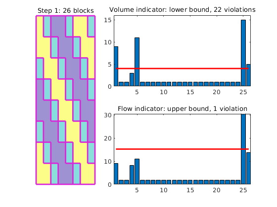
Our first example shows the four basic steps of the nonuniform coarsening algorithm proposed by Aarnes et al. [1]. The algorithm is an ad hoc approach for creating a coarse grid that distinguishes high-flow and low-flow regions, thereby trying to mimic a streamline-type grid without moving grid points. The algorithm consists of four steps:

The algorithm is a special case of a more general framework for creating coarse grids based on amalgamation of cells from a fine grid, as described by Hauge et al. [2].

mrstModule add agglom coarsegrid

Create a simple model

We consider an 8x8 Cartesian grid with an artificial flow indicator in the form of a sine-wave making an angle with the coordinate directions.

G = computeGeometry(cartGrid([8 8]));
iVel = sin(pi*(G.cells.centroids(:,1) + G.cells.centroids(:,2))/3);
iVel = iVel - min(iVel) + 1;
iVol = ones(size(iVel));
NL  = 4;
NU  = 8;

Computing normals, areas, and centroids...    Elapsed time is 0.000437 seconds.
Computing cell volumes and centroids...               Elapsed time is 0.000604 seconds.

Segement indicator

In the first step, we segment the indicator value into ten bins to distinguish the high-flow and low-flow zones.

p1 = segmentIndicator(G, iVel, 10);
plotCoarseningStep(p1, G, iVol, iVel, NL, NU, 1, 1);

SegmentIndicator: 26 blocks

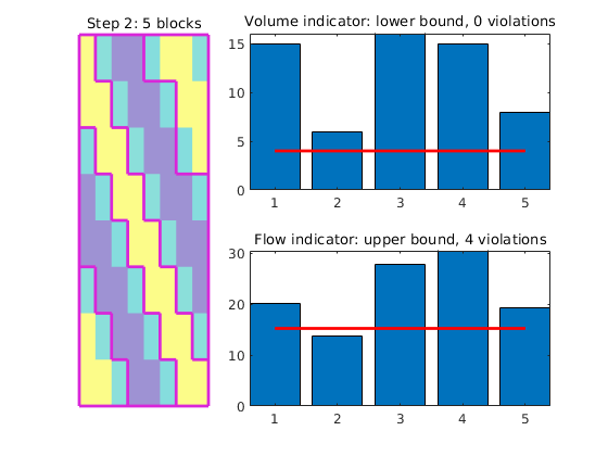
Merge blocks

The segmentation will typically create a speckle of small blocks that we do not want in our coarse grid. We therefore merge blocks that have a volume less than NL times the average cell volume with the neighboring block that has the closest iVel value.

p2 = mergeBlocks2(p1, G, iVol, iVel, NL, NU);
plotCoarseningStep(p2, G, iVol, iVel, NL, NU, 2, 1);

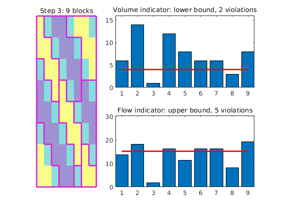
Refine blocks

In the next step we check if there are any blocks in which the iVel indicator exceeds the prescribed upper bound and if so we refine these blocks. To this end, we use a greedy algorithm that starts at one cell and grows a new block until the upper bound is exceeded. If necessary, the process is repeated.

p3 = refineGreedy(p2, G, iVel, NU);
plotCoarseningStep(p3, G, iVol, iVel, NL, NU, 3, 1);

Merge blocks

The greedy refinement may have created some small cells (typically if the blocks to be refined only slightly exceed the upper bound). We therefore perform a second merging step to get rid of blocks that have too small volume.

p4 = mergeBlocks2(p3, G, iVol, iVel, NL, NU);
plotCoarseningStep(p4, G, iVol, iVel, NL, NU, 4, 1);

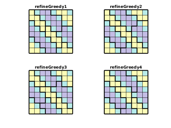
Improved refinement algorithm - part 1

The refineGreedy routine grows blocks somewhat agressively by adding rings of neighbouring cells at the time. The refineGreedy2 method only adds the neighbouring cells necessary to reach the upper limit.

p3 = refineGreedy2(p2, G, iVel, NU);
p5 = mergeBlocks2(p3, G, iVol, iVel, NL, NU);
plotCoarseningStep(p5, G, iVol, iVel, NL, NU, 4, 1);

With such small grid blocks, the algorithm does not have many choices and therefore produces a grid with two blocks that violate the upper bound. In general, it is our experience that refineGreedy2 produces better results than the original algorithm proposed by Aarnes et al.

Improved refinement algorithm - part 2

Alternatively, we can use the refineGreedy3 method which sorts the neighbouring cells in descending order by the number of faces shared with cells in the growing block. Unfortunately, the method is quite expensive and its use is not recommended for very large models.

p3 = refineGreedy3(p2, G, iVel, NU, 'nlevel',1);
p6 = mergeBlocks2(p3, G, iVol, iVel, NL, NU);
plotCoarseningStep(p6, G, iVol, iVel, NL, NU, 4, 1);

In this particular example, the resulting grid has the same number of violations as for refineGreedy2, but one of the blocks now has a stronger violation. In our experience, it is generally hard to create grids that satisfy both constraints and these should generally be seen as soft (and indicatory) bounds.

Improved refinement algorithm - part 3

As a fourth alternative, we can use the refineGreedy4 method in which the neighbouring cells are sorted in descending order in terms of the discrepancy between the flow indicator value in each neighbour cell and the growing block.

p3 = refineGreedy4(p2, G, iVel, NU, 'nlevel',1);
p7 = mergeBlocks2(p3, G, iVol, iVel, NL, NU);
plotCoarseningStep(p7, G, iVol, iVel, NL, NU, 4, 1);

In this particular example, the result is no better than for refineGreedy2. However, the method may be quite useful in some other examples.

Compare the different coarse grids

lf
p = [p4 p5 p6 p7];
for i=1:4
   subplot(2,2,i); plotCellData(G,iVel,'FaceAlpha',.3);
   outlineCoarseGrid(G,p(:,i),'Color','k'),
   title(sprintf('refineGreedy%d',i)); axis off equal
end

% <html>
% <p><font size="-1

Example 2: Constrained coarsening

Generated from agglomExample2.m

In this example we discuss how to use additional geological information to perform constrained coarsening.

mrstModule add agglom coarsegrid;

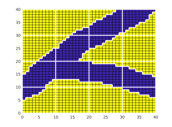
Model with two facies

As a first case, we consider 40x40 fine grid for which the image ‘facies1.png’ represents some geological object that is defined on a background. In our gridding, we will make sure that the object is represented also in the coarse model. To this end, we will partition the grid into a uniform 5x5 coarse grid and in addition preserve the edges of the object.

exdir = fullfile(mrstPath('agglom'), 'examples');
if isempty(exdir), exdir = pwd; end
imload = @(fn) ...
   flipud(double(sum(imread(fullfile(exdir, 'data', fn)), 3))) .';

f  = imload('facies1.png');
G  = computeGeometry(cartGrid(size(f)) );

ps      = compressPartition(f(:) + 1); clear f;
pu      = partitionUI(G, [4 4]);
[b,i,p] = unique([ps, pu], 'rows');
p       = processPartition(G, p);

clf,
plotCellData(G, ps);
outlineCoarseGrid(G, p, 'w');

Computing normals, areas, and centroids...    Elapsed time is 0.000247 seconds.
Computing cell volumes and centroids...               Elapsed time is 0.001619 seconds.

Let us now consider the same model, but with some ‘noise’ added outside the main object, which may or may not lead to confined blocks, i.e., blocks that are completely contained within another block. The confined blocks are marked in white color in the plot below.

f       = imload('facies2.png');
ps      = compressPartition(f(:) + 1); clear f;
[b,i,p] = unique([ps, pu], 'rows'); %#ok<*ASGLU>
p       = processPartition(G, p);
blks    = findConfinedBlocks(G, p);

clf,
plotCellData(G, ps);
outlineCoarseGrid(G, p, 'w');
for i=1:numel(blks),
   plotGrid(G,find(p==blks(i)),'FaceColor','w','edgecolor','none')
end

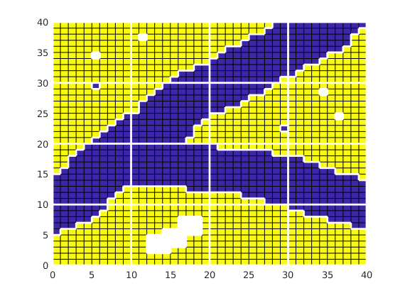
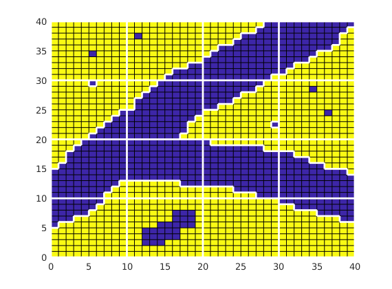
Such blocks should be detected and removed. If a block only has a single neighbour, it will have only one coarse face. This means that the block will effectively represent an obstacle to flow inside the domain in an incompressible flow simulation using net fluxes on the coarse grid.

[blks, p] = findConfinedBlocks(G, p);

clf,
plotCellData(G, ps);
outlineCoarseGrid(G, p, 'w');

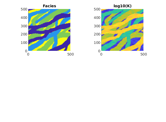
Model with four facies

As our next case, we consider a reservoir in which we have four different facies that are read from a png-image. For each facies, we generate a different lognormal permeability distribution.

f       = imload('facies3.png');
G       = computeGeometry(cartGrid(size(f), [500 500]));
k       = logNormLayers([size(f) 4],[800 50 200 1]);
[b,i,j] = unique(f); num=1:length(b);
facies  = num(j).';
K       = k( (1:numel(facies))' + (facies-1)*numel(facies));
rock.perm = K(:);
rock.poro = 0.2*ones(size(K));
clear f k;

clf,
subplot(2,2,1)
plotCellData(G, facies, 'EdgeColor', 'none')
axis equal tight, title('Facies')
subplot(2,2,2)
plotCellData(G,log10(rock.perm),'EdgeColor','none')
axis equal tight, title('log10(K)')

Computing normals, areas, and centroids...    Elapsed time is 0.001293 seconds.
Computing cell volumes and centroids...               Elapsed time is 0.011670 seconds.

Generating lognormal, layered permeability
  Layers: [ 1:1 2:2 3:3 4:4 ]
  min: 0.310571, max: 2352.56 [mD], ratio: 7574.94

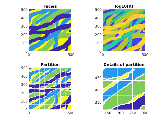
The facies distribution contain some speckles which one should be careful to get rid of as shown in the lower-right plot

u      = partitionUI(G, [8 8]);
[b,i,p] = unique([pu, facies], 'rows');
p       = processPartition(G, p);
[b,  p] = findConfinedBlocks(G, p);

subplot(2,2,3), cla
plotCellData(G,facies,'EdgeColor','none')
axis equal tight, title('Partition');
h=outlineCoarseGrid(G,p,'w'); set(h,'LineWidth',1);

subplot(2,2,4), cla
plotCellData(G,facies,'EdgeColor','none')
axis equal tight, title('Details of partition');
outlineCoarseGrid(G,p,'w'); axis([130 300 320 490])

% <html>
% <p><font size="-1

Example 3: Different Flow Indicators

Generated from agglomExample3.m

We present two examples of coarsening algorithms that fall into the general algorithmic framework described by Hauge et al [1]:

Both algorithms are applied to a 2D five-spot example with heterogeneity sampled from a lateral layer of the SPE10 model. For each algorithm, we consider three different flow indicators based on the absolute permeability, the velocity magnitude, and time-of-flight.

mrstModule add agglom coarsegrid spe10 mimetic incomp diagnostics;

Set up and solve flow problem

As our example, we consider a standard five spot with heterogeneity sampled from Model 2 of the 10th SPE Comparative Solution Project.

[G, W, rock] = getSPE10setup(25);
% Set wells to single component mode
for i = 1:numel(W)
    W(i).compi = 1;
end
rock.poro = max(rock.poro, 1e-4);
fluid = initSingleFluid('mu', 1*centi*poise, 'rho', 1014*kilogram/meter^3);
rS = initState(G, W, 0);
S  = computeMimeticIP(G, rock);
rS = incompMimetic(rS, G, S, fluid, 'wells', W);

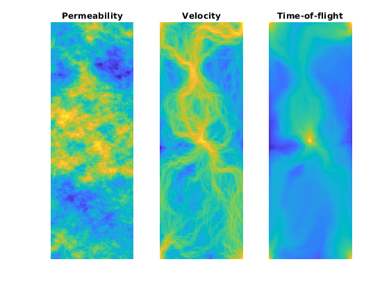
We will use the following cell-wise indicators:

For all indicators, we perform a logarithmic scaling

clf
iK = log10(rock.perm(:,1)); iK = iK - min(iK) + 1;
subplot(1,3,1); plotCellData(G,iK,'EdgeColor','none'); axis tight off
title('Permeability')

v  = faceFlux2cellVelocity(G, rS.flux); v  = sqrt(sum(v .^ 2, 2));
iV = log10(v); iV = iV - min(iV) + 1;
subplot(1,3,2); plotCellData(G,iV,'EdgeColor','none'); axis tight off;
title('Velocity')

T  = computeTimeOfFlight(rS, G, rock, 'wells', W);
Tr = computeTimeOfFlight(rS, G, rock, 'wells', W, 'reverse', true);
iT = -log10(T.*Tr); iT = iT - min(iT) + 1;
subplot(1,3,3); plotCellData(G,iT,'EdgeColor','none'); axis tight off;
title('Time-of-flight')

Uniform Refinement of High-Flow Zones

We start by a uniform 3x11 partition of the model and then add an extra 3x3 refinement in all blocks in which the block indicator exceeds the upper bound: Ib > NU*mean(Ic), where Ib is the indicator per block, Ic is the indicator per cell, and NU is a user-prescribed parameter.

p1 = partitionUI(G, [3, 11, 1]);
pK = refineUniformShape(p1, G, iK, 380, 'CartDims', [3,3,1]);
pV = refineUniformShape(p1, G, iV, 390, 'CartDims', [3,3,1]);
pT = refineUniformShape(p1, G, iT, 380, 'CartDims', [3,3,1]);

subplot(1,3,1)
outlineCoarseGrid(G, pK); title(sprintf('Permeability: %d', max(pK)))
subplot(1,3,2)
outlineCoarseGrid(G, pV); title(sprintf('Velocity: %d', max(pV)))
subplot(1,3,3)
outlineCoarseGrid(G, pT); title(sprintf('Time-of-flight: %d', max(pT)))

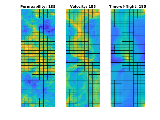
Using the two flow-based indicators iV and iT, rather than the a priori permeability indicator iK, gives grids that better adapt to the flow pattern. This is no surprise, since iK only distinguishes between zones with high permeability and low permeability, whereas the other two indicators also account for the influence of the forces that drive the flow.

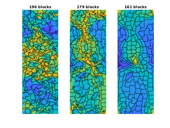
The ‘Nonuniform Coarsening’ (NUC) Algorithm

Next, we consider the nonuniform coarsening algorithm and compare the grids generated using the three flow indicators introduced above

clf
numBins  = 10;
NL       = 30;
NU       = 80;

I = [iK iV iT];
for i=1:3
   p = segmentIndicator(G, I(:,i), numBins);
   p = mergeBlocks2(p, G, rock.poro, I(:,i), NL, NU);
   p = refineGreedy2(p, G, I(:,i), NU);
   p = mergeBlocks2(p, G, rock.poro, I(:,i), NL, NU);
   subplot(1,3,i), plotCellData(G, I(:,i), 'EdgeColor', 'none')
   outlineCoarseGrid(G,p);
   axis tight off, title(sprintf('%d blocks', max(p)));
end

Warning: Some blocks still violate lower (volume) bound after merging.

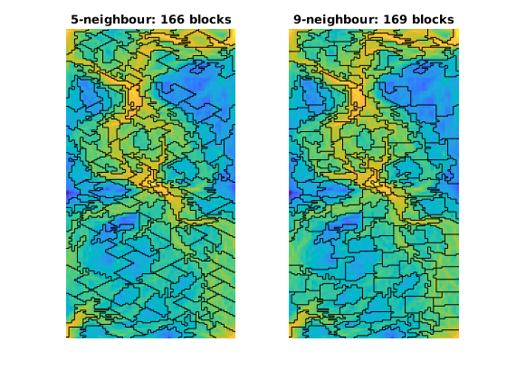
In the algorithm above, the greedy algorithm considers a 9-point neighbourhood when growing cells. In the original paper, the authors used a 5-point neighbourhood, which gives more diamond-shaped cells as shown in the figure below

clf
for i=1:2
   p = segmentIndicator(G, iV, numBins);
   p = mergeBlocks(p, G, rock.poro, iV, NL);
   p = refineGreedy2(p, G, iV, NU, 'nlevel',i);
   p = mergeBlocks(p, G, rock.poro, iV, NL);
   subplot(1,2,i), plotCellData(G, iV, 'EdgeColor', 'none')
   outlineCoarseGrid(G,p);
   axis tight off, title(sprintf('%d-neighbour: %d blocks', 2^(i+1)+1, max(p)));
end

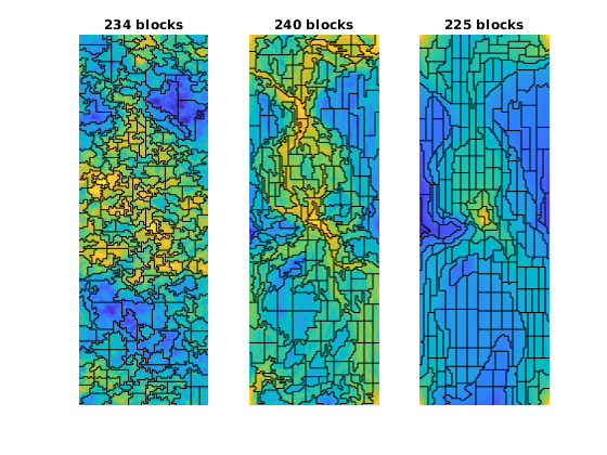
In the two previous plots, we used the greedy algorithm to refine blocks. We can, of course, also other types of refinement algorithms of each block that exceeds the upper bound on the total flow. For a Cartesian grid, the ‘refineUniform’ method performs a uniform refinement of the bounding box of each block that exceeds the upper limit.

lf
for i=1:3
   p = segmentIndicator(G, I(:,i), numBins);
   p = mergeBlocks2(p, G, rock.poro, I(:,i), NL, NU);
   p = refineUniformShape(p, G, I(:,i), NU, 'CartDims',[2,2,1]);
   p = mergeBlocks2(p, G, rock.poro, I(:,i), NL, NU);
   subplot(1,3,i), plotCellData(G, I(:,i), 'EdgeColor', 'none')
   outlineCoarseGrid(G,p);
   axis tight off, title(sprintf('%d blocks', max(p)));
end

% <html>
% <p><font size="-1

Warning: Some blocks still violate lower (volume) bound after merging.

Example 4: Nonuniform Coarsening of SPE10

Generated from agglomExample4.m

This example shows how to perform flow-based coarsening using the algorithm proposed by Aarnes et al. [1], in which the key idea is to distinguish cells in high-flow and low-flow regions. To this end, we start by the following ad-hoc algorithm:

The original algorithm consisted of the four steps above. Here, however, we repeat the last two steps a few times to obtain better grids. The resulting algorithm is a special case of a more general framework described by Hauge et al. [2]. The purpose of the example is to demonstrate the main coarsening steps for a single layer of the SPE10 model and compare the flow-adapted grid with streamlines traced from the flow field used to adapt the grid.

mrstModule add agglom coarsegrid spe10 incomp;

Set up and solve flow problem

As our example, we consider a standard five spot with heterogeneity sampled from Model 2 of the 10th SPE Comparative Solution Project, which we assume that the user has downloaded to a specific data directory using the functions supplied as part of the MRST data sets.

[G, W, rock] = getSPE10setup(25);
rock.poro    = max(rock.poro, 1e-3);
rock.perm    = rock.perm(:,1);
fluid        = initSingleFluid('mu' , 1*centi*poise     , ...
                               'rho', 1014*kilogram/meter^3);

% Solve for pressure and velocity, using no-flow boundary conditions.
rSol = initState(G, W, 0);
T    = computeTrans(G, rock);
rSol = incompTPFA(rSol, G, T, fluid, 'wells', W);

Warning: Inconsistent Number of Phases.  Using 1 Phase (=min([3, 1, 1])).

Compute indicator and set parameters used later in the algorithm

Compute a scalar, cell-wise velocity measure and use the logarithm of the velocity measure as our flow indicator

v = faceFlux2cellVelocity(G, rSol.flux);
v = sqrt(sum(v .^ 2, 2));
iVel = log10(v);
iVel = iVel - min(iVel) + 1;
NL = 10;
NU = 75;

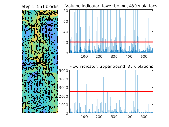
Segment indicator into bins

In the first step, we segment the indicator value into ten bins. An alternative choice could have been to set numBins = round(max(iVel)-min(iVel))

p = segmentIndicator(G, iVel, 10);
plotCoarseningStep(p, G, rock.poro, iVel, NL, NU, 1, true);

Merge small blocks

The segmentation will typically create a speckle of small blocks that we do not want in our coarse grid. Each small block is therefore merged with its neighbouring block that has the closest indicator value. Here, we use porosity as indicator when measuring which blocks to merge

p2 = mergeBlocks2(p, G, rock.poro, iVel, NL, NU);
plotCoarseningStep(p2, G, rock.poro, iVel, NL, NU, 2, true);

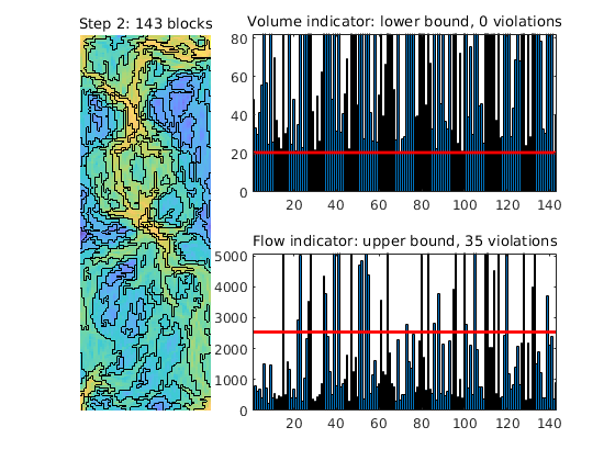
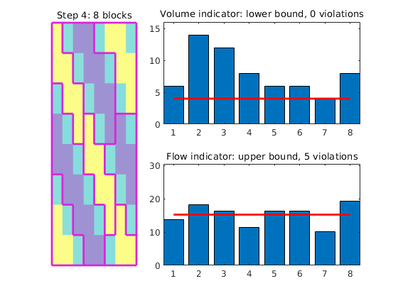
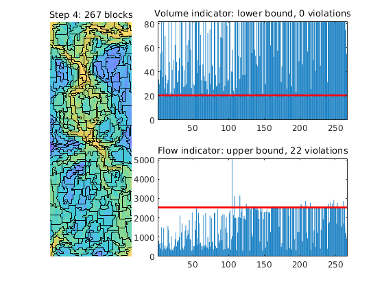
Refine blocks

Merging blocks may give new blocks through which there is too much flow. We therefore refine blocks in which the flow exceeds an upper bound.

p = refineGreedy2(p2, G, iVel, NU);
plotCoarseningStep(p, G, rock.poro, iVel, NL, NU, 3, true);

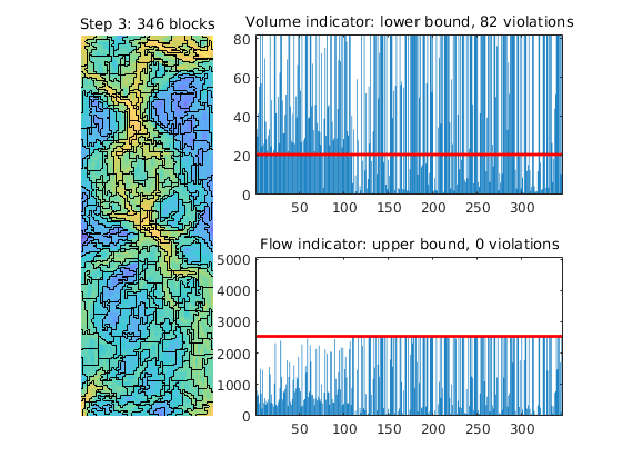
Merge small blocks

The refinement step may have created blocks that have too small volume. As a safeguard, we merge these

p = mergeBlocks2(p, G, rock.poro, iVel, NL, NU);
[b, p] = findConfinedBlocks(G, p);
plotCoarseningStep(p, G, rock.poro, iVel, NL, NU, 4, true);

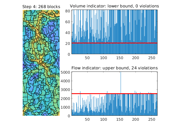
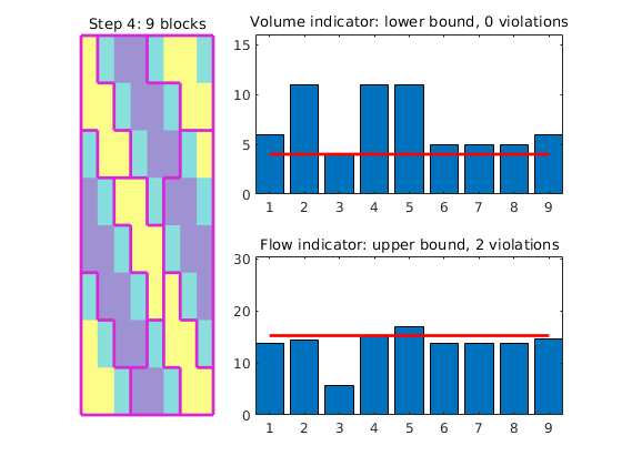
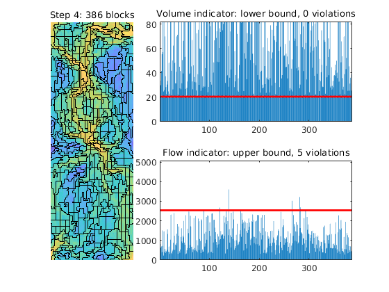
Repeat refinement and merging

p = refineGreedy2(p, G, iVel, NU);
p =  mergeBlocks2(p, G, rock.poro, iVel, NL, NU);
plotCoarseningStep(p, G, rock.poro, iVel, NL, NU, 4, true);

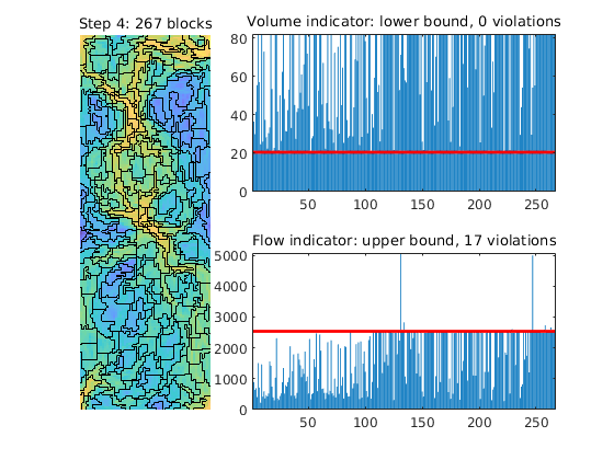
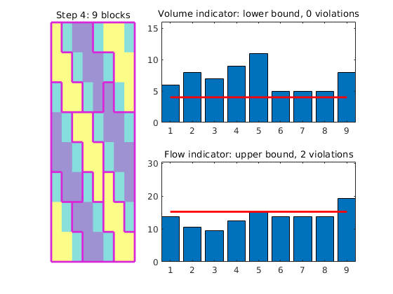
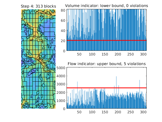
p = refineGreedy2(p, G, iVel, NU);
p = mergeBlocks2(p, G, rock.poro, iVel, NL, NU);
plotCoarseningStep(p, G, rock.poro, iVel, NL, NU, 4, true);

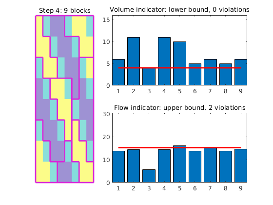
Other refinement algorithms

The refineGreedy routine grows blocks somewhat agressively by adding rings of neighbouring cells at the time. The results are typically worse than for refineGreedy2

p = refineGreedy(p2, G, iVel, NU);
[b, p] = findConfinedBlocks(G, p);
p = mergeBlocks2(p, G, rock.poro, iVel, NL, NU);
plotCoarseningStep(p, G, rock.poro, iVel, NL, NU, 4, 1);

Better results may be obtained if we use the refineGreedy3 method in which the neighbouring cells are sorted in descending order in terms of the number of faces shared with cells in the growing block. Unfortunately, the method is quite expensive and its use is not recommended for large models.

p = refineGreedy3(p2, G, iVel, NU, 'nlevel',2);
[b, p] = findConfinedBlocks(G, p); %#ok<*ASGLU>
p = mergeBlocks2(p, G, rock.poro, iVel, NL, NU);
plotCoarseningStep(p, G, rock.poro, iVel, NL, NU, 4, 1);

Alternatively, we can perform a Cartesian refinement of each block, which leads to a higher number of blocks.

pC = refineUniformShape(p2, G, iVel, NU,'cartDims', [2 2 1]);
pC = mergeBlocks2(pC, G, rock.poro, iVel, NL, NU);
[b, p] = findConfinedBlocks(G, p);
plotCoarseningStep(pC, G, rock.poro, iVel, NL, NU, 4, 1);

Or, we can perform a refinement in which we try to impose a fixed default partition in all parts that exceed the upper bound. And if this is not sufficient, we further subdivide the remaining violating blocks rectangularly.

pf = partitionUI(G, [6 22 1]);
pC = refineUniformShape(p2, G, iVel, NU,'fixPart', pf, 'CartDims',[2 1 1]);
pC = mergeBlocks2(pC, G, rock.poro, iVel, NL, NU);
[b, p] = findConfinedBlocks(G, p);
plotCoarseningStep(pC, G, rock.poro, iVel, NL, NU, 4, 1);

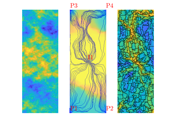
Compare with streamlines

To show how the NUC grid adapts to the flow field, we plot permeability field, pressure field with streamlines, and flow-adapted grid. As we can observe from the figure, the flow-adapted grid aligns neatly with the high-flow and low-flow regions

lf,
subplot(1,3,1)
plotCellData(G,log10(rock.perm),'EdgeColor','none'); axis tight off

subplot(1,3,2)
mrstModule add streamlines
plotCellData(G,rSol.pressure,'FaceAlpha',.5,'EdgeColor','none');
nx = G.cartDims(1);
cells = [...
   (-nx/6:nx/6) + W(5).cells - 4*nx, (-nx/6:nx/6) + W(5).cells + 4*nx, ...
   (0:nx/10) + W(1).cells + 4*nx, (-nx/10:0)+W(2).cells + 4*nx, ...
   (0:nx/10) + W(3).cells - 4*nx, (-nx/10:0)+W(4).cells - 4*nx, ...
   ];
h = streamline(pollock(G, rSol, cells')); set(h,'Color','b');
rSol.flux = -rSol.flux;
h = streamline(pollock(G, rSol, cells')); set(h,'Color','b');
rSol.flux = -rSol.flux;
plotWell(G,W); axis tight off

subplot(1,3,3)
plotCellData(G,iVel,'EdgeColor','none')
outlineCoarseGrid(G, p); axis tight off

% <html>
% <p><font size="-1

Example 5: Hybrid Grids

Generated from agglomExample5.m

In this example we discuss how to combine flow adaption with a regular partition, which can be done in several ways.

mrstModule add agglom coarsegrid spe10 incomp diagnostics;

Set up and solve flow problem

As our example, we consider a standard five spot with heterogeneity sampled from Model 2 of the 10th SPE Comparative Solution Project.

[G, W, rock] = getSPE10setup(25);
rock.poro = max(rock.poro, 1e-4);
fluid = initSingleFluid('mu', 1*centi*poise, 'rho', 1014*kilogram/meter^3);
rS = initState(G, W, 0);
rS = incompTPFA(rS, G, computeTrans(G, rock), fluid, 'wells', W);

Compute flow indicators based on velocity and time-of-flight

iK = log10(rock.perm(:,1)); iK = iK - min(iK) + 1;
v  = faceFlux2cellVelocity(G, rS.flux); v  = sqrt(sum(v .^ 2, 2));
iV = log10(v); iV = iV - min(iV) + 1;
T  = computeTimeOfFlight(rS, G, rock, 'wells', W);
Tr = computeTimeOfFlight(rS, G, rock, 'wells', W, 'reverse', true);
iT = -log10(T.*Tr); iT = iT - min(iT) + 1;

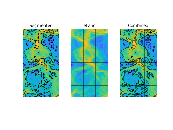
Combine a Uniform and a Flow-Based Partition

As our first example of a hybrid grid we will combine a uniform partition with a segmentation based on velocities. The two partitions are generated independently and then merged using the builtin ‘unique’ function (which may be expensive for very large grids). Afterwards, we process the partition to check for disconnected blocks that need to be split.

clf
targs = {'FontSize',10,'FontWeight','normal'};
p1 = segmentIndicator(G, iV, 4);
pS = partitionUI(G, [3,6,1]);
[b, i, p] = unique([pS, p1], 'rows'); %#ok<*ASGLU>
p  = processPartition(G, p);

subplot(1,3,1), title('Segmented',targs{:})
plotCellData(G,iV,'EdgeColor','none')
outlineCoarseGrid(G,p1); axis equal tight off

subplot(1,3,2), title('Static',targs{:})
plotCellData(G,iV,'EdgeColor','none')
outlineCoarseGrid(G,pS); axis equal tight off

subplot(1,3,3), title('Combined',targs{:})
plotCellData(G,iV,'EdgeColor','none')
outlineCoarseGrid(G,p); axis equal tight off

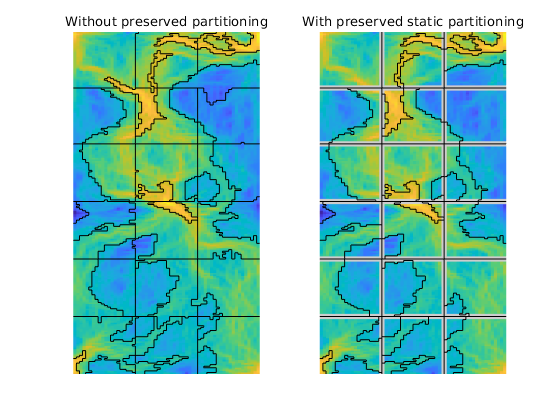
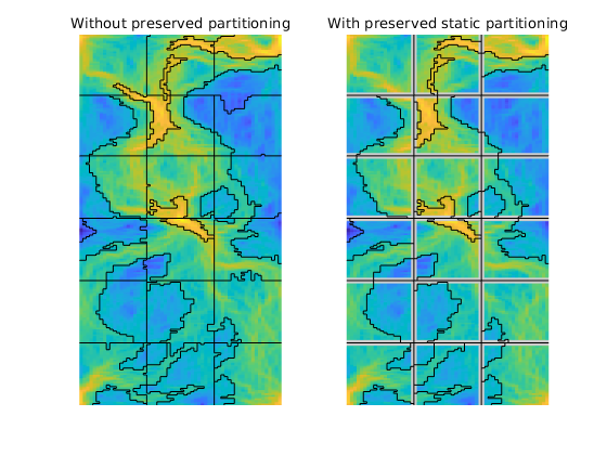
If the a priori partitioning should be preserved throughout the coarsening, we specify it in the option 'static_partition' in the call to mergeBlocks. Then the interfaces in this partitioning will not be crossed.

p1 = mergeBlocks(p, G, rock.poro, iV, 30);
p2 = mergeBlocks(p, G, rock.poro, iV, 30, 'static_partition', pS);

We then plot the result to confirm that the uniform partition is preserved in p2.

clf;
subplot(1,2,1);
plotCellData(G, iV, 'EdgeColor', 'none');
h1 = outlineCoarseGrid(G, p1); axis equal tight off;
title('Without preserved partitioning',targs{:});

subplot(1,2,2);
plotCellData(G, iV, 'EdgeColor', 'none');
outlineCoarseGrid(G, pS,'EdgeColor',[.8 .8 .8],'LineWidth',4);
h2 = outlineCoarseGrid(G, p2); axis equal tight off;
title('With preserved static partitioning',targs{:});

Both partitions would typically be used as input to further refinement and merging steps. If not, we should get grid of all blocks that are confined within another block.

delete([h1, h2])
subplot(1,2,1),
[blks, p1] = findConfinedBlocks(G,p1);
outlineCoarseGrid(G, p1);

subplot(1,2,2),
[blks, p2] = findConfinedBlocks(G,p2);
outlineCoarseGrid(G, p2);

Compare Uniform, NUC, and Hybrid Grids

In the next example, we compare three different algorithms

The parameters in the methods are chose so that the number of coarse blocks should be somewhat lower than the 528 blocks in a 12 x 44 uniform Cartesian partition.

clf
cgDims = [12 44 1];
NB = prod(bsxfun(@rdivide, G.cartDims, cgDims));
NL = .5*NB;
NU = 1.1*NB;

pu = partitionUI(G, cgDims);
pt = segmentIndicator(G, iT, 12);
p = mergeBlocks(pt, G, rock.poro, iT, NL);
p = refineGreedy3(p, G, iT, NU);
p = mergeBlocks(p, G, rock.poro, iT, NL);
[b, p] = findConfinedBlocks(G, p);
subplot(1,4,1)
plotCellData(G, iT, 'EdgeColor', 'none'), outlineCoarseGrid(G,p);
axis tight off, title(sprintf('TOF:\n%d blocks', max(p)),targs{:});

p = mergeBlocks(pt, G, rock.poro, iT, NL);
p = refineUniformShape(p, G, iT, NU, 'fixPart', pu);
p = mergeBlocks(p, G, rock.poro, iT, 0.75*NL);
[b, p] = findConfinedBlocks(G, p);
subplot(1,4,2)
plotCellData(G, iT, 'EdgeColor', 'none'), outlineCoarseGrid(G,p);
axis tight off, title(sprintf('Hybrid TOF:\n%d blocks', max(p)),targs{:});

pv = segmentIndicator(G, iV, 10);
p = mergeBlocks(pv, G, rock.poro, iT, NL);
p = refineGreedy3(p, G, iT, NU);
p = mergeBlocks(p, G, rock.poro, iT, NL);
[b, p] = findConfinedBlocks(G, p);
subplot(1,4,3)
plotCellData(G, iV, 'EdgeColor', 'none'), outlineCoarseGrid(G,p);
axis tight off, title(sprintf('Vel:\n%d blocks', max(p)),targs{:});

ps = partitionUI(G, [6 22 1]);
[b,j,p]  = unique([pv, ps], 'rows');
p  = processPartition(G, p);
p = mergeBlocks(p, G, rock.poro, iV, NL);
p = refineGreedy3(p, G, iV, NU);
p = mergeBlocks(p, G, rock.poro, iV, NL, 'static_partition', ps);
[b, p] = findConfinedBlocks(G, p);
subplot(1,4,4)
plotCellData(G, iV, 'EdgeColor', 'none'), outlineCoarseGrid(G,p);
axis tight off, title(sprintf('Hybrid vel:\n%d blocks', max(p)),targs{:});

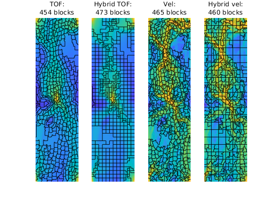
Comparing the two time-of-flight grids, we see that the hybrid approach ensures that the blocks are more regular in regions of low flow. Comparing the hybrid time-of-flight and the hybrid velocity grid, we see that the latter has regular coarse blocks in all zones of low flow because of the static 6x22 partition.

<html>
% <p><font size="-1

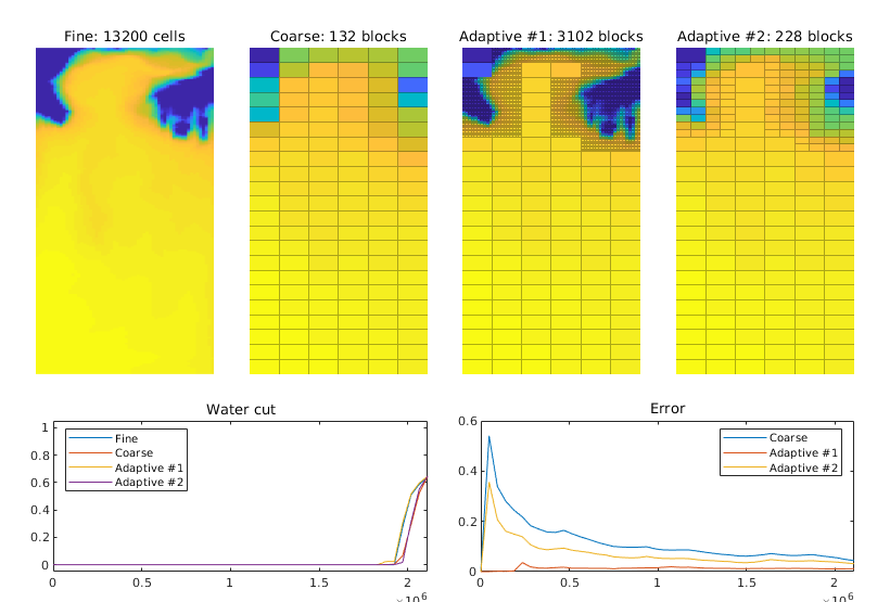
Example 6: Adaptive Refinement of Grid

Generated from agglomExample6.m

In this example, we show how to make grids that dynamically adapt to an advancing saturation front. To this end, we consider a quarter five-spot with heterogeneity sampled from on layer of the SPE10 data set. We will compare the solution transport on four different grids (using pressure solutions computed on the fine grid):

Where to refine is predicted by comparing the solution at the previous time step with a coarse-grid estimation of the next time step. Refinement can then be imposed either cell-wise for all cells where the discrepancy is larger than satTol or blockwise in all blocks in which the discrepancy is larger than satTol. For the block-wise refinement, we also refine block neighbors across interfaces with net flux below fluxTol to reduce coarse-scale smearing.

mrstModule add agglom coarsegrid spe10 diagnostics incomp mimetic;

Parameters controlling case setup

layer = 20;          % which layer from the SPE10 model
adaptBlocks = true;  % refine all cells within a marked block
useCart = true;      % use Cartesian coarse grid
satTol  = .02;       % refine if |s-s.old|>satTol
fluxTol = 1e-2;      % refine on both sides when net flux is below fluxTol

Initialize model problem and compute initial solution

Create grid structure, rock structure, and source structure, and initalise a fluid object. Note the viscosities. For simpler flow-pattern we use a quarter five-spot source/sink configuration, instead of the five-spot well configuration.

gravity off

[G, W, rock] = getSPE10setup(25); clear W %#ok<ASGLU>
rock.poro    = max(rock.poro, 1e-3);
fluid        = initSimpleFluid('mu' , [   1,  .2]*centi*poise     , ...
                               'rho', [1014, 859]*kilogram/meter^3, ...
                               'n'  , [   2,   2]);
src  = addSource([], [1 G.cells.num], [1000 -1000]./day(), 'sat', [1, 0]);

Simulation parameters

param.nPres = 9;   % Pressure steps
param.nSub  = 5;   % Transport steps per pressure step
pv          = poreVolume(G, rock);
T           = .9 * sum(pv) / sum(src.rate(src.rate > 0)); % PVI -> time
DT          = T / (param.nPres * param.nSub);
[NL,NU]     = deal(50, 100);
[NLF,NUF]   = deal(10, 25);

Compute initial fine-grid solution

rf = initState(G, [], 0, 0);
S  = computeMimeticIP(G, rock);
rf = incompMimetic(rf, G, S, fluid, 'src', src);

Create basic coarse grid and supporting data structures

We generate a quite coarse grid used for estimatating which regions to refine adaptiv around the advancing saturation front. This is the same grid throughout the whole simulation process.

iTOF = log10(1 ./ ( ...
   computeTimeOfFlight(rf, G, rock, 'src', src) .* ...
   computeTimeOfFlight(rf, G, rock, 'src', src, 'reverse', true)));
iTOF  = iTOF - min(iTOF) + 1;

% Make static partitions and coarse grid
pS = partitionUI(G, [12 44 1]);
if useCart,
   p = partitionUI(G, [6 22 1]);
else
   p = segmentIndicator(G, iTOF, 2*round(max(iTOF) - min(iTOF)) ); %#ok<UNRCH>
   p = mergeBlocks2(p, G, pv./G.cells.volumes, iTOF, NL, NU);
   p = refineGreedy2(p, G, iTOF, NU);
   p = mergeBlocks2(p, G, pv./G.cells.volumes, iTOF, NL, NU);
   [b, bi, pS] = unique([pS, p], 'rows');
end
[blks, p] = findConfinedBlocks(G,p);
CG  = generateCoarseGrid(G, p);
pvC = accumarray(CG.partition,pv);

% Adding extra coarse grid fields to not stop in twophaseJacobian, getFlux
CG.cells.volumes = accumarray(CG.partition, G.cells.volumes);
CG.nodes.coords  = zeros(CG.cells.num, 3);
CG.faces.normals = zeros(CG.faces.num, 3);

% To find coarse net fluxes on coarse interfaces from fine fluxes
[nsubC, subC] = subFaces(G, CG);
[sgnC, cfC] = signOfFineFacesOnCoarseFaces(G, CG, nsubC, subC);

% Coarse rock and source structure
rockC.poro = accumarray(CG.partition, pv)./CG.cells.volumes;
srcC  = convertSource2Coarse(CG, src);

% Initially, all coarse grids are the same
aG1 = CG;
aG2 = CG;

Set correct fluxes for the state vectors

rf - fine grid rc - coarse grid, rc contains fine-grid and rcC coarse-grid quantities ra1 - adaptive #1, ra1 contains fine-grid and ra1C coarse-grid quantities ra2 - adaptive #2, ra2 contains fine-grid and ra2C coarse-grid quantities

rcC.flux       = accumarray(cfC, sgnC.*rf.flux(subC), [CG.faces.num,1]);
rcC.s          = coarse_sat(rf.s, CG.partition, pv, CG.cells.num);
[rc, ra1, ra2] = deal(rf);
[ra1C, ra2C]   = deal(rcC);
[ra1C.cflux, ra2C.cflux] = deal(rcC.flux);

Time loop

0 = get(gcf, 'OuterPosition');
clf, set(gcf, 'OuterPosition', [p0(1:2), 820, 640]);
wc  = zeros(param.nPres*param.nSub+1, 4); wc(2:end,:) = NaN;
err = zeros(param.nPres*param.nSub+1, 3); err(2:end,:) = NaN;
T   = 0:DT:T;
mytitle =@(x) title(x, 'FontSize',10,'FontWeight','normal');
for i = 1:param.nPres,
   for j = 1:param.nSub,

      % Fine and coarse solution
      rf   = implicitTransport(rf, G, DT, rock, fluid, 'src', src);

      rcC  = implicitTransport(rcC, CG, DT, rockC, fluid, 'src', srcC);
      rc.s = rcC.s(CG.partition);

      % Adaptive grid with local fine-grid resolution
      % Predict new saturation on coarse grid
      est.flux = ra1C.cflux;
      est.s    = coarse_sat(ra1.s, CG.partition, pv, CG.cells.num);
      est      = implicitTransport(est, CG, DT, rockC, fluid, 'src', srcC);
      est.s    = est.s(CG.partition);

      % Determine which cells to refine
      if adaptBlocks,
         disc  = accumarray(CG.partition, abs(est.s - ra1.s).*pv)./ pvC;
         blks = [false; disc>satTol];
         N = double(CG.faces.neighbors( ...
            abs(ra1C.cflux) < fluxTol*max(ra1C.cflux),:)+1);
         blks(N(any(blks(N),2),:)) = true;
         blks = blks(2:end);
         cells = blks(CG.partition);
      else
         cells = abs(est.s - ra1.s)>satTol; %#ok<UNRCH>
      end

      % Update partition and create new grid
      pn        = CG.partition;
      pn(cells) = CG.cells.num + (1:sum(cells));
      pn        = compressPartition(pn);
      pn        = processPartition(G, pn);
      aG1       = generateCoarseGrid(G, pn);

       % Additional fields in the coarse grid
      aG1.cells.volumes = accumarray(aG1.partition, G.cells.volumes);
      aG1.nodes.coords  = zeros(aG1.cells.num, 3);
      aG1.faces.normals = zeros(aG1.faces.num, 3);

      % Updating structures
      [nsub,sub] = subFaces(G, aG1);
      [sgn,  cf] = signOfFineFacesOnCoarseFaces(G, aG1, nsub, sub);
      pvb        = accumarray(aG1.partition, pv);
      rockb.poro = pvb ./ aG1.cells.volumes;
      srcb       = convertSource2Coarse(aG1, src);
      ra1C.flux  = accumarray(cf, sgn .* ra1.flux(sub), [aG1.faces.num,1]);
      ra1C.s     = accumarray(aG1.partition, ra1.s.*pv) ./ pvb;

      % Transport simulation
      ra1C = implicitTransport(ra1C, aG1, DT, rockb, fluid, 'src', srcb);
      ra1.s = ra1C.s(aG1.partition);

      % Adaptive grid with local refinement (from pS)
      % Predict new saturation on coarse grid
      est.flux = ra2C.cflux;
      est.s    = coarse_sat(ra2.s, CG.partition, pv, CG.cells.num);
      est      = implicitTransport(est, CG, DT, rockC, fluid, 'src', srcC);
      est.s    = est.s(CG.partition);

      % Determine which cells to refine
      if adaptBlocks,
         disc  = accumarray(CG.partition, abs(est.s - ra2.s).*pv)./ pvC;
         blks = [false; disc>satTol];
         N = double(CG.faces.neighbors(...
            abs(ra2C.cflux) < fluxTol*max(ra2C.cflux),:)+1);
         blks(N(any(blks(N),2),:)) = true;
         blks = blks(2:end);
         cells = blks(CG.partition);
      else
         cells = abs(est.s - ra2.s)>satTol; %#ok<UNRCH>
      end

      % Update partition and create new coarse grid
      pn        = CG.partition;
      ps        = compressPartition(pS(cells));
      pn(cells) = max(pn) + ps;
      pn        = compressPartition(pn);
      pn        = processPartition(G, pn);
      aG2       = generateCoarseGrid(G, pn);

      % Additional fields in the coarse grid
      aG2.cells.volumes = accumarray(aG2.partition, G.cells.volumes);
      aG2.nodes.coords  = zeros(aG2.cells.num, 3);
      aG2.faces.normals = zeros(aG2.faces.num, 3);

      % Updating structures
      [nsub,sub] = subFaces(G, aG2);
      [sgn,  cf] = signOfFineFacesOnCoarseFaces(G, aG2, nsub, sub);
      pvb        = accumarray(aG2.partition, pv);
      rockb.poro = pvb ./ aG2.cells.volumes;
      srcb       = convertSource2Coarse(aG2, src);
      ra2C.flux  = accumarray(cf, sgn .* ra2.flux(sub), [aG2.faces.num,1]);
      ra2C.s     = accumarray(aG2.partition, ra2.s.*pv) ./ pvb;

      % Transport simulation on  aG2
      ra2C   = implicitTransport(ra2C, aG2, DT, rockb, fluid,  'src', srcb);
      ra2.s  = ra2C.s(aG2.partition);

      % Plotting of saturations
      clf
      axes('position',[.04 .35 .2 .6])
      plotCellData(G, rf.s, 'EdgeColor', 'none'), axis equal tight off
      mytitle(sprintf('Fine: %d cells', G.cells.num));

      axes('position',[.28 .35 .2 .6])
      plotCellData(G, rc.s, 'EdgeColor', 'none'), axis equal tight off
      outlineCoarseGrid(G, CG.partition, 'EdgeColor', 'w', 'EdgeAlpha', 0.3);
      mytitle(sprintf('Coarse: %d blocks', CG.cells.num));

      axes('position',[.52 .35 .2 .6])
      plotCellData(G, ra1.s, 'EdgeColor', 'none'), axis equal tight off
      outlineCoarseGrid(G, aG1.partition, 'EdgeColor', 'w', 'EdgeAlpha', 0.3);
      mytitle(sprintf('Adaptive #1: %d blocks', aG1.cells.num))

      axes('position',[.76 .35 .2 .6])
      plotCellData(G, ra2.s, 'EdgeColor', 'none'), axis equal tight off
      outlineCoarseGrid(G, aG2.partition, 'EdgeColor', 'w', 'EdgeAlpha', 0.3);
      mytitle(sprintf('Adaptive #2: %d blocks', aG2.cells.num));


      % Plot error curves and water cut
      ind = (i-1)*param.nSub + j+1;
      axes('position',[.06 .05 .42 .25])
      wc(ind,:) = [ rf.s(G.cells.num), rc.s(G.cells.num), ...
                    ra1.s(G.cells.num), ra2.s(G.cells.num) ];
      plot(T, wc),
      legend('Fine','Coarse', 'Adaptive #1', 'Adaptive #2', ...
             'Location', 'NorthWest');
      axis([T(1) T(end) -.05 1.05]), mytitle('Water cut')

      axes('position',[.54 .05 .42 .25])
      err(ind,:) = [sum(abs(rc.s - rf.s).*pv), ...
                    sum(abs(ra1.s - rf.s).*pv), ...
                    sum(abs(ra2.s - rf.s).*pv)]./sum(rf.s .* pv);
      plot(T, err),
      legend('Coarse', 'Adaptive #1', 'Adaptive #2', ...
             'Location', 'NorthEast');
      set(gca,'XLim',[T(1) T(end)]), mytitle('Error')

      drawnow
   end

   % Update fine-grid pressure
   rf  = incompMimetic(rf, G, S, fluid, 'src', src);

   % Update fine-grid pressure for CG, convert fluxes to coarse structure
   rc = incompMimetic(rc, G, S, fluid, 'src', src);
   rcC.flux = accumarray(cfC, sgnC .* rc.flux(subC), [CG.faces.num, 1]);

   % Update fine-grid pressure for aG1 and aG2
   ra1 = incompMimetic(ra1, G, S, fluid, 'src', src);
   ra2 = incompMimetic(ra2, G, S, fluid, 'src', src);

   % Compute net flux along underlying coarse grid
   ra1C.cflux = accumarray(cfC, sgnC .* ra1.flux(subC), [CG.faces.num, 1]);
   ra2C.cflux = accumarray(cfC, sgnC .* ra2.flux(subC), [CG.faces.num, 1]);
   % Fluxes for the adaptive coarse grid will be updated after the grid has
   % been generated in the main loop.
end

% <html>
% <p><font size="-1