`streamlines`: Compute streamlines¶

This module implements Pollock’s method for streamline-tracing on structured grids. Streamlines are very useful for visualizing flow patterns and understanding connectivity in a reservoir. Note that this model does not presently implement a streamline solver for the transport problem.

Contents¶

STREAMLINES Support for streamline-based methods

Files: pollock - Trace streamlines in logically Cartesian grid using Pollock approximation.

pollock(G, state, varargin)¶

Trace streamlines in logically Cartesian grid using Pollock approximation.

Synopsis:

[S,T,C] = pollock(G, state)
[S,T,C] = pollock(G, state, startpos)
[S,T,C] = pollock(G, state, 'pn', pv, ...)
[S,T,C] = pollock(G, state, startpos, 'pn', pv, ...)

Parameters:	G – Cartesian or logically Cartesian grid. state – State structure with field ‘flux’.

OPTIONAL PARAMETER

positions - Matrix of size (N, 1) or (N, d+1), where d is the dimension

of the grid, used to indicate where the streamlines should start.

If the size is (N, 1), positions contains the cell indices in which streamlines should start. Each streamline is started in the the local coordinate (0.5, 0.5, …). To be precise, this is the mean of the corner points, not the centroid of the cell.

If the size is (N, d+1), the first column contains cell indices, and the d next columns contain the local coordinates at which to start streamlines.

Keyword Arguments:

substeps – Number of substeps in each cell, to improve visual quality. Default 5.
maxsteps – Maximal number of points in a streamline. Default 1000.
reverse – Reverse velocity field before tracing. Default false.
pvol – Pore-volume vector. One positive scalar for each active cell in the grid G. Makes the physical interpretation of time-of-flight appropriate for non-uniform porosity fields.
isoutflow – Cell-wise boolean indicator which indicates if a streamline should terminate upon reaching that cell. Defaults to false(G.cells.num, 1) and is useful in the presence of many weak source terms (which do not lead to inflow or outflow over all faces for a given source term).
blocksize – Internal parameter indicating how many streamlines are processed simultaneously. Larger values give faster processing, at a higher memory cost. Default: 1000.

Returns:

S – Cell array of individual streamlines suitable for calls like streamline(pollock(…)) and streamtube(pollock(…)).
T – Time-of-flight of coordinate.
C – Cell number of streamline segment, i.e, line segment between two streamline coordinates.

Example:

S = pollock(G, x);
% pad with nan's
S = reshape([S, repmat({[nan, nan]}, [numel(S),1])]',[], 1);
S = vertcat(S{:});
plot(S(:,1), S(:,2), 'r-');

streamline(pollock(G, x, 'pvol', poreVolume(G, rock)));

Examples¶

Streamlines for a 2D Quater Five-Spot Well Pattern¶

Generated from testPollock2D.m

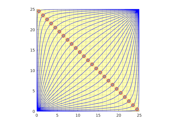
The quarter five-spot problem is one of the cases that are most widely used to test numerical methods. The setup consist of an injector and a producer located in diagonally oposite corners, with no-flow conditions along the model perimeter. This gives a symmetric flow pattern with high flow along the diagonal and stagnant points at the corners with no wells.

mrstModule add mimetic incomp streamlines

Construct model and compute flow field¶

G = cartGrid([25,25]);
G = computeGeometry(G);

rock = makeRock(G, 10*milli*darcy, 0.3);

fluid = initSimpleFluid('mu',  [1, 1]*centi*poise', ...
                        'rho', [1000, 1000]*kilogram/meter^3, ...
                        'n',   [2, 2]);

T = computeTrans(G, rock);
src = addSource([], [1, G.cells.num], [1.1, -1.1]);

x = initResSol(G, 0, 0);
x = incompTPFA(x, G, T, fluid, 'src', src);

Trace streamlines¶

Pick start points on the diagonal orthogonal to the well-pair direction and trace streamlines forward and backward from these points. This will ensure maximal accuracy in the near-well regions where the streamlines are converging.

clf
h = plotGrid(G, 'facea', 0.3, 'edgea',0.1);
hold on;
cells = (G.cartDims(1):G.cartDims(1)-1:prod(G.cartDims)-1)';
streamline(pollock(G, x, cells));
x.flux = -x.flux;
streamline(pollock(G, x, cells, 'substeps', 1));
plot(G.cells.centroids(cells,1), G.cells.centroids(cells,2), ...
    'or','MarkerSize',8,'MarkerFaceColor',[.6 .6 .6]);
axis equal tight
hold off

Copyright notice¶

<html>
% <p><font size="-1

Streamlines for a 3D Quater Five-Spot Well Pattern¶

Generated from testPollock3D.m

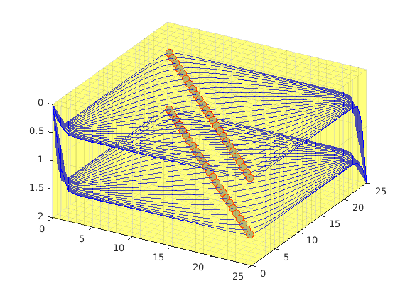
The setup consist of a vertical injector and a vertical producer located in the southwest and northeast corners, respectively. This gives a symmetric areal flow pattern with high flow along the diagonal and stagnant points at the southeast and northwest corners. The setup is almost the same as in the 2D test, except that we now use a consistent discretization from the mimetic module.

mrstModule add mimetic incomp streamlines

Set up model¶

G = cartGrid([25,25,2]);
G = computeGeometry(G);
rock = makeRock(G, 10*milli*darcy, 0.3);

fluid = initSimpleFluid('mu',  [1, 1]*centi*poise', ...
                        'rho', [1000, 1000]*kilogram/meter^3, ...
                        'n',   [2, 2]);

IP = computeMimeticIP(G, rock);
src = addSource([], [1, G.cells.num], [1, -1]);
x = initResSol(G, 0, 0);
x = incompMimetic(x, G, IP, fluid, 'src', src);

Trace streamline¶

clf
h = plotGrid(G, 'facea', 0.3, 'edgea',0.1);
hold on;
cells = (G.cartDims(1):G.cartDims(1)-1:prod(G.cartDims)/2-1)';
cells = [cells; cells+prod(G.cartDims)/2];
streamline(pollock(G, x, cells));
x.flux = -x.flux;
streamline(pollock(G, x, cells, 'substeps', 1));
plot3(G.cells.centroids(cells,1), G.cells.centroids(cells,2), ...
     G.cells.centroids(cells,3), ...
    'or','MarkerSize',8,'MarkerFaceColor',[.6 .6 .6]);
hold off
axis tight, view(30,40)

Copyright notice¶

<html>
% <p><font size="-1

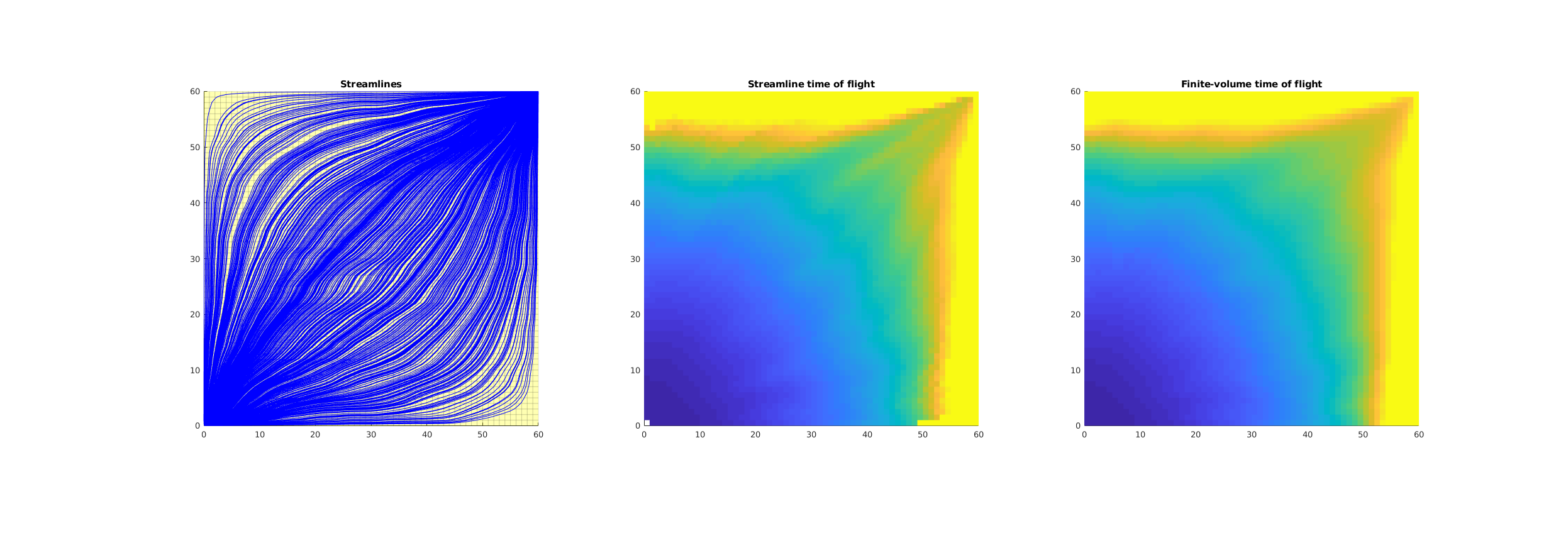
Compare Time-of-Flight Computed by Steamlines and by Finite-Volumes¶

Generated from testPollockTOF.m

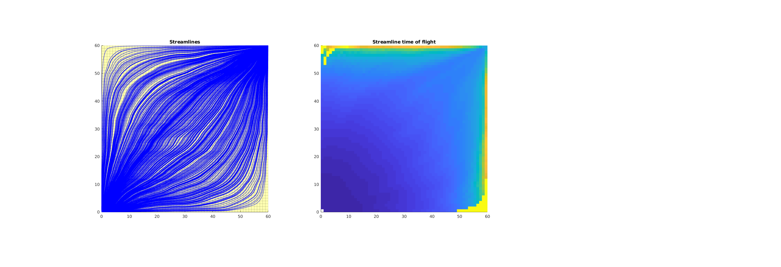
MRST offers two ways of computing time-of-flight for Cartesian grids:

Pollock’s method gives pointwise values of high accuracy for Cartesian grids, but this method has not yet been implemented for general unstructured grids. The finite-volume method computes time-of-flight in a volume-averaged sense, and will hence not have high pointwise accuracy, but can readily be applied to any type of valid MRST grid.

mrstModule add mimetic incomp diagnostics streamlines

Setup model and solve flow problem¶

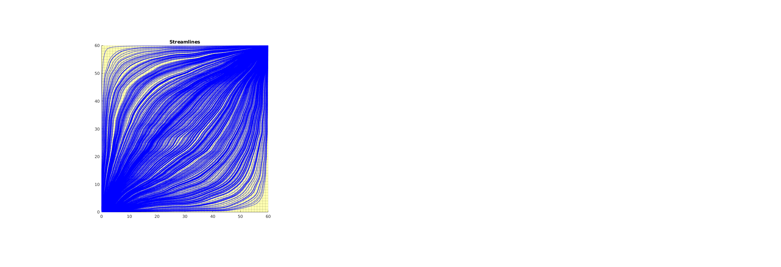
We consider a 60x60 grid with a quarter five-spot well pattern. The petrophysical quantities can either be uniform, or sampled from a Gaussian distribution. Pollock’s method is not yet implemented for non-unit porosity values, but this minor deficiency can be circumvented by appropriate postprocessing and scaling of cell increments

G = cartGrid([60,60]);
G = computeGeometry(G);

%perm = 10*milli*darcy;
perm = convertFrom(logNormLayers([G.cartDims, 1], 1), milli*darcy);
poro = 1;
rock = makeRock(G, perm, poro);

fluid = initSimpleFluid('mu',  [   1,    1]*centi*poise, ...
                        'rho', [1000, 1000]*kilogram/meter^3, ...
                        'n',   [   2,    2]);

IP = computeMimeticIP(G, rock);
src = addSource([], [1, G.cells.num], [1.1, -1.1], 'sat', [1.0 0.0;1.0,0.0]);

x = initResSol(G, 0, 0);
x = incompMimetic(x, G, IP, fluid, 'src', src);

Trace and plot streamlines¶

numStreamlines = 500;
clf
scrsz = get(0,'ScreenSize');
set(gcf,'Position',[0 scrsz(4)-scrsz(3)/3 scrsz(3) scrsz(3)/3]);
subplot(1,3,1);
title('Streamlines');
h = plotGrid(G, 'facea', 0.3, 'edgea',0.1);
axis equal tight;
pos = [ones(numStreamlines,1), rand(numStreamlines,2)];
timer=tic;
[xyz,t,c] = pollock(G, x, pos, 'substeps', 1, 'maxsteps',10000);
thetime=toc(timer);
dispif(true, 'Traced %d steps in %d streamlines in %g second\n', ...
   sum(cellfun(@numel, t)), numStreamlines, thetime);
streamline(xyz);

Traced 60004 steps in 500 streamlines in 0.107208 second

Extract time-of-flight¶

subplot(1,3,2);
title('Streamline time of flight')

% add time of flight along streamlines
ct = cellfun(@cumsum, t, 'uniformoutput', false);

% rearrange to plain double arrays
t  = vertcat(t{:});
i= (t ~= inf);
t  = t(i);
ct = vertcat(ct{:}); ct = ct(i);
c  = vertcat(c{:});  c  = c(i);

% Compute weigthed average of time of flight in each cell that has been
% crossed by one or more streamlines,
%
%    tof_i = sum(t_ij*ct_ij; j) / sum(t_ij; j)
%
% where t_ij is the time-of-flight diff through cell i of streamline j

tof = accumarray(c, ct.*t, [G.cells.num, 1], [], inf)./...
   accumarray(c, t,     [G.cells.num, 1], [], 1);


plotCellData(G, tof, 'EdgeColor','none');
axis equal tight;

Compute time-of-flight using diagnostics tools¶

subplot(1,3,3);
title('Finite-volume time of flight')
fdTOF = computeTimeOfFlight(x, G, rock, 'src', src);
plotCellData(G, fdTOF,'EdgeColor','none');
axis equal tight;

% Use fdTOF for caxis scalling as this does not change randomly.
subplot(1,3,2), caxis([0,fdTOF(src.cell(end))])
subplot(1,3,3), caxis([0,fdTOF(src.cell(end))])

Copyright notice¶

<html>
% <p><font size="-1

streamlines: Compute streamlines¶

Examples¶

Streamlines for a 2D Quater Five-Spot Well Pattern¶

Construct model and compute flow field¶

Trace streamlines¶

Copyright notice¶

Streamlines for a 3D Quater Five-Spot Well Pattern¶

Set up model¶

Trace streamline¶

Copyright notice¶

Compare Time-of-Flight Computed by Steamlines and by Finite-Volumes¶

Setup model and solve flow problem¶

Trace and plot streamlines¶

Extract time-of-flight¶

Compute time-of-flight using diagnostics tools¶

Copyright notice¶

`streamlines`: Compute streamlines¶