steady-state Steady-state upscaling of functions
Functionality for upscaling relative permeabilities based on a steady-state assumption. This includes general steady state, as well as capillary and viscous-dominated limits. The functionality is demonstrated through a few tutorial examples.
See the ‘upscaling’ module for functionality for single-phase upscaling.
-
Contents¶ STEADY-STATE
- Files
- GridBlock - Base class for upscaling a single block OnePhaseUpscaler - One phase upscaling TwoPhaseTwoStepUpscaler - Two phase upscaling TwoPhaseUpscaler - Two phase upscaling Upscaler - Base class for upscaling classes
-
class
GridBlock(G, rock, varargin)¶ Base class for upscaling a single block
-
static
findSideFaces(G)¶ Given a grid, find the side faces on each side in each direction. NOTE: This method assumed a high regularity of the grid, and may fail for more complex grids.
-
G= None¶ Grid structure for the block. May be periodic.
-
areas= None¶ Side areas
-
bcp= None¶ Periodic boundary conditions. Empty if periodic is false.
-
faces= None¶ Side faces
-
fluid= None¶ Fluid structure for the block. May be empty.
-
lengths= None¶ Vector of characteristic length for each dimension.
-
periodic= None¶ Boolean. True if block is periodic and false otherwise.
-
periodicDims= None¶ Dimensions which are made periodic. Defaulted to all.
-
pv= None¶ Pore volume
-
rock= None¶ Rock structure for the block. Used for upscaling.
-
rockorg= None¶ Original rock structure.
-
verbose= None¶ deck for the block only. May be empty.
-
static
-
class
OnePhaseUpscaler(G, rock, varargin)¶ One phase upscaling
-
class
TwoPhaseTwoStepUpscaler(G, rock, fluid, varargin)¶ Two phase upscaling
-
createBlock(upscaler, cells)¶ Create grid, rock and fluid for the sub block represented by the given cells.
-
upscaleBlock(upscaler, block)¶ Because the slizes will contain only a single cell in a direction, periodic boundaries cannot be applied without using some tricks
-
-
class
TwoPhaseUpscaler(G, rock, fluid, varargin)¶ Two phase upscaling
-
createBlock(upscaler, cells)¶ Create grid, rock and fluid for the sub block represented by the given cells.
-
RelpermAbsMethod= None¶ Abs-perm upscaling used in relperm upscaling
-
RelpermMethod= None¶ Relperm upscaling method
-
nrelperm= None¶ Whether to include gravity in pcOW upscaling
-
relpermdims= None¶ Dimensions to upscale relperm in
-
savesat= None¶ Save saturation distributions
-
-
class
Upscaler(G, rock, varargin)¶ Base class for upscaling classes
-
createBlock(upscaler, cells)¶ Create grid, rock and fluid for the sub block represented by the given cells.
-
static
createBlockDeck(deck, cells)¶ Create a sub deck for the block based on the given cells NOTE: This function assumes a Cartesian grid.
-
upscale(upscaler)¶ Given some partition, we loop over the coarse blocks in the grid and upscale each of them in turn.
-
deck= None¶ Index map for the blocks. Equal index means equal block.
-
verbose= None¶ Estimate time remaining
-
-
Contents¶ UTILS
- Files
- addFracFlowInvADIFluid - Add a fluid function for computing the inverse of the water fractional addPcOWInvADIFluid - Add a fluid function for computing the inverse of the capillary pressure. cartBlockMap - Find identical coarse blocks in a partition of a Cartesian grid. This createBlockFluid - Extracting the fluid for the current coarse cell only. createFracFlowTablesFromDeck - Undocumented Utility Function initADIFluidOW - Make a structure representing an oil-water fluid. This is might be a initADIFluidOWPolymer - Make a structure representing a three-component fluid (water, oil, makePeriodicCartesianGrid - Undocumented Utility Function simulateToSteadyStateADI - Run simulation to a steady state solution is found using fully implicit struct2args - Converts a structure to a cell array with both fieldnames and values,
-
addFracFlowInvADIFluid(fluid, deck, varargin)¶ Add a fluid function for computing the inverse of the water fractional flow curve. This may be called later by using
sW = fluid.fracFlowInv(ff)The input deck must have the properties SWOF, PVTW and PVCDO.
Fractional flow = (krW/muW) / ( (krW/muW) + (krO/muO) )
-
addPcOWInvADIFluid(fluid, deck, varargin)¶ Add a fluid function for computing the inverse of the capillary pressure. This may be called later by using
sW = fluid.pcOWinv(pc)The input deck must have the property SWOF.
-
cartBlockMap(G, rock, partition, varargin)¶ Find identical coarse blocks in a partition of a Cartesian grid. This function returns a map, which split all coarse cells into max(map) number of groups. All coarse cell j with map(j)==i are in group i, and are considered identical, i.e. they share the exact same properties and are equivalent wrt. upscaling.
-
createBlockFluid(fluid, cells)¶ Extracting the fluid for the current coarse cell only.
-
createFracFlowTablesFromDeck(deck)¶ Undocumented Utility Function
-
initADIFluidOW(varargin)¶ Make a structure representing an oil-water fluid. This is might be a helpful function for examples and testing.
See initADIFluidOWPolymer for more information.
-
initADIFluidOWPolymer(varargin)¶ Make a structure representing a three-component fluid (water, oil, polymer) and their properties (relative permeabilities, densities, viscosities, etc.). This is might be a helpful function for examples and testing.
Synopsis:
fluid = initADIFluidOWPolymer()
fluid = initADIFluidOWPolymer('pn1', 'pv1', ...)
Parameters: - 'pn'/pv – List of ‘key’/value pairs defining optional parameters. The supported options are as follows:
- regnum – Fluid index. The grid is divided into N regions, where each region has different fluid properties. This parameter is a vector of length G.cells.num, such that cell i belongs to fluid area reginx(i). If empty, entire grid has the same properties.
- FLUID PROPERTY PARAMETERS:
‘pn’/pv - List of ‘key’/value pairs defining optional parameters. Each property value can be given in of one of the following four forms:
Constant in entire grid. Input form: P=k, where k is a scalar. The property value will be set to k in all cells.
Constant in each region. Input form: P=v, where v is a vector of size N-by-1, where N is the number of regions, The property value will be set to v(i) in all cells of region i.
Piecewise linear function, same function in entire domain. Input form: P=T, where T is matrix of size M-by-2. The linear function is defined by the M points (xi,yi), where xi=T(i,1) and yi=T(i,2)).
Piecewise linear function, different function in each region. Input form: P={T1,…,TN}, where Ti is matrix of size M-by-2, defining the linear function for region i. N is the number of regions.
Piecewise linear function of two variables (x,v), same function in entire domain. Input form: P=T, where T is structure with the following fields:
T.key - The v values. T.pos - Maps vi values to the data field, such that
T.data(T.pos(i):(T.pos(i+1)-1), :)
gives the x and y values corresponding to vi=T.key(i).
- T.data - A matrix of size M-by-2, where xj=T.data(j,1) and
yj=T.data(j,2).
Note that if a property value is empty, the property is not added to the fluid structure.
The supported properties are as follows:
Water/Oil properties: muW - Water viscosity (Pa*s), function of water pressure muO - Oil viscosity (Pa*s), function of oil pressure rhoW - Water density (kg/m^3) rhoO - Oil density (kg/m^3) BW - Water formation volume factor (FVF), function of water
pressureBO - Oil formation volume factor (FVF), function of oil pressure krW - Water relative permeability, function of water saturation krO - Oil relative permeability, function of oil saturation pvMultR - Pressure-dependent pore volume multiplier, function of oil
pressure.Polymer properties: cmax - Maximum polymer concentration (kg/m^3) ads - Adsorption isoterm (kg/kg), function of polymer
concentration (kg/m^3)adsMax - Maximum allowed adsorbed polymer (kg/kg) muWMult - Water viscosity multiplier (kg/m^3), function of polymer
- concentration (kg/m^3). muWMult is defined such that
- muM(c) = muW.*muWMult(c)
where muM(c) is the viscosity of a fully mixed polymer solution.
dps - Dead pore space rrf - Residual resistance factor rhoR - Mass density of the rock formation (kg/m^3) mixPar - Todd-Longstaff mixing parameter omega
Returns: fluid – ADI fluid structure with the given properties.
-
makePeriodicCartesianGrid(G)¶ Undocumented Utility Function
-
simulateToSteadyStateADI(G, rock, fluid, sW0, varargin)¶ Run simulation to a steady state solution is found using fully implicit adi solver.
Synopsis:
state           = simulateToSteadyStateADI(G, rock, fluid, state0, ...
                      'pn', pv, ...)
[state, report] = simulateToSteadyStateADI(...)
Parameters: - state0 – initial state
- G – grid structure
- rock – rock structure
- fluid – fluid structure
- OPTIONAL PARAMETERS
- ‘pn’/pv - List of ‘key’/value pairs defining optional parameters.
- The supported options are as follows:
bc - fixed boundary conditions Gp - periodic grid structure bcp - periodic boundary conditions dtInit - initial timestep dtIncFac - timestep multiplyer for increasing timestep dtMax - maximum timestep allowed dtIncTolSat - tolerence factor on the change in saturation for when
to increase timestepabsTolPres - absolute pressure tolerence absTolSat - absolute saturation tolerence absTolFlux - absolute flux tolerence absTolPoly - absolute polymer tolerence nIterMax - maximum number of iterations
Returns: - state – steady state solution
- meta – (OPTIONAL) meta data structure
-
struct2args(s, varargin)¶ Converts a structure to a cell array with both fieldnames and values, which may be used as arguments to an MRST function.
- SYNOPSIS:
- c = struct2cellWithNames(s)
- PARAMETERS:
- s - Single structure.
- OPTIONAL PARAMETERS:
- ‘pn’/pv - List of ‘key’/value pairs defining optional parameters. The
- supported options are:
include - Only include the field names given in this cell array. remove - Remove the field names given in this cell array.
Note: remove will be ignored if include is given.- RETURNS:
- c - Cell array of the form {‘field1’, value1, ‘field2’, value2, …. }
- where the ‘field’ strings are the fieldnames of s. The following entry in c is the corresponding value of that field in s.
- COMMENTS:
If s contains N fields, then c will contain 2*N elements.
The retured cell array c may be used to create a comma seperated list by calling c{:}.
See also STRUCT, CELL, STRUCT2CELL.
-
Contents¶ AD
- Files
- equationsOilWater_BCP - Get linearized problem for oil/water system with black oil-style getFluxAndPropsOil_BO_BCP - Undocumented Utility Function getFluxAndPropsWater_BO_BCP - Undocumented Utility Function TwoPhaseOilWaterModel_BCP - Two phase oil/water system without dissolution
-
class
TwoPhaseOilWaterModel_BCP(G, rock, fluid, varargin)¶ Two phase oil/water system without dissolution
-
TwoPhaseOilWaterModel_BCP(G, rock, fluid, varargin)¶ model = model@TwoPhaseOilWaterModel(G, rock, fluid, varargin{:});
-
-
equationsOilWater_BCP(state0, state, model, dt, drivingForces, varargin)¶ Get linearized problem for oil/water system with black oil-style properties
-
getFluxAndPropsOil_BO_BCP(model, p, p_prop, sO, krO, T, gdz, rs, isSat, bcp)¶ Undocumented Utility Function
-
getFluxAndPropsWater_BO_BCP(model, pO, p_prop, sW, krW, T, gdz, bcp)¶ Undocumented Utility Function
-
Contents¶ COARSEGRID
- Files
- addNodeDataToCoarseGrid - Add node data to upscaled grid CG createUpscaledFluid - Creates an upscaled fluid from given data.
-
addNodeDataToCoarseGrid(CG)¶ Add node data to upscaled grid CG
Assumptions: - Each face has four nodes. - Each face is a rectangle - Each face is normal to one of the main directions
NOTE: NOT SURE ABOUT THE ORDERING OF THE NODES WITHIN EACH FACE. THIS MAY BE A PROBLEM IF GRID IS PASSED ON TO E.G. computeGeometry, WHICH ASSUMES A SPEECIAL ORDERING OF THE NODES.
-
createUpscaledFluid(f, updata, partition)¶ Creates an upscaled fluid from given data.
-
Contents¶ UPSCALING
- Files
- getCapVisDist - Upscale two-way oil-water distribution pcVsUpscaledSwGravityBinary - Create fine scale capillary pressure pc as a function of upscaled sW. upAbsPerm - Undocumented Utility Function upAbsPermAvg - Power averaging of of the absolute permeability upAbsPermPres - Undocumented Utility Function upFracFlowOW - Upscale fractional flow curves. upPcOW - Upscale capillary pressure curves. upPolyAds - Upscale polymer adsorption isotherm using a simple average. upPolyRk - Undocumented Utility Function upPoro - Upscale porosity of the block by pore volume averaging upRelPerm - Upscaling of relative permeability upRelPermEPS - Upscaling of relperm curves by end-point scaling (EPS) upRelPermPV - Undocumented Utility Function upscaleTransNew - Calculate upscaled transmissibilities for a coarse model upWells - Upscale wells
-
getCapVisDist(block, pcVal, varargin)¶ Upscale two-way oil-water distribution
-
pcVsUpscaledSwGravityBinary(G, rock, fluid, varargin)¶ Create fine scale capillary pressure pc as a function of upscaled sW.
Parameters: - G – Grid structure.
- rock – Rock structure.
- fluid – Fluid structure. Must have a field called ‘pcOWInv’.
Returns: - pcFun – function handle to a function taking upscaled sW as input, and returning the corresponding capillary pressure.
- swUMin – minimum upscaled water saturation
- swUMax – maximum upscaled water saturation
-
upAbsPerm(block, updata, varargin)¶ Undocumented Utility Function
-
upAbsPermAvg(block, updata, varargin)¶ Power averaging of of the absolute permeability
-
upAbsPermPres(block, updata, varargin)¶ Undocumented Utility Function
-
upFracFlowOW(block, updata, varargin)¶ Upscale fractional flow curves.
It is assumed that all fractional flow curves are monotone.
-
upPcOW(block, updata, varargin)¶ Upscale capillary pressure curves.
It is assumed that all capillary pressure curves are monotone.
The upscaling is done my looping over different values of the capillery pressure. For each value, this value is set in all cells, and then the capillary pressure function is inverted to find the saturation distribution. The saturation is then upscaled, and we have a pair of saturation/pcOW.
-
upPolyAds(block, updata, varargin)¶ Upscale polymer adsorption isotherm using a simple average.
The adsorption isotherm which is a function of the local polymer solution concentration.
-
upPolyRk(block, updata, method, varargin)¶ Undocumented Utility Function
-
upPoro(block, updata)¶ Upscale porosity of the block by pore volume averaging
-
upRelPerm(block, updata, method, varargin)¶ Upscaling of relative permeability
-
upRelPermEPS(block, updata, method, varargin)¶ Upscaling of relperm curves by end-point scaling (EPS)
-
upRelPermPV(block, updata, method, varargin)¶ Undocumented Utility Function
-
upWells(CG, rock, W, varargin)¶ Upscale wells
-
upscaleTransNew(cg, T_fine, varargin)¶ Calculate upscaled transmissibilities for a coarse model
Synopsis:
[HT_cg, T_cg, cgwells, upscaled] = upscaleTrans(cg, T_fine)
[HT_cg, T_cg, cgwells, upscaled] = ...
    upscaleTrans(cg, T_fine, 'pn1', pv1, ...)
Parameters: - cg – coarse grid using the new-coarsegrid module structure
- T_fine – transmissibility on fine grid
- 'pn'/pv –
- List of ‘key’/value pairs for supplying optional parameters.
- The supported options are
- Verbose – Whether or not to display informational
- messages throughout the computational process. Logical. Default value: Verbose = false (don’t display any informational messages).
- bc_method choise of global boundary condition method.
- Valid choises is ‘bc_simple’ (default), ‘bc’ need option ‘bc’ ‘wells_simple’, need option ‘wells’ with one well configuration and give an upscaled well cgwells as output ‘wells’ need ‘wells as’ cellarray and do not upscale wells
- match_method how to match to the set of global boundary
- conditions options are
‘max_flux’lsq_flux’
- fix_trans ‘true/false’ set negative and zero
- transmissibility to lowest positive found
- opt_trans_alg use optimization of trans base valide values
- ’none’,’local’,’global’
- opt_trans_method method for optimizing trans ‘linear_simple’,’
- ’convecs_simple’
Returns: - HT_cg – One-sided, upscaled transmissibilities
- T_cg – Upscaled interface transmissibilities
- cgwells – Coarse grid well with upscaled well indices
- upscaled – Detailed infomation from the upscaling procedure. For testing purposes.
See also
coarsegrid module,
grid_structure
-
interp1q_mex(varargin)¶ Undocumented Utility Function
Examples
Periodic Boundary Conditions for AD code
Generated from periodicBoundaryExample.m
We demonstrate the use of periodic boundary conditions. This is implemented as part of this module only using ‘hacked’ versions of the ad-blackoil models. Note that there is a limitation in the implementation of the periodic boundary conditions, such each dimension must have at least two cells.
mrstModule add ad-blackoil ad-core ad-props upscaling steady-state
Setup example
We set up a very simple incompressible model with periodic boundary conditions.
% Create grid
G = cartGrid([50, 2, 2], [100, 10, 10]*meter);
G = computeGeometry(G);

% Make the grid periodic
[Gp, bcp] = makePeriodicCartesianGrid(G);

% Homogenous rock properties
rock = struct('perm', 1000*ones(G.cells.num, 1)*milli*darcy, ...
              'poro', ones(G.cells.num, 1));

% Default fluid with unit values
fluid = initSimpleADIFluid();

% The fluid is incompressible. We have to tell the solver explicitly that
% this is the case to avoid a singular Jacobian matrix.
fluid.isIncomp = true;

% Set up model. We use a hacked version of the TwoPhaseOilWaterModel which
% allows for periodic boundary conditions.
model = TwoPhaseOilWaterModel_BCP(Gp, rock, fluid);

% Initial state with an oil slug in the middle of the domain
ijk = gridLogicalIndices(Gp);
inx = ijk{1} >= 25 & ijk{1} <= 40;
state0 = initResSol(Gp, 50*barsa, [1, 0]);
state0.s(inx,1) = 0;
state0.s(inx,2) = 1;
state0.wellSol = initWellSolAD([], model, state0);

% Set pressure drop over boundary
bcp.value(bcp.tags == 1) = -400*barsa;
Run simulation
solver = NonLinearSolver();
dT = 50*day;
n = 35;
states = cell(n+1, 1);
states{1} = state0;
for i = 1:n
    state = standaloneSolveAD(states{i}, model, dT, 'bcp', bcp);
    states{i+1} = state;
end
Solving timestep 1/1:         -> 50 Days
*** Simulation complete. Solved 1 control steps in 298 Milliseconds ***
Solving timestep 1/1:         -> 50 Days
*** Simulation complete. Solved 1 control steps in 118 Milliseconds ***
Solving timestep 1/1:         -> 50 Days
*** Simulation complete. Solved 1 control steps in 30 Milliseconds ***
Solving timestep 1/1:         -> 50 Days
*** Simulation complete. Solved 1 control steps in 28 Milliseconds ***
...
Plot animation of the solution
Observe how the oil slug exits the boundary on the right and enters on the left as the grid is periodic.
inx = ijk{2}==1 & ijk{3}==1;
x = G.cells.centroids(inx,1);
figure(1); clf;
for i=1:n
    cla;
    plot(x, states{i}.s(inx,2), 'r');
    axis([0 max(x) 0 1]);
    drawnow;
    pause(0.10); if i==1, pause(1); end
end
Layered Model Polymer Upscaling Example
Generated from LayeredPolymerExample.m
This example demonstrates polymer upscaling of a simple layered model. The upscaling of polymer is described in [1], and this example is identical the first example in therein. There exists an analytical solution to the upscaling, and so this example serves as a verification. Step through the code blocks of the script. References: [1] Hilden, Lie and Xavier Raynaud - “Steady State Upscaling of Polymer Flooding”, ECMOR XIV - 14th European conference on the mathematics of oil recovery, 2014.
Add MRST modules
% Add this module
mrstModule add steady-state

% We rely on the following MRST modules
mrstModule add incomp upscaling ad-props ad-core ad-blackoil
Open a new figure and make it wide
fh = figure;
set(fh, 'Name', 'Layered Model Example', 'NumberTitle', 'off');
op = get(fh, 'OuterPosition');
set(fh, 'OuterPosition', op.*[1 1 2.4 1]);

Create grid
% Grid structure
G = cartGrid([3 3 3]);
G = computeGeometry(G);
ijk = gridLogicalIndices(G);

% Set middel layer is rock #2, while top and bottom layers are rock #1
regnum = ones(G.cells.num,1);
regnum(ijk{3}==2) = 2;

% Rock
K = [100 0.1].*milli*darcy;
clear rock
rock.perm = K(1).*ones(G.cells.num,1);
rock.perm(regnum==2) = K(2);
rock.poro = 0.1.*ones(G.cells.num,1);

% Fluid with different relperms in the two regions
fprop = getExampleFluidProps(rock, 'satnum', regnum, ...
    'swir', 0, 'sor', 0, 'krWmax', 1, 'krn', [2.5 1.5], ...
    'nsat', 50, 'polymer', true);
fprop.pcOW = [];
fprop.rhoO = 1000;
fprop.rhoW = 1000;
fprop.muO = 1*centi*poise;
fprop.muW = 1*centi*poise;

% Polymer properties
fprop.ads = {[ [ 0; 0.3; 1.5; 2.6;  4].*kilogram/meter^3, ...
               [ 0;  15;  27;  30; 30].*(milli*gram)/(kilo*gram) ], ...
             [ [ 0; 0.3; 1.5; 2.7;  4].*kilogram/meter^3, ...
               [ 0;  10;  20;  25; 25].*(milli*gram)/(kilo*gram) ] };
fprop.adsMax = [30; 25].*(milli*gram)/(kilo*gram);
fprop.muWMult = [ [ 0;  1;  3;  4].*kilogram/meter^3, ...
                  [ 1;  3; 37; 40] ];
fprop.rrf = [3.2; 1.4];

Rkorg = cell(1,2);
for r=1:2
    Rkorg{r} = [fprop.ads{r}(:,1), ...
        1 + (fprop.rrf(r)-1).*( fprop.ads{r}(:,2)./fprop.adsMax(r) ) ];
end

fluid = initADIFluidOWPolymer(fprop);
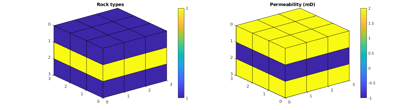
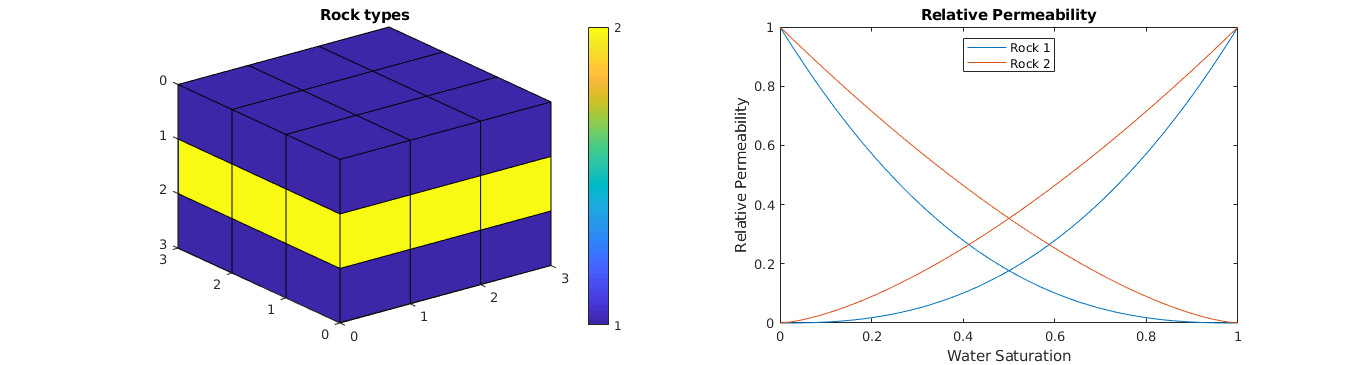
Plot the grid
% Plot the regions
clf; subplot(1,2,1);
plotCellData(G, regnum);
view(3); axis tight; cbh = colorbar; title('Rock types');
set(cbh, 'YTick', [1 2]);

% Plot the permeability
subplot(1,2,2);
plotCellData(G, log10(convertTo(rock.perm(:,1), milli*darcy)));
view(3); axis tight; colorbar; title('Permeability (mD)');
Plot relative permeabilities
% Plot the regions
clf; subplot(1,2,1);
plotCellData(G, regnum);
view(3); axis tight; cbh = colorbar; title('Rock types');
set(cbh, 'YTick', [1 2]);

% Plot the relative permeability
subplot(1,2,2); cla; hold on;
colors = lines(2); lh = nan(2,1);
for r=1:2
    lh(r) = plot(fprop.krW{r}(:,1), fprop.krW{r}(:,2), ...
                'Color', colors(r,:) );
            plot(1-fprop.krO{r}(:,1), fprop.krO{r}(:,2), ...
                'Color', colors(r,:) );
end
box on; axis([0 1 0 1]); title('Relative Permeability');
legend(lh,{'Rock 1','Rock 2'},'Location','North');
xlabel('Water Saturation'); ylabel('Relative Permeability');
Plot polymer properties
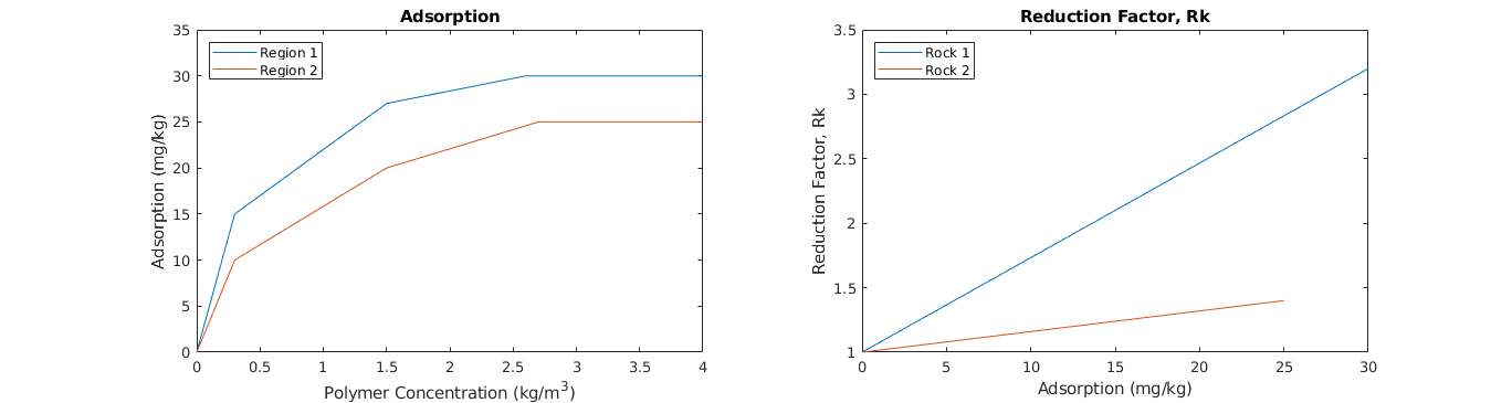
% Adsorption
clf; subplot(1,2,1); hold on;
colors = lines(2); lh = nan(2,1);
for r=1:2
    lh(r) = plot(fprop.ads{r}(:,1), fprop.ads{r}(:,2).*(10^6), ...
                'Color', colors(r,:) );
end
box on; title('Adsorption'); axis([0 4 0 35]);
legend(lh,{'Region 1','Region 2'},'Location','NorthWest');
xlabel('Polymer Concentration (kg/m^3)'); ylabel('Adsorption (mg/kg)');

% Reduction Factor
subplot(1,2,2); hold on;
lh = nan(2,1);
for r=1:2
    lh(r) = plot(fprop.ads{r}(:,2).*(10^6), Rkorg{r}(:,2));
end
legend(lh,{'Rock 1','Rock 2'},'Location','NorthWest');
box on; title('Reduction Factor, Rk'); axis([0 30 1 3.5]);
xlabel('Adsorption (mg/kg)'); ylabel('Reduction Factor, Rk');
Upscale absperm
% Create grid block
block = GridBlock(G, rock, 'fluid', fluid, 'periodic', true);

% Upscale porosity
updata = upPoro(block);

% Upscale absolute permeability
updata = upAbsPerm(block, updata);
Compute analytical solution
This example has an analytical solution for the absolute permeability, relative permeability and the reduction factor, as described in [1]. This allows us to compare the numerical flow-based solution with the analytical solution as a verification.
updataA = LayeredExactUpscaling(K, fprop.krW, fprop.krO, Rkorg);
Compare absolute permeability upscaling
To verify that the absolute permeability is correctly upscaled, we compare the numerically computed values with the analytical solution.
KA = updataA.perm./(milli*darcy);
KN = updata.perm./(milli*darcy);
fprintf('\nUpscaled absolute permeability\n');
fprintf('Analytical: [%1.2f, %1.2f, %1.2f]\n', KA(1), KA(2), KA(3));
fprintf('Numerical:  [%1.2f, %1.2f, %1.2f]\n', KN(1), KN(2), KN(3));
fprintf('Rel.diff.:  %1.2e\n\n', norm( (KA-KN)./KA ) );
Upscaled absolute permeability
Analytical: [66.70, 66.70, 0.30]
Numerical:  [66.70, 66.70, 0.30]
Rel.diff.:  6.35e-13
Upscale relative permeability
We upscale the relative permeability using flow-based steady-state upscaling with periodic boundary conditions (periodicity is determined by the creation of the block structure above). The flow-based upscaling is rather time-consuming, as a two-phase flow simulation is run for each upscaled saturation value and each dimension. As the model is symmetric in x-y, we only upscale in the x- and z-direction to save computation. But still, e.g. requesting 15 upscaled values, the number of flow simulations amounts to 13*2=26 . We do not need to run the endpoints, as one of the phases is then immobile and the solution is known a priori.
% Upscale relative permeability
updata = upRelPerm(block, updata, 'flow', 'nsat', 15, 'dims', [1 3], ...
    'verbose', true);
Starting relperm upscaling
   #      sW   Time(s)
  1/15   0.00   0.03
  2/15   0.07   1.13
  3/15   0.14   0.48
  4/15   0.21   0.50
  5/15   0.29   0.39
...
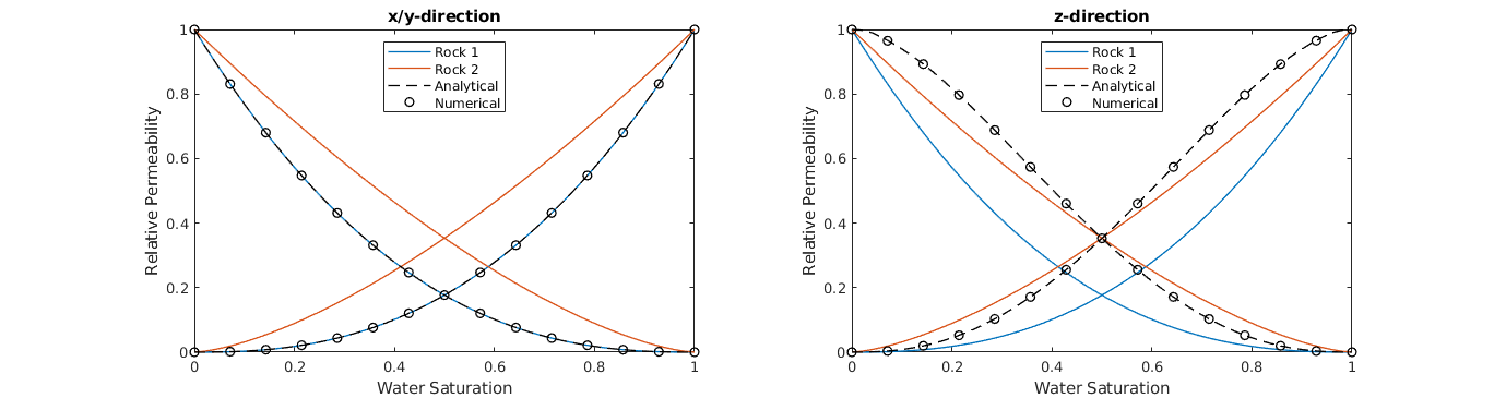
Plot upscaled relative permeability
The upscaling of the relative permeabilities are also computed analytically, and we compare the analytical solution with the numerically flow-based upscaled curves. This plot is equivalent to Figure 2 in [1].
clf;
lw = 1;
colors = lines(numel(updata.krW));
lh = nan(4,1);
dims = [1 3];

% Plot both x- and z-direction. y is equal to x.
for i=1:2
    d = dims(i);
    subplot(1,2,i); hold on;

    % Plot original curves first
    for r=1:2
        lh(r) = plot(fprop.krW{r}(:,1), fprop.krW{r}(:,2), ...
                    'Color', colors(r,:), 'LineWidth', lw );
                plot(1-fprop.krO{r}(:,1), fprop.krO{r}(:,2), ...
                    'Color', colors(r,:), 'LineWidth', lw );
    end

    % Plot analytical upscaling
    lh(3) = plot(updataA.krW{d}(:,1), updataA.krW{d}(:,2), 'k--', ...
        'LineWidth', lw );
    plot(updataA.krO{d}(:,1), updataA.krO{d}(:,2), 'k--', ...
        'LineWidth', lw );

    % Plot numerical upscaling. Note that the second dimension is z, so we
    % use index i instead of d.
    lh(4) = plot(updata.krW{i}(:,1), updata.krW{i}(:,2), 'ko', ...
        'LineWidth', lw );
    plot(updata.krO{i}(:,1), updata.krO{i}(:,2), 'ko', ...
        'LineWidth', lw );

    box on; axis([0 1 0 1]);
    if (i==1),title('x/y-direction');else title('z-direction');end
    legend(lh,{'Rock 1','Rock 2','Analytical','Numerical'}, ...
        'Location','North');
    xlabel('Water Saturation'); ylabel('Relative Permeability');
end
Polymer upscaling
The polymer upscaling is performed as described in [1]. The adsorption isoterm is obtained by a simple average, while the reduction factor Rk is upscaled in a similar fashion as the relative permeability. However, this upscaling may depend on both water saturation and polymer concentration, and the upscaling cost becomes even larger.
% Upscale polymer adsorption isoterm
updata = upPolyAds(block, updata);

% Upscale polymer reduction factor Rk
updata = upPolyRk(block, updata, 'flow', 'nsat', 5, 'npoly', 5, ...
    'dims', [1 3], 'verbose', true);
Starting polymer Rk upscaling

Polymer value 1 of 5...

Starting relperm upscaling
   #      sW   Time(s)
...
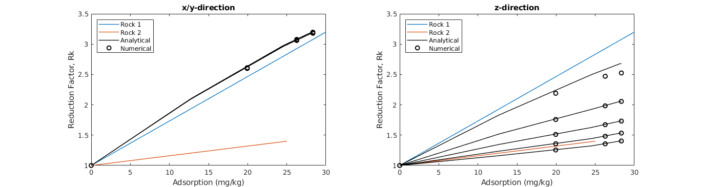
Plot upscaled reduction factor Rk
Finally, we compare the upscaled values of Rk. The plot generated below is equivalent to Figure 3 in [1]. Notice the saturation dependency of the upscaled Rk in the z-direction.
clf;
lw = 1;
colors = lines(numel(updata.krW));
lh = nan(4,1);
dims = [1 3];

% Plot both x- and z-direction. y is equal to x.
for i=1:2
    d = dims(i);
    subplot(1,2,i); hold on;

    % Plot original curves first
    for r=1:2
        lh(r) = plot(fprop.ads{r}(:,2).*(10^6), Rkorg{r}(:,2), ...
                    'Color', colors(r,:), 'LineWidth', lw );
    end

    % Plot analytical upscaling
    c   = updataA.Rk.c;
    ads = interp1(updata.ads(:,1), updata.ads(:,2), c);
    sW  = updata.Rk.s{i}; % Numerical
    for is=1:numel(sW)
        s  = sW(is);
        Rk = nan(1,numel(c));
        for ic=1:numel(c)
            Rk(ic) = interp1(updataA.Rk.s{d}, updataA.Rk.val{d}(:,ic), s);
        end
        lh(3) = plot(ads.*(10^6), Rk, 'k', 'LineWidth', lw );
    end

    % Plot numerical upscaling. Note that the second dimension is z, so we
    % use index i instead of d.
    c   = updata.Rk.c;
    ads = interp1(updata.ads(:,1), updata.ads(:,2), c);
    sW  = updata.Rk.s{i};
    for is=1:numel(sW)
        lh(4) = plot(ads.*(10^6), updata.Rk.val{i}(is,:), 'ko', ...
            'LineWidth', 1.5 );
    end

    if (i==1),title('x/y-direction');else title('z-direction');end
    legend(lh, {'Rock 1','Rock 2','Analytical','Numerical'}, ...
        'Location','NorthWest');
    box on; axis([0 30 1 3.5]);
    xlabel('Adsorption (mg/kg)'); ylabel('Reduction Factor, Rk');
end
One-Phase Block Upscaling Example
Generated from BlockOnePhaseExample.m
Example showing permeability upscaling of a single grid block, i.e., the entire grid G is upscaled to a single coarse cell. The upscaling can be performed using Dirichlet or periodic boundary conditions, or simpler averaging methods may be applied. Step through the blocks of the script.
Add MRST modules
% We rely on the following MRST modules
mrstModule add incomp upscaling steady-state

% In addition, we will use the SPE10 grid as an example model
mrstModule add spe10
Construct a model
We extract a small block from the SPE10 model 1.
% Rock
I = 1:5; J = 30:35; K = 1:5; % Make some selection
rock = getSPE10rock(I, J, K); % Get SPE10 rock

% Grid
cellsize = [20, 10, 2].*ft; % Cell size (ft -> m)
celldim  = [numel(I), numel(J), numel(K)];
physdim  = celldim.*cellsize;
G = cartGrid(celldim, physdim); % Create grid structre
G = computeGeometry(G); % Compute volumes, centroids, etc.
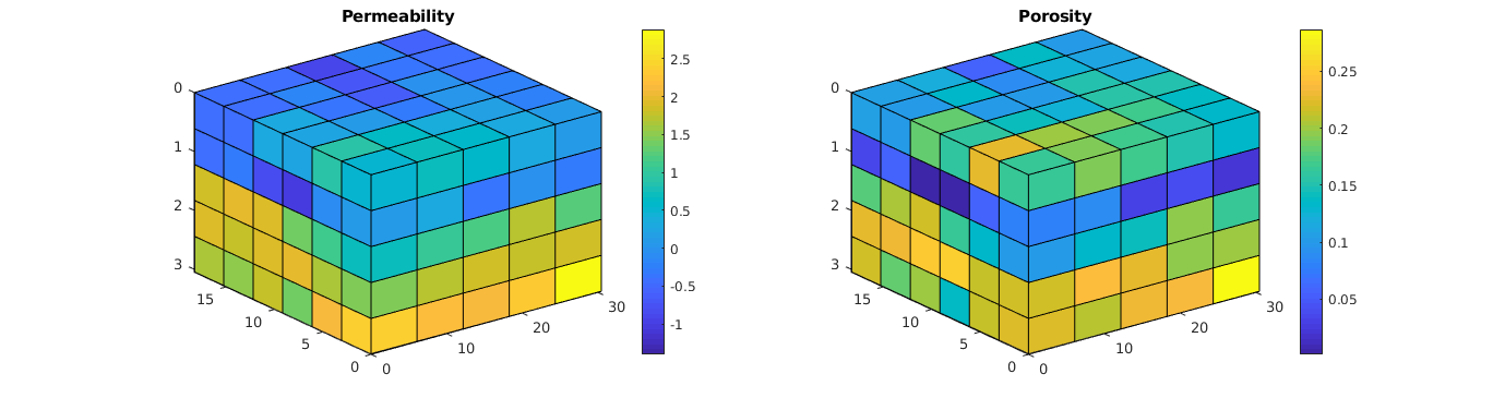
Plot the grid
% Create a new figure and set it wide
close(figure(1)); fh = figure(1);
op = get(fh, 'OuterPosition');
set(fh, 'OuterPosition', op.*[1 1 2.4 1]);

% Permeability on a log-scale
subplot(1,2,1);
plotCellData(G, log10(convertTo(rock.perm(:,1), milli*darcy)) );
view(3); axis tight;
xlabel('x-axis'); ylabel('y-axis'); zlabel('z-axis');
title('Permeability'); colorbar;

% Porosity
subplot(1,2,2);
plotCellData(G, rock.poro); view(3); axis tight;
xlabel('x-axis'); ylabel('y-axis'); zlabel('z-axis');
title('Porosity'); colorbar;

Upscale block using Dirichlet BC
% Create GridBlock: to simplify the passing of arguments in different
% upscaling methods, we create a GridBlock instance which holds the grid,
% the rock, and other properties of the grid block that is to be upscaled.
block = GridBlock(G, rock);

% Upscale permeability: upscaled using Dirichlet boundary conditions, and
% no-flow on the normal boundaries. The upscaled data is returned in a
% structure. This structre can grow as more properties are upscaled.
updata = upAbsPermPres(block);

% Upscale porosity of the block by pore volume averaging
updata = upPoro(block, updata);

% Display the upscaled data
updata %#ok<NOPTS>
updata =

  struct with fields:

    perm: [4.9140e-14 4.4315e-14 1.9735e-19]
    poro: 0.1528
Upscale block using periodic BC
% Create GridBlock with the parameter 'periodic' set to 'true'. The
% GridBlock will then make the grid periodic.
block = GridBlock(G, rock, 'periodic', true);

% Upscale permeability. The function is set up to only return the diagonal
% of the upscaled tensor by default. The previous permeability upscaling is
% replaced.
updata = upAbsPermPres(block, updata) %#ok<NOPTS>

% We can get the full tensor by asking for it.
updata = upAbsPermPres(block, updata, 'fulltensor', true);
updata.perm

% Note that the porosity will not change becuase the grid is periodic.
updata =

  struct with fields:

    perm: [4.6386e-14 4.2023e-14 1.9792e-19]
    poro: 0.1528

...
Using the Upscaler class
Instead of calling the upscaling functions directly, we may use the subclasses of the Upscaling class. For one phase upscaling, we call the class OnePhaseUpscaler.
% Create an instance of the upscaler
upscaler = OnePhaseUpscaler(G, rock);

% Perform the upscaling. The data structure returned contains both the
% permeability and the porosity.
updata = upscaler.upscaleBlock(block) %#ok<NASGU,NOPTS>
updata =

  struct with fields:

    dims: [1 2 3]
    perm: [4.6386e-14 4.2023e-14 1.9792e-19]
    poro: 0.1528
Permeability averaging
We may also choose to use an averaging method to find uspcaled values of the permeability instead of the pressure solver.
% Let us for example compute the arithmetic average.
upscaler.OnePhaseMethod = 'arithmetic';
updata = upscaler.upscaleBlock(block) %#ok<NASGU,NOPTS>

% Another alternative is the combination of harmonic and arithmetic. For
% each different method, observe how the values of the upscaled
% permeability changes.
upscaler.OnePhaseMethod = 'harmonic-arithmetic';
updata = upscaler.upscaleBlock(block) %#ok<NOPTS>
updata =

  struct with fields:

    dims: [1 2 3]
    perm: [6.3091e-14 6.3091e-14 1.3798e-14]
    poro: 0.1528
...
Block Polymer Example
Generated from BlockPolymerExample.m
This example demonstrates polymer upscaling of a single grid block, meaning that the entire grid G is upscaled to a single coarse cell. The upscaling of polymer is described in [1]. First, we upscale the absolute permeability and the relative permeavbilities. Then, the polymer reduction factor Rk is upscaled. The upscaling methodology resebles the upscaling of relative permeability. Step through the code blocks of the script. References: [1] Hilden, Lie and Xavier Raynaud - “Steady State Upscaling of Polymer Flooding”, ECMOR XIV - 14th European conference on the mathematics of oil recovery, 2014.
Add MRST modules
% We rely on the following MRST modules
mrstModule add incomp upscaling ad-props ad-core ad-blackoil steady-state

% In addition, we will use the SPE10 grid as an example model
mrstModule add spe10
Open a new figure and make it wide
fh = figure;
set(fh, 'Name', 'Block Polymer Example', 'NumberTitle', 'off');
op = get(fh, 'OuterPosition');
set(fh, 'OuterPosition', op.*[1 1 2.4 1]);

Construct a model
We extract a small block from the SPE10 model 1.
% Rock
I = 1:5; J = 30:35; K = 1:5; % Make some selection
rock = getSPE10rock(I, J, K); % Get SPE10 rock
rock.poro(rock.poro==0) = min(rock.poro(rock.poro>0)); % Remove zero poro

% Grid
cellsize = [20, 10, 2].*ft; % Cell size (ft -> m)
celldim  = [numel(I), numel(J), numel(K)];
physdim  = celldim.*cellsize;
G = cartGrid(celldim, physdim); % Create grid structre
G = computeGeometry(G); % Compute volumes, centroids, etc.
Plot the grid
% Plot the permeability
clf; subplot(1,2,1);
plotCellData(G, log10(convertTo(rock.perm(:,1), milli*darcy)));
view(3); axis tight; colorbar; title('Permeability');

% Plot the regions
subplot(1,2,2);
plotCellData(G, rock.poro); view(3); axis tight;
colorbar; title('Porosity');
Create two regions
% Create two regions which will have different relative permeability data.
% This will make the relative permeability upscaling more interesting. We
% divide the cells in two equal sizes, based on the value of the
% permeability.
kl = log10(rock.perm(:,1));
regnum = ones(G.cells.num, 1);
regnum(kl<median(kl)) = 2;
Plot the permeability and regions
% Plot the permeability
clf; subplot(1,2,1);
plotCellData(G, log10(convertTo(rock.perm(:,1), milli*darcy)));
view(3); axis tight; colorbar; title('Permeability');

% Plot the regions
subplot(1,2,2);
plotCellData(G, regnum); view(3); axis tight;
colorbar; title('Rock regions');

Create a fluid
We apply some helper functions to help us create an example fluid
% Get a property structure
fprop = getExampleFluidProps(rock, 'satnum', regnum, ...
    'swir', [0.1 0.25], 'sor',[0.14 0.18], 'krWmax', [0.8 0.6], ...
    'nsat', 30, 'polymer', true);

% Create an MRST fluid from the property structure
fluid = initADIFluidOWPolymer(fprop);
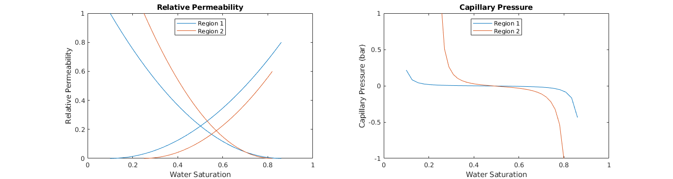
Plot fluid properties
clf;

% Relative permeability
subplot(1,2,1); hold on;
colors = lines(2); lh = nan(2,1);
for r=1:2
    lh(r) = plot(fprop.krW{r}(:,1), fprop.krW{r}(:,2), ...
                'Color', colors(r,:) );
            plot(1-fprop.krO{r}(:,1), fprop.krO{r}(:,2), ...
                'Color', colors(r,:) );
end
box on; axis([0 1 0 1]); title('Relative Permeability');
legend(lh,{'Region 1','Region 2'},'Location','North');
xlabel('Water Saturation'); ylabel('Relative Permeability');

% Capillary pressure
subplot(1,2,2); hold on;
lh = nan(2,1);
for r=1:2
    lh(r) = plot(fprop.pcOW{r}(:,1), fprop.pcOW{r}(:,2)./barsa, ...
                'Color', colors(r,:) );
end
box on; axis([0 1 -1 1]); title('Capillary Pressure');
legend(lh,{'Region 1','Region 2'},'Location','North');
xlabel('Water Saturation'); ylabel('Capillary Pressure (bar)');
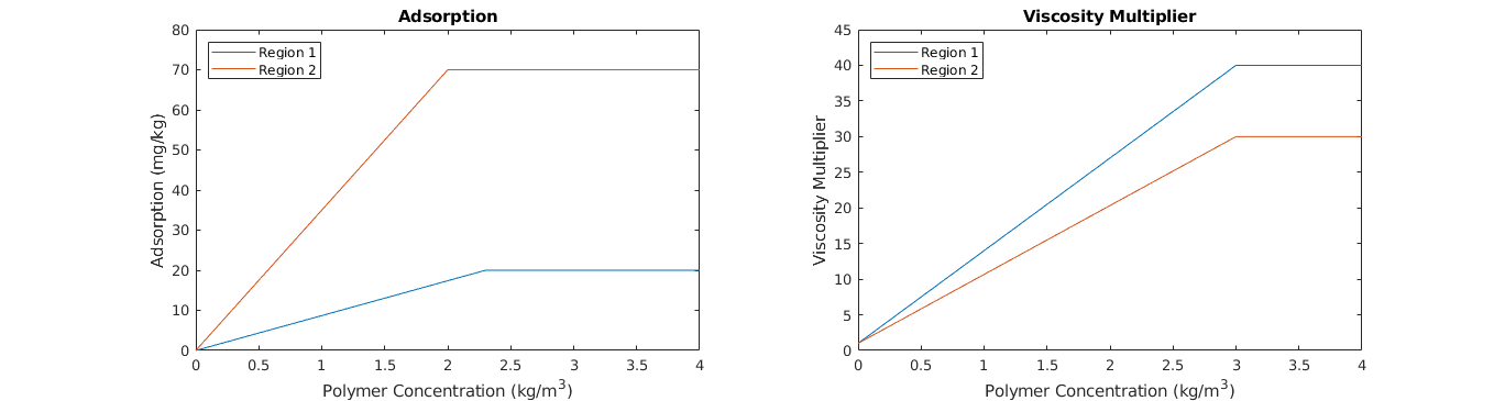
Plot polymer properties
clf;

% Relative permeability
subplot(1,2,1); hold on;
colors = lines(2); lh = nan(2,1);
for r=1:2
    lh(r) = plot(fprop.ads{r}(:,1), fprop.ads{r}(:,2).*(10^6), ...
                'Color', colors(r,:) );
end
box on; title('Adsorption'); axis([0 4 0 80]);
legend(lh,{'Region 1','Region 2'},'Location','NorthWest');
xlabel('Polymer Concentration (kg/m^3)'); ylabel('Adsorption (mg/kg)');

% Capillary pressure
subplot(1,2,2); hold on;
lh = nan(2,1);
for r=1:2
    lh(r) = plot(fprop.muWMult{r}(:,1), fprop.muWMult{r}(:,2), ...
                'Color', colors(r,:) );
end
box on; title('Viscosity Multiplier'); axis([0 4 0 45]);
legend(lh,{'Region 1','Region 2'},'Location','NorthWest');
xlabel('Polymer Concentration (kg/m^3)'); ylabel('Viscosity Multiplier');
Create Block and Upscale Absolute and Relative Permeability
See the exampels BlockOnePhaseExample and BlockTwoPhaseExample for more on one- and two-phase upscaling.
% Create grid block
block = GridBlock(G, rock, 'fluid', fluid);

% Upscale porosity
updata = upPoro(block);

% Upscale absolute permeability
updata = upAbsPermPres(block, updata);

% Upscale relative permeability (using viscous-limit method)
%updata = upRelPerm(block, updata, 'viscous');
Upscale Permeability
updata = upRelPerm(block, updata, 'viscous', 'dims', 1);
Block Two-Phase Example
Generated from BlockTwoPhaseExample.m
This example demonstrates two-phase upscaling of a single grid block, meaning that the entire grid G is upscaled to a single coarse cell. To perform a two-phase upscaling, we must first upscale the absolute permeability (see BlockOnePhaseExample). Subsequently, the relative permeability curves are upscaled. Step through the code blocks of the script.
Add MRST modules
% We rely on the following MRST modules
mrstModule add incomp upscaling ad-props ad-core ad-blackoil steady-state

% In addition, we will use the SPE10 grid as an example model
mrstModule add spe10
Open a wide figure
fn = 44; % Just some arbitrary number
close(figure(fn)); fh = figure(fn);
set(fh, 'Name', 'Block Two-Phase Example', 'NumberTitle', 'off');
op = get(fh, 'OuterPosition');
set(fh, 'OuterPosition', op.*[1 1 2.4 1]);

Construct a model
We extract a small block from the SPE10 model 1.
% Rock
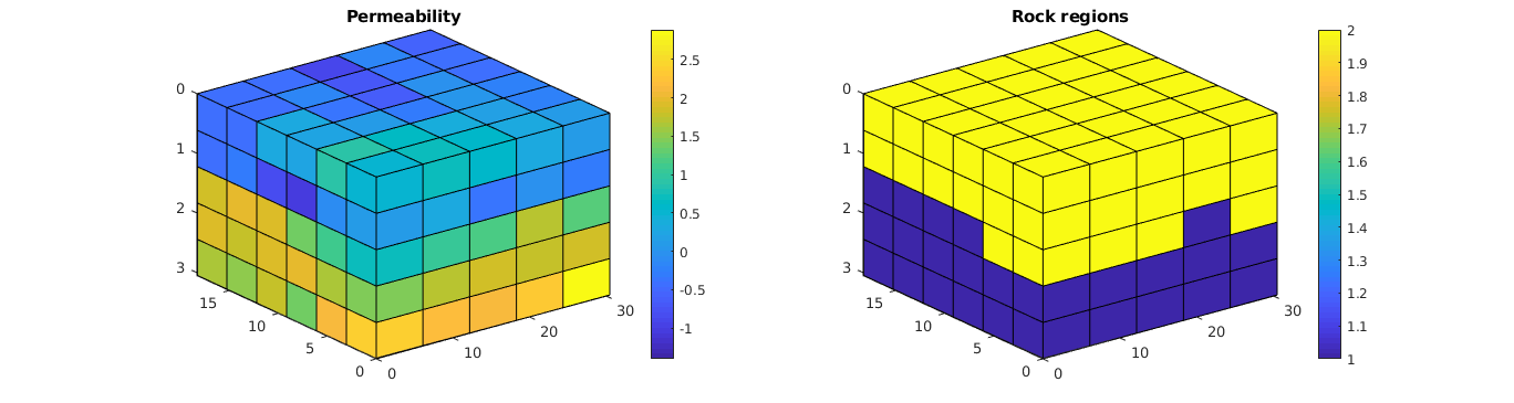
I = 1:5; J = 30:35; K = 1:5; % Make some selection
rock = getSPE10rock(I, J, K); % Get SPE10 rock
rock.poro(rock.poro==0) = min(rock.poro(rock.poro>0)); % Remove zero poro
% Grid
cellsize = [20, 10, 2].*ft; % Cell size (ft -> m)
celldim = [numel(I), numel(J), numel(K)];
physdim = celldim.*cellsize;
G = cartGrid(celldim, physdim); % Create grid structre
G = computeGeometry(G); % Compute volumes, centroids, etc.
Plot the grid
% Plot the permeability
figure(fn); clf; subplot(1,2,1);
plotCellData(G, log10(convertTo(rock.perm(:,1), milli*darcy)));
view(3); axis tight; colorbar; title('Permeability');

% Plot the regions
subplot(1,2,2);
plotCellData(G, rock.poro); view(3); axis tight;
colorbar; title('Porosity');

Create two regions
% Create two regions which will have different relative permeability data.
% This will make the relative permeability upscaling more interesting. We
% divide the cells in two equal sizes, based on the value of the
% permeability.
kl = log10(rock.perm(:,1));
regnum = ones(G.cells.num, 1);
regnum(kl<median(kl)) = 2;
Plot the permeability and regions
% Plot the permeability
clf; subplot(1,2,1);
plotCellData(G, log10(convertTo(rock.perm(:,1), milli*darcy)));
view(3); axis tight; colorbar; title('Permeability');

% Plot the regions
subplot(1,2,2);
plotCellData(G, regnum); view(3); axis tight;
colorbar; title('Rock regions');
Create a fluid
We apply some helper functions to help us create an example fluid
% Get a property structure
fprop = getExampleFluidProps(rock, 'satnum', regnum, ...
    'swir', [0.1 0.25], 'sor',[0.14 0.18], 'krWmax', [0.8 0.6], ...
    'nsat', 30);

% Create an MRST fluid from the property structure
fluid = initADIFluidOW(fprop);
Plot fluid properties
clf;

% Relative permeability
subplot(1,2,1); hold on;
colors = lines(2); lh = nan(2,1);
for r=1:2
    lh(r) = plot(fprop.krW{r}(:,1), fprop.krW{r}(:,2), ...
                'Color', colors(r,:) );
            plot(1-fprop.krO{r}(:,1), fprop.krO{r}(:,2), ...
                'Color', colors(r,:) );
end
box on; axis([0 1 0 1]); title('Relative Permeability');
legend(lh,{'Region 1','Region 2'},'Location','North');
xlabel('Water Saturation'); ylabel('Relative Permeability');

% Capillary pressure
subplot(1,2,2); hold on;
lh = nan(2,1);
for r=1:2
    lh(r) = plot(fprop.pcOW{r}(:,1), fprop.pcOW{r}(:,2)./barsa, ...
                'Color', colors(r,:) );
end
box on; axis([0 1 -1 1]); title('Capillary Pressure');
legend(lh,{'Region 1','Region 2'},'Location','North');
xlabel('Water Saturation'); ylabel('Capillary Pressure (bar)');

Create Block and Upscaled Absolute Permeability
% Create GridBlock: to simplify the passing of arguments in different
% upscaling methods, we create a GridBlock instance which holds the grid,
% the rock, and other properties of the grid block that is to be upscaled.
% For two-phase flow, the block also need to access the fluid structure.
block = GridBlock(G, rock, 'fluid', fluid);

% Upscale porosity
updata = upPoro(block);

% Upscale permeability: we need to upscale the (absolute) permeability
% before upscaling relative permeability. Here, we use Dirichlet boundary
% conditions with no-flow on the normal boundaries.
updata = upAbsPermPres(block, updata) %#ok<NOPTS>
updata =

  struct with fields:

    poro: 0.1529
    perm: [4.9140e-14 4.4315e-14 1.9735e-19]
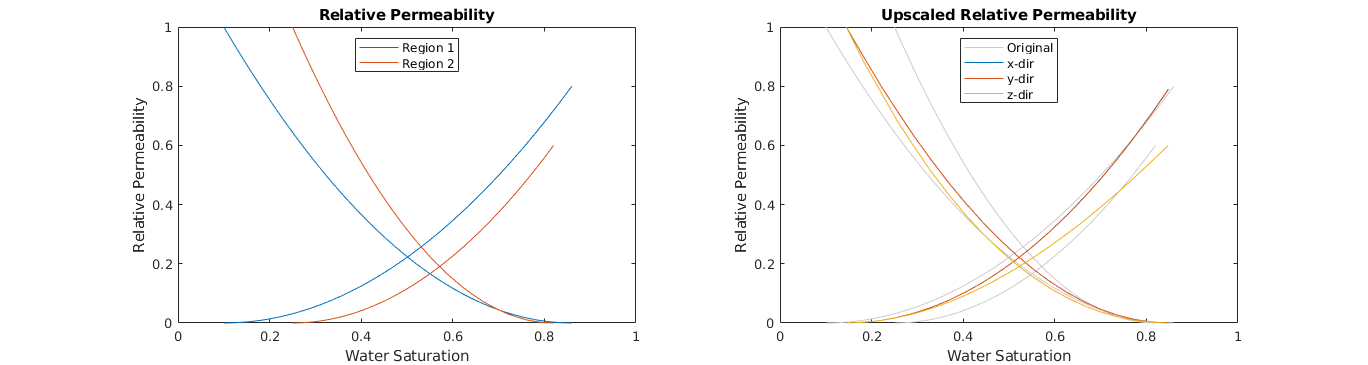
Relative Permeability upscaling - Viscous-Limit method
Let’s start by upscaling relperm using viscous-limit steady-state upscaling. This method assumes the capillary forces are negligable and that the fractional flow is constant in the grid block. If nothing is specified, then the relative permeability is upscaled in each of the three dimensions.
updataVL = upRelPerm(block, updata, 'viscous') %#ok<NOPTS>
updataVL =

  struct with fields:

    poro: 0.1529
    perm: [4.9140e-14 4.4315e-14 1.9735e-19]
     krO: {[20×2 double]  [20×2 double]  [20×2 double]}
...
Plot the upscaled relative permeability
We plot the upscaled curves with the original curves. Observe that the upscaling in x- and y-direction are almost identical, while the z-direction upscaling is clearly different. This is not unusual, as reservoirs often can have some form of horizontal layering. Another point to note, is that for the x- and y-direction, the upscaled curves are closer to the original curves of region 1 than region 2. This can be explained by region 1 having higher absolute permeability, and thus more flow goes through region 1, making this the ‘domonant’ region. Of cource, the above observations will not be valid if the original domain is changed.
subplot(1,2,2); cla; hold on;
lh = nan(numel(updataVL.krW)+1,1);
for r=1:2 % Plot original curves in the backgroudn
    lh(1) = plot(fprop.krW{r}(:,1), fprop.krW{r}(:,2), ...
                'Color', [1 1 1].*0.8 );
            plot(1-fprop.krO{r}(:,1), fprop.krO{r}(:,2), ...
                'Color', [1 1 1].*0.8 );
end
colors = lines(numel(updataVL.krW));
for d=1:numel(updataVL.krW) % Plot the upscaled curves on top
    lh(d+1) = plot(updataVL.krW{d}(:,1), updataVL.krW{d}(:,2), ...
                'Color', colors(d,:) );
            plot(updataVL.krO{d}(:,1), updataVL.krO{d}(:,2), ...
                'Color', colors(d,:) );
end
box on; axis([0 1 0 1]); title('Upscaled Relative Permeability');
legend(lh,{'Original','x-dir','y-dir','z-dir'},'Location','North');
xlabel('Water Saturation'); ylabel('Relative Permeability');
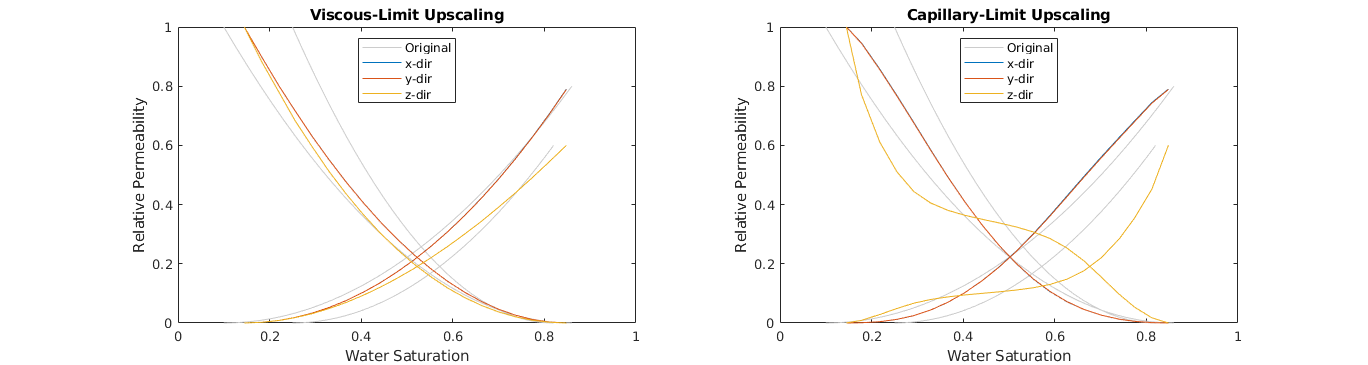
Relative Permeability upscaling - Capillary-Limit method
In the other steady-state limit, capillary-limit upscaling, it is assumed that the velocity is small enough, such that the capillary forces dominate.
% To run the capillary-limit upscaling, we must first upscale the capillary
% pressure curves.
updata = upPcOW(block, updata);

% Then we can upscale the relative permeability
updataCL = upRelPerm(block, updata, 'capillary');
Plot the upscaled relative permeabilitis
clf;

for i = 1:2
    subplot(1,2,i); hold on;
    if i==1
        ud = updataVL; % Left: Viscous-limit upscaled curves
        title('Viscous-Limit Upscaling');
    else
        ud = updataCL; % Right: Capillary-limit upscaled curves
        title('Capillary-Limit Upscaling');
    end
    lh = nan(numel(ud.krW)+1,1);
    for r=1:2 % Plot original curves in the backgroudn
        lh(1) = plot(fprop.krW{r}(:,1), fprop.krW{r}(:,2), ...
                    'Color', [1 1 1].*0.8 );
                plot(1-fprop.krO{r}(:,1), fprop.krO{r}(:,2), ...
                    'Color', [1 1 1].*0.8 );
    end
    colors = lines(numel(ud.krW));
    for d=1:numel(ud.krW) % Plot the upscaled curves on top
        lh(d+1) = plot(ud.krW{d}(:,1), ud.krW{d}(:,2), ...
                    'Color', colors(d,:) );
                plot(ud.krO{d}(:,1), ud.krO{d}(:,2), ...
                    'Color', colors(d,:) );
    end
    box on; axis([0 1 0 1]);
    legend(lh,{'Original','x-dir','y-dir','z-dir'},'Location','North');
    xlabel('Water Saturation'); ylabel('Relative Permeability');
end

% Observe how the two different methods produce different upscaled relative
% permeability curves. Especially in the z-direction, the two methods
% differ significantly in this case.
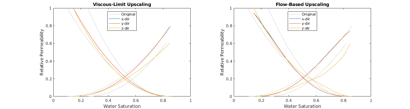
Rate-Dependent Steady-State Upscaling
% The viscous- and capillary-limit methods make simplifications which makes
% it faster to find the satuartion distribution at steady state. However,
% in general for intermediate flow-rates, the saturation distribution at
% steady-state must be computed for each value of the average saturation
% and for each flow direction. This flow-based steady-state upscaling is
% *much* more time-consuming, but may be more accurate if none of the
% limits can be assumed.

% Create a block with periodic grid.
blockP = GridBlock(G, rock, 'fluid', fluid, 'periodic', true);

% Run the upscaling. As the steady-state simulations are time-comsuming, we
% supply the verbose option to get updates printed to the console during
% the upscaling.
updataRD = upRelPerm(blockP, updata, 'flow', 'dp', 1*barsa, ...
    'verbose', true);
Starting relperm upscaling
   #      sW   Time(s)
  1/20   0.14   0.01
  2/20   0.18   2.34
  3/20   0.22   1.81
  4/20   0.26   1.93
  5/20   0.29   1.75
...
Plot the upscaled relative permeabilitis
We compare the uscaled curves from the periodic flow-based steady-state upscaling with the viscous-limit upscaling.
clf;
for i = 1:2
    subplot(1,2,i); hold on;
    if i==1
        ud = updataVL; % Left: Viscous-limit upscaled curves
        title('Viscous-Limit Upscaling');
    else
        ud = updataRD; % Right: Flow-based upscaling curves
        title('Flow-Based Upscaling');
    end
    lh = nan(numel(ud.krW)+1,1);
    for r=1:2 % Plot original curves in the backgroudn
        lh(1) = plot(fprop.krW{r}(:,1), fprop.krW{r}(:,2), ...
                    'Color', [1 1 1].*0.8 );
                plot(1-fprop.krO{r}(:,1), fprop.krO{r}(:,2), ...
                    'Color', [1 1 1].*0.8 );
    end
    colors = lines(numel(ud.krW));
    for d=1:numel(ud.krW) % Plot the upscaled curves on top
        lh(d+1) = plot(ud.krW{d}(:,1), ud.krW{d}(:,2), ...
                    'Color', colors(d,:) );
                plot(ud.krO{d}(:,1), ud.krO{d}(:,2), ...
                    'Color', colors(d,:) );
    end
    box on; axis([0 1 0 1]);
    legend(lh,{'Original','x-dir','y-dir','z-dir'},'Location','North');
    xlabel('Water Saturation'); ylabel('Relative Permeability');
end