`geochemistry`: Surface geochemistry¶

# README #

The matlab-geoChemistry repository contains tools for the solution of equilibrium geochemical systems including aqueous and surface chemistry for use in batch and transport settings.

### Summary ###

The main function of this repository, ChemicalModel, allows the creation and solution of arbitrarily complex chemistry systems including equilibrium aqueous speciation, surface complexation, ion exchange, redox chemistry, dissolution/precipitation and equilbrium with gas phases. The function leverages the tools developed by the SINTEF [MRST team](http://www.sintef.no/projectweb/mrst/) including [automatic differentiation](https://en.wikipedia.org/wiki/Automatic_differentiation). The chemical model created can be used to calculate batch reaction or can be coupled to flow within MRST. See the user guide pdf for details on use, equations, examples, and benchmarks.

Models supported:

aqueous speciation
aqueous activity
surface chemistry
- triple layer model
- diffuse layer model
- basic stern model
- constant capacitance model
- ion exchange
dissolution/precipitation
gas phase equilibrium

### Installation ###

Install [MRST](http://www.sintef.no/projectweb/mrst/download/).
Add the matlab-geoChemistry folder to the “modules” folder of MRST.
Create a file named startup_user.m within the MRST folder, at the same level as startup.m.

4. In startup_user.m add the line¶

mrstPath(‘register’, ‘geochemistry’, ‘path/to/repo/matlab-geochemistry’)¶

### Use ###

Once MRST is installed and made aware of the location of matlab-geoChemistry the module can be used like any other MRST module.

Before any script that relies on the repository is run, MRST must be started. This is done by running the file startup.m which is loacted inside of your MRST directory.

To use the geochemistry module in a Matlab script include the command

mrstModule add geochemistry ad-core¶

this will make the contents of the geochemistry directory available in the workspace.

### in progress ### * address slight mismatch between phreeqc and match for saturation index * release transport examples

changeUnits(states, fields, unit_conv)¶

changeUnits converts the specified fields in states to the specified units.

Synopsis:

[state] = changeUnits(state, fields, unit)

Parameters:

state –

The state structure produced by ChemicalModel/initstate. State: must be populated by the named variable before they can be retrived.
fields - Name of the fields for which the unit change is to occur. Can: be a string or cell array of strings.
unit - Numeric value of unit conversion. If numel(unit) == 1 and fields: has multple entries then the one value of unit will be applied to all fields. Otherwise if fields is a cell with multple entries then fields and unit must have the same size, numel(unit) == numel(fields).unit_conv = unit_conv.^-1;

Returns: state – the state variable with the fields state.fields converted from SI units to the units specified in units

Example:

% change the units of a single fields

      [state] = changeUnits(state, 'activities', mol/litre)

%change the units of a multiple fields

      fields = {'acitivities', 'surfaceCharges'}
      units = [mol/litre, mili*Coulumb/(nano*meter)^2];

      state = chem.getProps(state, fields, units);

If state is a cell array of structures the function will loop over each cell.

The numeric value of the unit conversion must be defined. There is a bank
of unit conversions within the release.

Examples¶

clear;
close all;

load adi and geochemistry module¶

Generated from alkalinity.m

mrstModule add ad-core geochemistry
mrstVerbose on

define the chemical model¶

here we choose CO3, H2O and alkalaninity as inputs

% define elements names
elements = {'H', 'CO3*','O'};

% define chemical species
species = {'H+','H2CO3','HCO3-','CO3-2','H2O*','OH-'};

% list chemical reactions
reactions ={'H2CO3  = H+ + HCO3- ',         10^2*mol/litre,...
            'HCO3- = H+ + CO3-2',           10^-1*mol/litre,...
            'H2O = H+ + OH-',               10^-14*mol/litre};

% define any linear combinations
combinations = {'Alk*', 'HCO3- + 2*CO3-2 + OH- - H+' };

% instantiate the chemical model
chemsys = ChemicalSystem(elements, species, reactions, 'comb', combinations);

% print the chemical system
chemsys.printChemicalSystem;

% Setup model
chemmodel = ChemicalModel(chemsys);

===========================================================
|Equations      |    H+| H2CO3| HCO3-| CO3-2|   H2O|   OH-|
===========================================================
|sum(H)         |     1|     2|     1|     0|     2|     1|
|sum(CO3)       |     0|     1|     1|     1|     0|     0|
|sum(O)         |     0|     0|     0|     0|     1|     1|
===========================================================
...

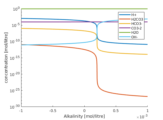
solve the chemical system given inputs¶

here we vary alkalinity and keep carbon and water content constant

n = 1000;

C = 1e-4.*ones(n,1);
H2O = ones(n,1);
Alk = linspace(-10^-3, 10^-3,n)';

userInput = [C H2O Alk]*mol/litre;

tic
[state, report, model] = chemmodel.initState(userInput);
toc;

state = changeUnits(state, {'species'}, mol/litre);

% plot the results
figure; hold on;
plot(Alk, state.species, 'linewidth', 2);
set(gca,'yscale', 'log')
xlabel('Alkalinity [mol/litre]');
ylabel('concentration [mol/litre]');

legend(chemsys.speciesNames)

Computing initial guess...
============================================================================================================================================================================
| It # | H2CO3=H++HCO3- (cell) | HCO3-=H++CO3-2 (cell) | H2O=H++OH- (cell) | Conservation of H (cell) | Conservation of CO3 (cell) | Conservation of O (cell) | Alk (cell) |
============================================================================================================================================================================
|    1 | 4.61e+00              | 2.30e+00              | 3.22e+01          | 1.95e+00                 | 1.03e+01                   | 6.93e-01                 | 3.00e+03   |
|    2 | 3.53e+00              | 9.83e+00              |*3.55e-15          | 1.22e+01                 | 9.30e-02                   | 8.19e+00                 | 1.21e+00   |
|    3 | 3.91e+00              | 8.26e+00              | 1.20e+02          | 6.93e-01                 | 9.25e-01                   | 6.93e-01                 | 2.00e+03   |
|    4 | 2.58e+02              | 1.76e+00              | 4.49e+02          | 4.06e-01                 | 6.06e-01                   | 6.93e-01                 | 1.00e+03   |
...

Copyright notice¶

clear;
close all;

load adi and geochemistry module¶

Generated from constantCapacitance.m

mrstModule add ad-core geochemistry
mrstVerbose on

generate chemical system¶

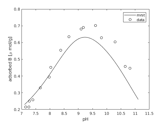
here we look at boron sorption onto the silica surface. we are keeping Na, Cl, B, H+ and H2O concentrations as inputs

% define elements
elements = {'O', 'H', 'Na*', 'Cl*', 'B*'};

species = {'H+*', 'OH-', 'Na+', 'Cl-', 'NaCl', 'H2O*',...
             'H3BO3', 'H4BO4-',...
             '>SO-' '>SOH', '>SOH2+','>SOH3BO3-'};

reactions ={'H2O  = H+  + OH- ',              10^-14*mol/litre, ...
            'NaCl = Na+ + Cl-',               10^1*mol/litre,...
            'H3BO3 + H2O = H4BO4- + H+',      10^-9.2,...
            '>SOH + H+ = >SOH2+',             10^8.31/(mol/litre),...
            '>SOH = >SO- + H+',               10^-11.82*mol/litre,...
            '>SOH + H3BO3 = >SOH3BO3- + H+'    10^-8.2};

% define surface information. Here we describe the surface with the
% constant capacitance model with a capacitance of 1.06 after the values in
% Goldberg et al 2000
geometry = [2.31*site/(nano*meter)^2 59*meter^2/gram 200*gram/litre];
sInfo = {geometry, 'ccm', 1.06};
surfaces ={ '>SO', sInfo};

% instantiate chemical model
chemsys = ChemicalSystem(elements, species, reactions, 'surf', surfaces);

% print the chemical system
chemsys.printChemicalSystem;

% Setup model
chemmodel = ChemicalModel(chemsys);

=========================================================================================================================================================================
|Equations               |        H+|       OH-|       Na+|       Cl-|      NaCl|       H2O|     H3BO3|    H4BO4-|      >SO-|      >SOH|    >SOH2+| >SOH3BO3-|  >SO_ePsi|
=========================================================================================================================================================================
|sum(O)                  |         0|         1|         0|         0|         0|         1|         3|         4|         0|         0|         0|         3|         0|
|sum(H)                  |         1|         1|         0|         0|         0|         2|         3|         4|         0|         1|         2|         3|         0|
|sum(Na)                 |         0|         0|         1|         0|         1|         0|         0|         0|         0|         0|         0|         0|         0|
|sum(Cl)                 |         0|         0|         0|         1|         1|         0|         0|         0|         0|         0|         0|         0|         0|
...

define input parameters¶

here we vary the pH of the system

n = 200;

Na  = 1e-1.*ones(n,1);
Cl  = 1e-1.*ones(n,1);
B   = 4.63e-4.*ones(n,1);
H2O = ones(n,1);
H   = logspace(-7,-11, n)';

userInput = [Na Cl B H H2O]*mol/litre;

solve the chemical system¶

[state, report, model] = chemmodel.initState(userInput, 'charge', 'Cl');

Computing initial guess...
====================================================================================================================================================================================================================================================================================================================================
| It # | H2O=H++OH- (cell) | NaCl=Na++Cl- (cell) | H3BO3+H2O=H4BO4-+H+ (cell) | >SOH+H+=>SOH2+ (cell) | >SOH=>SO-+H+ (cell) | >SOH+H3BO3=>SOH3BO3-+H+ (cell) | Conservation of O (cell) | Conservation of H (cell) | Conservation of Na (cell) | Conservation of Cl (cell) | Conservation of B (cell) | Conservation of >SO (cell) |
====================================================================================================================================================================================================================================================================================================================================
|    1 | 1.61e+01          | 2.30e+00            | 5.07e+00                   | 6.19e+00              | 1.11e+01            | 6.45e+00                       | 2.48e+00                 | 2.77e+00                 | 3.00e+00                  | 3.00e+00                  | 8.78e+00                 | 4.48e+00                   |
|    2 |*1.78e-15          | 2.15e+00            | 1.59e+00                   | 3.71e+00              | 3.29e+00            | 4.88e+00                       | 6.37e+00                 | 4.77e+00                 | 8.20e-02                  | 8.20e-02                  | 6.41e-01                 | 3.43e-01                   |
|    3 |*0.00e+00          | 1.61e-01            | 9.52e-01                   | 1.39e+00              | 8.91e-01            | 9.52e-01                       | 1.56e-03                 | 1.62e-02                 | 1.17e-02                  | 1.17e-02                  | 6.89e-01                 | 3.33e-01                   |
|    4 |*0.00e+00          |*2.50e-16            | 9.10e-04                   | 4.82e-02              |*1.78e-15            | 9.10e-04                       | 5.86e-04                 | 2.46e-03                 | 1.59e-04                  | 1.59e-04                  | 1.07e-01                 | 7.17e-02                   |
...

calculate auxillary information¶

surface charge, potential, aqueous and surface concentrations can be calculated with tools built into ChemicalModel

[state, chemmodel] = chemmodel.updateActivities(state);
[state, chemmodel] = chemmodel.updateChargeBalance(state);
[state, chemmodel] = chemmodel.updateSurfacePotentials(state);
[state, chemmodel] = chemmodel.updateAqueousConcentrations(state);
[state, chemmodel] = chemmodel.updateSurfaceConcentrations(state);


state = changeUnits(state, {'species','activities','elements','surfaceConcentrations'}, mol/litre);
pH = -log10(getProp(chemmodel, state, 'aH+'));

data from Goldberg¶

data is from Goldberg et al. Soil Sci. Soc. Am. J. 64:1356-1363 (2000)

GB =   [7.145895      0.2151590
        7.259432      0.2151301
        7.277191      0.2502701
        7.399525      0.2578790
        7.662131      0.3296291
        7.977074      0.3937258
        8.029960      0.4517771
        8.380156      0.5540653
        8.669038      0.6349768
        9.097366      0.6807084
        9.176045      0.6898564
        9.604094      0.7019716
        9.813089      0.6285734
        10.29323      0.6040028
        10.65009      0.4572219
        10.81594      0.4464835];

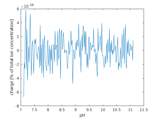
plot the results¶

figure; hold on; box on;
plot(pH, state.chargeBalance)
xlabel('pH')
ylabel('charge [% of total ion concentration]');

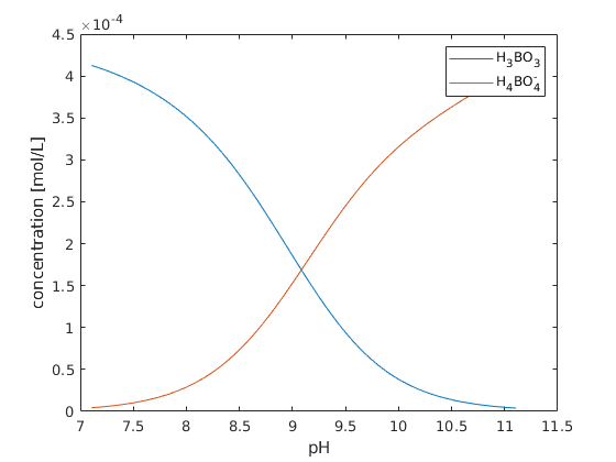
% aqueous components
figure; hold on; box on;
plot(pH, chemmodel.getProp(state, 'H3BO3'));
plot(pH,  chemmodel.getProp(state, 'H4BO4-'));
legend('H_3BO_3','H_4BO_4^-');

xlabel('pH');
ylabel('concentration [mol/L]');

% surface components
figure; hold on; box on;
plot(pH, chemmodel.getProp(state, '>SOH3BO3-')/200*1e6, '-k')
plot(GB(:,1), GB(:,2), 'ok');
legend('mrst', 'data')

xlabel('pH')
ylabel('adsorbed B [\mu mol/g]');

Copyright notice¶

clear;
close all;

add adi and geochemistry modules¶

Generated from ionExchange.m

mrstModule add geochemistry ad-core
mrstVerbose on

instantiate the chemical model¶

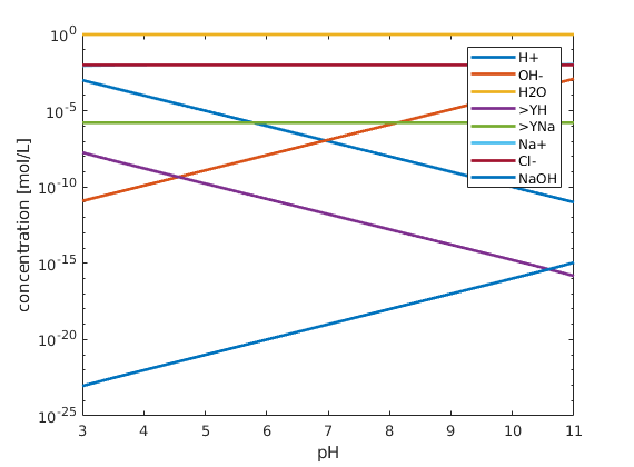
here we look at the competetive sorption of sodium and protons for an ionexhcnage surface. ChemicalModel will verify that surfaces that are designated as ion exchange surfaces do not contain species with a charge

elements = {'O', 'H', 'Na*', 'Cl*'};

species = {'H+*', 'OH-', 'H2O*', '>YH', '>YNa', 'Na+', 'Cl-','NaOH'};

reactions = {'H2O  = H+  + OH- ',           10^-14*mol/litre, ...
             '>YH + Na+ = >YNa + H+',       10^1,...
             'NaOH = Na+ + OH-',            10^10*mol/litre};

surfInfo = {'>Y', {[1*site/(nano*meter)^2 1*meter^2/gram 1*gram/litre], 'ie'}};

chemsys = ChemicalSystem(elements, species, reactions, 'surfaces', surfInfo);

% print the chemical system
chemsys.printChemicalSystem;

% Setup model
chemmodel = ChemicalModel(chemsys);

==================================================================
|Equations       |   H+|  OH-|  H2O|  >YH| >YNa|  Na+|  Cl-| NaOH|
==================================================================
|sum(O)          |    0|    1|    1|    0|    0|    0|    0|    1|
|sum(H)          |    1|    1|    2|    1|    0|    0|    0|    1|
|sum(Na)         |    0|    0|    0|    0|    1|    1|    0|    1|
|sum(Cl)         |    0|    0|    0|    0|    0|    0|    1|    0|
...

specify inputs¶

here we vary pH

n = 100;

H2O = ones(n,1);
H   = logspace(-3, -11,n)';
Na  = 1e-2*ones(n,1);
Cl  = Na;

inputs = [Na, Cl, H, H2O]*mol/litre;

solve the chemical system¶

here we specify that charge balance should be enforced by giving the name/value pair. The total amount of sodium will be varied in order for the charge balance equation to be satisfied

[state, report, chemmodel] = chemmodel.initState(inputs, 'chargeBalance', 'Na');

Computing initial guess...
=====================================================================================================================================================================================================================
| It # | H2O=H++OH- (cell) | >YH+Na+=>YNa+H+ (cell) | NaOH=Na++OH- (cell) | Conservation of O (cell) | Conservation of H (cell) | Conservation of Na (cell) | Conservation of Cl (cell) | Conservation of >Y (cell) |
=====================================================================================================================================================================================================================
|    1 | 2.53e+01          | 2.76e+01               | 2.30e+01            | 1.10e+00                 | 1.61e+00                 | 5.70e+00                  | 4.61e+00                  | 1.40e+01                  |
|    2 | 3.89e+00          | 8.82e+00               | 2.09e+01            | 1.80e+01                 | 1.59e+01                 | 1.66e-04                  |*4.44e-16                  | 1.48e-06                  |
|    3 |*0.00e+00          |*1.86e-07               |*7.11e-15            | 9.00e-04                 | 4.50e-04                 |*1.60e-08                  |*0.00e+00                  | 9.94e-03                  |
|    4 |*0.00e+00          |*3.55e-15               |*7.11e-15            |*0.00e+00                 |*4.09e-13                 |*8.17e-09                  |*0.00e+00                  |*1.33e-14                  |
...

process the data¶

state = changeUnits(state, {'elements','species'}, mol/litre );

[state, chemmodel] = chemmodel.updateActivities(state);

pH = -log10(getProp(chemmodel, state, 'aH+'));

plot the results¶

figure; hold on; box on;
plot(pH, state.species, 'linewidth', 2)

xlabel('pH')
ylabel('concentration [mol/L]');
set(gca, 'yscale', 'log');
legend(chemsys.speciesNames)
xlim([3 11])

Copyright notice¶

clear;
close all;

load adi and geochemistry module¶

Generated from phases.m

mrstModule add ad-core geochemistry
mrstVerbose on

instantiate the chemical system¶

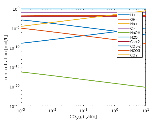
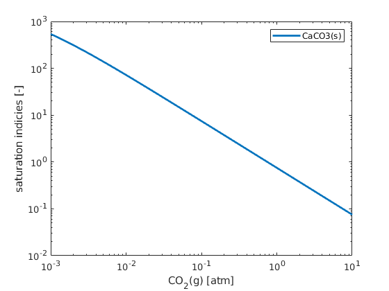
here we look at carbonate speciation with calcite and CO2(g) as non aquoeus phases. We choose the partial pressure of CO2 as an input by appending an asterisk to the name

elements = {'O', 'H', 'Na*', 'Cl*', 'Ca*', 'C'};

species = {'H+*', 'OH-', 'Na+', 'Cl-', 'NaOH', 'H2O*',...
             'Ca+2', 'CO3-2', 'HCO3-', 'CO2',...
             'CaCO3(s)', 'CO2(g)*'};

reactions ={'H2O  = H+  + OH- ',            10^-14*mol/litre, ...
            'NaOH = Na+ + OH-',             10^10*mol/litre,...
            'CaCO3(s) = CO3-2 + Ca+2',      10^-8.48*(mol/litre)^2,...
            'CO3-2 + H+ = HCO3-',           10^10.329/(mol/litre),...
            'CO3-2 + 2*H+ = CO2 + H2O',     10^16.681/(mol/litre),...
            'CO2 = CO2(g)',                 10^1.468*atm/(mol/litre)};

chemsys = ChemicalSystem(elements, species, reactions);

% print the chemical system
chemsys.printChemicalSystem;

% Setup model
chemmodel = ChemicalModel(chemsys);

==============================================================================================================================================
|Equations           |       H+|      OH-|      Na+|      Cl-|     NaOH|      H2O|     Ca+2|    CO3-2|    HCO3-|      CO2| CaCO3(s)|   CO2(g)|
==============================================================================================================================================
|sum(O)              |        0|        1|        0|        0|        1|        1|        0|        3|        3|        2|        3|        2|
|sum(H)              |        1|        1|        0|        0|        1|        2|        0|        0|        1|        0|        0|        0|
|sum(Na)             |        0|        0|        1|        0|        1|        0|        0|        0|        0|        0|        0|        0|
|sum(Cl)             |        0|        0|        0|        1|        0|        0|        0|        0|        0|        0|        0|        0|
...

specify inputs¶

here we vary the partial pressure of CO2 from 1e-3 atm to 3 atm

n = 100;

Na = 1e-1*ones(n,1)*mol/litre;
Cl = 1e-1*ones(n,1)*mol/litre;
H = 1e-4*ones(n,1)*mol/litre;
H2O = ones(n,1)*mol/litre;
Ca = 1e-2*ones(n,1)*mol/litre;
CO2 = logspace(-3, 1, n)'*atm;

solve chemical system given inputs¶

state = chemmodel.initState([Na, Cl, Ca, H, H2O, CO2], 'charge','H+');

Warning: Using any quantity other than a total element concentration as a charge
balance can yield unexpected results.
Computing initial guess...
============================================================================================================================================================================================================================================================================================================================
| It # | H2O=H++OH- (cell) | NaOH=Na++OH- (cell) | CaCO3(s)=CO3-2+Ca+2 (cell) | CO3-2+H+=HCO3- (cell) | CO3-2+2*H+=CO2+H2O (cell) | CO2=CO2(g) (cell) | Conservation of O (cell) | Conservation of H (cell) | Conservation of Na (cell) | Conservation of Cl (cell) | Conservation of Ca (cell) | Conservation of C (cell) |
============================================================================================================================================================================================================================================================================================================================
|    1 | 2.30e+01          | 2.30e+01            | 2.18e+01                   | 1.46e+01              | 2.00e+01                  | 1.03e+01          | 2.40e+00                 | 1.61e+00                 | 3.00e+00                  | 2.30e+00                  | 4.61e+00                  | 1.10e+00                 |
|    2 |*0.00e+00          | 2.23e+01            |*5.33e-15                   | 4.38e+00              | 9.39e+00                  | 9.39e+00          | 1.65e+01                 | 1.20e+01                 |*5.00e-11                  |*0.00e+00                  |*4.44e-16                  | 1.51e+00                 |
...

process data¶

state = changeUnits(state, {'elements','species','partialPressures'}, [mol/litre, mol/litre, atm] );

[state, chemmodel] = chemmodel.updateActivities(state);

plot the results¶

figure; hold on; box on;
plot(CO2/atm, state.species, 'linewidth', 2)
set(gca, 'xscale','log');

xlabel('CO_2(g) [atm]')
ylabel('concentration [mol/L]');
set(gca, 'yscale', 'log');
legend(chemsys.speciesNames)

figure; hold on; box on;
plot(CO2/atm, state.saturationIndicies, 'linewidth', 2)
set(gca, 'xscale','log');

xlabel('CO_2(g) [atm]')
ylabel('saturation indicies [-]');
set(gca, 'yscale', 'log');
legend(chemsys.solidNames)

Copyright notice¶

clear;
close all;

Add geochemistry and automatic differentiation modules¶

Generated from redoxChemistry.m

mrstModule add ad-core geochemistry
mrstVerbose on

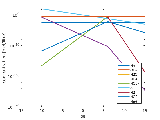
instantiate chemical model¶

here we look at the pe dependent speciation of nitrogen. We are choosing total nitrogen, electron, sodium, H+ and H2O concentrations as inputs.

elements = {'O', 'H', 'N*', 'e*','Na*'};

species = {'H+*', 'OH-', 'H2O*',...
            'NH4+', 'NO3-', 'e-','N2', 'NO2-','Na+'};

reactions ={'H2O  = H+  + OH-',                       10^-14*mol/litre,...
            'NO3- + 10*H+ + 8*e- = NH4+ + 3*H2O',     10^119./(mol/litre)^15,...
            'NO3- + 2*H+ + 2*e- = NO2- + H2O',        10^28./(mol/litre)^3,...
            '2*NO3- + 12*H+ + 10*e- = N2 + 6*H2O',    10^(2*103)./(mol/litre)^17};

chemsys = ChemicalSystem(elements, species, reactions);

% print the chemical system
chemsys.printChemicalSystem;

% Setup model
chemmodel = ChemicalModel(chemsys);

====================================================================================
|Equations                   |   H+|  OH-|  H2O| NH4+| NO3-|   e-|   N2| NO2-|  Na+|
====================================================================================
|sum(O)                      |    0|    1|    1|    0|    3|    0|    0|    2|    0|
|sum(H)                      |    1|    1|    2|    4|    0|    0|    0|    0|    0|
|sum(N)                      |    0|    0|    0|    1|    1|    0|    2|    1|    0|
|sum(e)                      |    0|    0|    0|    0|    0|    1|    0|    0|    0|
...

define input values¶

here we look at the speciation as a function of a range in electron concentration

n = 100;

N = 1e-3*ones(n,1);
e = logspace(-15, 10, n)';
H = 1e-7*ones(n,1);
H2O = ones(n,1);
Na = 1e-2*ones(n,1);

solve the chemical system¶

[state, report] = chemmodel.initState([N e Na H H2O]*mol/litre,'charge','H+');

Warning: Using any quantity other than a total element concentration as a charge
balance can yield unexpected results.
Computing initial guess...
==============================================================================================================================================================================================================================================================================
| It # | H2O=H++OH- (cell) | NO3-+10*H++8*e-=NH4++3*H2O (cell) | NO3-+2*H++2*e-=NO2-+H2O (cell) | 2*NO3-+12*H++10*e-=N2+6*H2O (cell) | Conservation of O (cell) | Conservation of H (cell) | Conservation of N (cell) | Conservation of e (cell) | Conservation of Na (cell) |
==============================================================================================================================================================================================================================================================================
|    1 | 1.61e+01          | 1.13e+02                          | 3.22e+01                       | 2.81e+02                           | 1.95e+00                 | 1.95e+00                 | 8.52e+00                 | 3.45e+01                 | 4.61e+00                  |
|    2 | 1.09e+02          | 9.82e+01                          | 3.68e+01                       | 1.07e+02                           | 1.25e+02                 | 7.11e+01                 | 1.10e+00                 |*3.55e-15                 |*4.44e-16                  |
...

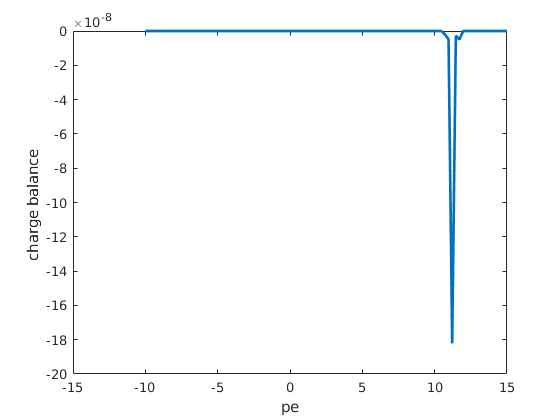
calculate acitivities and charge balance¶

[state, chemmodel] = chemmodel.updateActivities(state);
[state, chemmodel] = chemmodel.updateChargeBalance(state);

state = changeUnits(state, {'species', 'activities'}, mol/litre);

pe = -log10(chemmodel.getProp(state, 'ae-'));

visualize the results¶

figure;
plot(pe, state.species, 'linewidth', 2);
set(gca, 'yscale', 'log');
ylabel('concentration [mol/litre]');
xlabel('pe');
legend(chemsys.speciesNames, 'location', 'southeast');

figure;
plot(pe, state.chargeBalance, 'linewidth', 2);
ylabel('charge balance ');
xlabel('pe');

Copyright notice¶

clear;
close all;

load ad and geochemistry modules¶

Generated from simpleSystem.m

mrstModule add geochemistry ad-core
mrstVerbose on

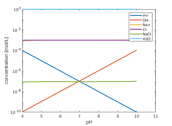
generate chemical system object¶

here we look at a simple example of aqueous speciation of sodium, protons, and chlorine

elements = {'O', 'H', 'Na*', 'Cl*'};

species = {'H+*', 'OH-', 'Na+', 'Cl-', 'NaCl', 'H2O*'};

reactions = {'H2O  = H+  + OH- ', 10^-14*mol/litre, ...
             'NaCl = Na+ + Cl-',  10^1*mol/litre};

chemsys = ChemicalSystem(elements, species, reactions);

chemsys.printChemicalSystem;

===================================================
|Equations    |   H+|  OH-|  Na+|  Cl-| NaCl|  H2O|
===================================================
|sum(O)       |    0|    1|    0|    0|    0|    1|
|sum(H)       |    1|    1|    0|    0|    0|    2|
|sum(Na)      |    0|    0|    1|    0|    1|    0|
|sum(Cl)      |    0|    0|    0|    1|    1|    0|
...

define the input¶

n = 100;

Na  = ones(n,1)*milli*mol/litre;
Cl  = ones(n,1)*milli*mol/litre;
H2O = ones(n,1)*mol/litre;
H   = logspace(-4, -10, n)'*mol/litre;

inputs = [Na, Cl, H, H2O];

solve the chemical system¶

chemmodel = ChemicalModel(chemsys);
[state, report, chem] = chemmodel.initState(inputs, 'chargeBalance', 'Na');

Computing initial guess...
================================================================================================================================================================
| It # | H2O=H++OH- (cell) | NaCl=Na++Cl- (cell) | Conservation of O (cell) | Conservation of H (cell) | Conservation of Na (cell) | Conservation of Cl (cell) |
================================================================================================================================================================
|    1 | 2.30e+01          | 2.30e+00            | 6.93e-01                 | 1.10e+00                 | 7.60e+00                  | 7.60e+00                  |
|    2 |*1.78e-15          | 5.22e+00            | 1.08e+01                 | 7.27e+00                 | 1.83e-02                  | 1.83e-02                  |
|    3 |*0.00e+00          | 1.49e-01            |*2.66e-15                 |*8.88e-16                 | 1.16e-04                  | 1.16e-04                  |
|    4 |*0.00e+00          |*0.00e+00            |*0.00e+00                 |*0.00e+00                 | 1.24e-06                  | 1.24e-06                  |
...

process the data¶

state = changeUnits(state, {'elements','species'}, mol/litre );

[state, chem] = chemmodel.updateActivities(state);

pH = -log10(getProp(chem, state, 'aH+'));

plot the results¶

figure; hold on; box on;
plot(pH, state.species, 'linewidth',2)

xlabel('pH')
ylabel('concentration [mol/L]');
set(gca, 'yscale', 'log');
legend(chemsys.speciesNames)

Copyright notice¶

clear;
close all;

load adi and geochemistry module¶

Generated from tripleLayerExample.m

mrstModule add ad-core geochemistry
mrstVerbose on

generate chemical system¶

here we look at an amphoteric surface with the sorption of Na and Cl

% define elements names
elements = {'O', 'H', 'Na*', 'Cl*'};

% define chemical species
species = {'H+*', 'OH-', 'Na+', 'Cl-', 'NaCl', 'H2O*',...
             '>SO-', '>SOH', '>SOH2+', '>SONa', '>SOH2Cl'};

% list chemical reactions
reactions ={'H2O  = H+  + OH- ',          10^-14*mol/litre, ...
            'NaCl = Na+ + Cl-',           10^1*mol/litre,...
            '>SOH = >SO- + H+',           10^-7.5*mol/litre,...
            '>SOH + H+ = >SOH2+',         10^2/(mol/litre),...
            '>SO- + Na+ = >SONa',         10^-1.9/(mol/litre),...
            '>SOH2+ + Cl- = >SOH2Cl',     10^-1.9/(mol/litre)};

% define the surface, here we choose a triple layer model to describe the
% surface. Outersphere complexes like >SONa and >SOH2Cl are defined by
% defining their charge contributions to the inner and outer helmholtz plane

geometry = [2*site/(nano*meter)^2 50e-3*meter^2/gram 5e3*gram/litre];
sioInfo = {geometry, 'tlm', [1 0.2]/meter^2,      '>SONa',   [-1 1], '>SOH2Cl',[1 -1]};
surfaces ={ '>SO', sioInfo };

% instantiate the chemical model
chemsys = ChemicalSystem(elements, species, reactions, 'surf', surfaces);


% print the chemical system
chemsys.printChemicalSystem;

% Setup model
chemmodel = ChemicalModel(chemsys);

=============================================================================================================================================================================================
|Equations          |         H+|        OH-|        Na+|        Cl-|       NaCl|        H2O|       >SO-|       >SOH|     >SOH2+|      >SONa|    >SOH2Cl| >SO_ePsi_0| >SO_ePsi_1| >SO_ePsi_2|
=============================================================================================================================================================================================
|sum(O)             |          0|          1|          0|          0|          0|          1|          0|          0|          0|          0|          0|          0|          0|          0|
|sum(H)             |          1|          1|          0|          0|          0|          2|          0|          1|          2|          0|          2|          0|          0|          0|
|sum(Na)            |          0|          0|          1|          0|          1|          0|          0|          0|          0|          1|          0|          0|          0|          0|
|sum(Cl)            |          0|          0|          0|          1|          1|          0|          0|          0|          0|          0|          1|          0|          0|          0|
...

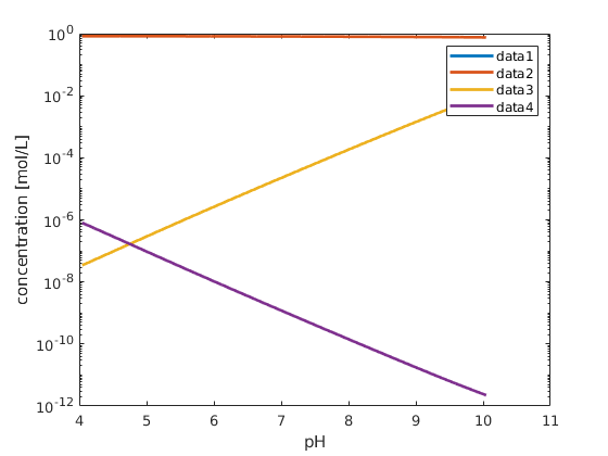
define the inputs¶

here we vary pH from 4 to 10

n = 500;

Na = 1e-2.*ones(n,1);
Cl = 1e-2*ones(n,1);
H2O = ones(n,1);
H = logspace(-4, -10, n)';

userInput = [Na Cl H H2O]*mol/litre;


[state, report, model] = chemmodel.initState(userInput, 'chargeBalance', 'Na');

Computing initial guess...
===============================================================================================================================================================================================================================================================================================
| It # | H2O=H++OH- (cell) | NaCl=Na++Cl- (cell) | >SOH=>SO-+H+ (cell) | >SOH+H+=>SOH2+ (cell) | >SO-+Na+=>SONa (cell) | >SOH2++Cl-=>SOH2Cl (cell) | Conservation of O (cell) | Conservation of H (cell) | Conservation of Na (cell) | Conservation of Cl (cell) | Conservation of >SO (cell) |
===============================================================================================================================================================================================================================================================================================
|    1 | 2.30e+01          | 2.30e+00            | 8.06e+00            | 1.84e+01              | 4.37e+00              | 4.37e+00                  | 6.93e-01                 | 2.08e+00                 | 5.70e+00                  | 5.70e+00                  | 8.70e+00                   |
|    2 |*1.78e-15          | 8.96e+00            | 5.45e+00            | 7.40e+00              | 1.10e+01              | 1.00e+01                  | 1.08e+01                 | 9.74e+00                 | 6.99e-01                  | 6.93e-01                  | 7.77e-01                   |
|    3 |*0.00e+00          | 6.08e+00            | 2.17e+00            | 2.17e+00              | 6.93e+00              | 1.84e+00                  |*8.88e-16                 | 1.03e-03                 | 2.94e-01                  | 2.23e-01                  | 2.92e-01                   |
|    4 |*0.00e+00          | 2.11e+00            | 5.61e-01            | 4.88e-02              | 1.45e+00              | 1.22e+00                  |*0.00e+00                 | 2.39e-05                 | 8.25e-03                  | 8.20e-03                  | 3.98e-02                   |
...

post processing¶

to add the surface potentials and charges to the state structure we must call on functions within ChemicalModel

[state, chemmodel] = chemmodel.updateActivities(state);
[state, chemmodel] = chemmodel.updateChargeBalance(state);
[state, chemmodel] = chemmodel.updateSurfaceCharges(state);
[state, chemmodel] = chemmodel.updateSurfacePotentials(state);
[state, chemmodel] = chemmodel.updateAqueousConcentrations(state);
[state, chemmodel] = chemmodel.updateSurfaceConcentrations(state);

state = changeUnits(state, {'elements', 'species', 'activities'}, mol/litre);

pH = -log10(getProp(chemmodel, state, 'aH+'));

plot the results¶

% plot the charge balance of the system
figure; hold on; box on;
plot(pH, state.chargeBalance,'-k')
xlabel('pH')
ylabel('charge [% of total ion concentration]');

% plot the concentration of elements on the surface
figure; hold on; box on;
plot(pH, state.surfaceConcentrations, 'linewidth',2)
xlabel('pH')
ylabel('concentration [mol/L]');
set(gca, 'yscale', 'log');
legend(chemsys.surfaceConcentrationNames);

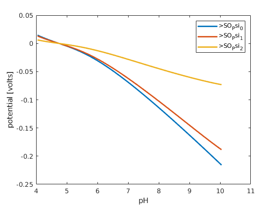
% plot the surface potentials, there are three surfaces in the triple layer
% model
figure; hold on; box on;
plot(pH, state.surfacePotentials, 'linewidth',2)
xlabel('pH')
ylabel('potential [volts]');
legend(chemsys.surfacePotentialNames);

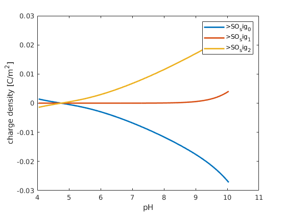
% plot the surface charges, they will sum to zero
figure; hold on; box on;
plot(pH, state.surfaceCharges, 'linewidth',2)
xlabel('pH')
ylabel('charge density [C/m^2]');
legend(chemsys.surfaceChargeNames);

Copyright notice¶

close all;
clear;

add the necessary modeules¶

Generated from injectorProducerArray.m

mrstModule add ad-core ad-props ad-blackoil geochemistry mrst-gui
mrstVerbose off

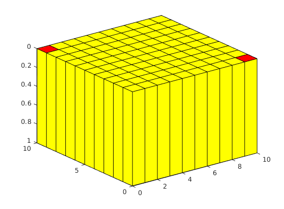
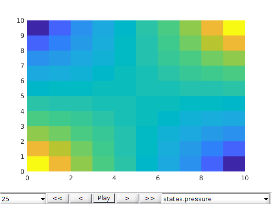
Define the domain¶

here we look at a 2D cartesian grid with 100 cells

sideLength = 10;
G = cartGrid([sideLength, sideLength, 1], [sideLength, sideLength, 1]);
G = computeGeometry(G);
nc = G.cells.num;

% you can view the domain using plotGrid
plotGrid(G), view(3), axis tight
outInd = [G.faces.num-G.cells.num-sideLength+1; G.faces.num-G.cells.num-sideLength^2+sideLength];

% here we plot the faces of a zero dirchlet boundary condition in pressure
plotFaces(G, outInd, 'r');

Define the rock¶

porosity and permeability are the minimum number of parameters for rock

rock.perm = 1*darcy*ones(G.cells.num, 1);
rock.poro = 0.5*ones(G.cells.num, 1);

Define the fluid¶

pRef = 0*barsa;
fluid = initSimpleADIFluid('phases', 'W', 'mu', 1*centi*poise, 'rho', ...
                           1000*kilogram/meter^3, 'c', 1e-10, 'cR', 4e-10, ...
                           'pRef', pRef);

Define the chemistry¶

here we look at a simple tracer chemical system

elements = {'O', 'H', 'Na*','Cl*'};

species = {'H+*', 'OH-', 'Na+', 'H2O*', 'NaCl','Cl-'};

reactions ={'H2O  = H+  + OH- ',      10^-14*mol/litre, ...
            'NaCl = Na+ + Cl-',       10^1*mol/litre};

% instantiate chemical model
chemsys = ChemicalSystem(elements, species, reactions);

chemmodel = ChemicalModel(chemsys);

solve the chemistry for the initial and injected compositions¶

we will be injected a low slainity fluid into a high salinity aquifer. we solve the system so that we can give the total element concentrations within the domain at the initial time, and define the boundary conditions

% initial chemistry
Nai = 1e-1;
Cli = Nai;
Hi = 1e-7;
H2Oi = 1;
initial = [Nai Cli Hi H2Oi]*mol/litre;

% we must repeat the initial chemistry for each cell of the system. This
% can be done by passing a vector to initState, or repmatting the state
% variable produced
[initChemState, initreport]= chemmodel.initState(repmat(initial, nc,1), 'charge', 'Cl');

% the initial state must also contain a pressure field
initChemState.pressure = pRef*ones(nc,1);

% injected chemistry
Naf = 1e-3;
Clf = Naf;
Hf = 1e-10;
H2Of = 1;
injected = [Naf Clf Hf H2Of]*mol/litre;
[injChemState, injreport]= chemmodel.initState(injected, 'charge', 'Cl');

Computing initial guess...
Solving the chemical system with strict charge balance...
Computing initial guess...
Solving the chemical system with strict charge balance...

Define the transport model¶

model = ChemicalTransportModel(G, rock, fluid, chemmodel);

Define the boundary conditions¶

here we have two source cells in the southwest and northeast corners. there are two dirchlet conditions in the northwest and southeast corners allowing for outflow. Defining only neumann boundary conditions will underconstain the pressure solution such that a constant of integration is unknown.

% grab the volume of each cell in the domain
pv = poreVolume(G,rock);

% inject one pore volume into the cells per day.
src                   = [];
src                   = addSource(src, [1; nc], pv(1:2)/day, 'sat', 1);

% define chemistry of the injected fluid
src.elements        = injChemState.elements(end,:);
src.logElements     = injChemState.logElements(end,:);

% specifiy dirchlet conditions for the composition
bc                  = [];
outInd = [G.faces.num-G.cells.num-sideLength+1; G.faces.num-G.cells.num-sideLength^2+sideLength];
bc                  = addBC(bc, outInd, 'pressure', [0; 0]*barsa, 'sat', 1);
bc.elements         = initChemState.elements(end,:);        % will not used if outflow
bc.logElements      = initChemState.logElements(end,:);  % will not used if outflow

Define the time stepping schedule¶

here we define the time stepping schedule. it is recommended to ramp up the size of the time steps gradually

schedule.step.val = [0.01*day*ones(5, 1); 0.1*day*ones(5,1); 1*day*ones(5, 1); 5*day*ones(10, 1)];
schedule.step.control = ones(numel(schedule.step.val), 1);
schedule.control = struct('bc', bc, 'src', src, 'W', []);

Run the simulation¶

[~, states, scheduleReport] = simulateScheduleAD(initChemState, model, schedule);

Solving timestep 01/25:                                   -> 864 Seconds
Solving timestep 02/25: 864 Seconds                       -> 1728 Seconds
Solving timestep 03/25: 1728 Seconds                      -> 2592 Seconds
Solving timestep 04/25: 2592 Seconds                      -> 3456 Seconds
Solving timestep 05/25: 3456 Seconds                      -> 1 Hour, 720 Seconds
Solving timestep 06/25: 1 Hour, 720 Seconds               -> 3 Hours, 2160 Seconds
Solving timestep 07/25: 3 Hours, 2160 Seconds             -> 6 Hours
Solving timestep 08/25: 6 Hours                           -> 8 Hours, 1440 Seconds
...

visualize the simulation¶

plotToolbar(G, states, 'field', 'pressure','startplayback', true)

Copyright notice¶

close all;
clear;

load appropriate modules¶

Generated from solidSystemTransport.m

mrstModule add ad-core ad-props ad-blackoil geochemistry
mrstVerbose off

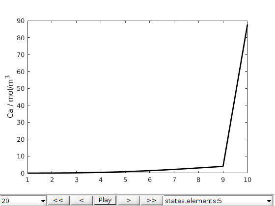
Define the domain¶

simple 1D cartesian domain

G = cartGrid([10, 1, 1], [100, 1, 1]);
G = computeGeometry(G);
nc = G.cells.num;

Define the rock¶

rock.perm = 1*darcy*ones(G.cells.num, 1);
rock.poro = 0.3*ones(G.cells.num, 1);

Define the fluid¶

pRef = 0*barsa;
fluid = initSimpleADIFluid('phases', 'W', 'mu', 1*centi*poise, 'rho', ...
                           1000*kilogram/meter^3, 'c', 1e-10, 'cR', 4e-10, ...
                           'pRef', pRef);

Define the chemistry¶

here we have the carbonate system with calcite precipitation

elements = {'O', 'H', 'Na*', 'Cl*', 'Ca*', 'C*'};

species = {'H+*', 'OH-', 'Na+', 'Cl-', 'NaOH', 'H2O*',...
             'Ca+2', 'CO3-2', 'HCO3-', 'CO2',...
             'CaCO3(s)'};

reactions ={'H2O  = H+  + OH- '       , 10^-14*mol/litre, ...
            'NaOH = Na+ + OH-'        , 10^10*mol/litre, ...
            'CaCO3(s) = CO3-2 + Ca+2' , 10^-8.48*(mol/litre)^2, ...
            'CO3-2 + H+ = HCO3-'      , 10^10.329/(mol/litre), ...
            'CO3-2 + 2*H+ = CO2 + H2O', 10^16.681/(mol/litre)};

chemsys = ChemicalSystem(elements, species, reactions);

% print the chemical model to the screen
chemsys.printChemicalSystem;

% instantiate chemical model
chemmodel = ChemicalModel(chemsys);

% initial chemistry
Nai = 1e-1;
Cli = Nai;
Cai = 1e-2;
Ci = 1e-3;
Hi = 1e-9;
H2Oi = 1;

inputConstraints = [Nai Cli Cai Ci Hi H2Oi]*mol/litre;
[initchemstate, initreport]= chemmodel.initState(repmat(inputConstraints, nc,1), 'charge', 'Cl');

% injected chemistry, we are injecting less Ca into the system
Naf = 1e-1;
Clf = Naf;
Caf = 1e-3;
Cf = 1e-3;
Hf = 1e-9;
H2Of = 1;

inputConstraints = [Naf Clf Caf Cf Hf H2Of]*mol/litre;
[injchemstate, injreport] = chemmodel.initState(inputConstraints, 'charge', 'Cl');

====================================================================================================================================
|Equations           |       H+|      OH-|      Na+|      Cl-|     NaOH|      H2O|     Ca+2|    CO3-2|    HCO3-|      CO2| CaCO3(s)|
====================================================================================================================================
|sum(O)              |        0|        1|        0|        0|        1|        1|        0|        3|        3|        2|        3|
|sum(H)              |        1|        1|        0|        0|        1|        2|        0|        0|        1|        0|        0|
|sum(Na)             |        0|        0|        1|        0|        1|        0|        0|        0|        0|        0|        0|
|sum(Cl)             |        0|        0|        0|        1|        0|        0|        0|        0|        0|        0|        0|
...

Define the initial state¶

initState = initchemstate;
initState.pressure = pRef*ones(nc,1);

instantiate the transport model¶

model = ChemicalTransportModel(G, rock, fluid, chemmodel);

Define the boundary conditions¶

% define the initial and injected fluid composition states
injfluidpart = injchemstate.elements;
initfluidpart = initchemstate.elements(end,:);

% sxtract the pore volumes from the domain
pv = poreVolume(G,rock);

% define source term at cell 1 for inflow boundary condition
src = [];
src = addSource(src, 1, pv(1)/day, 'sat', 1);

% give the fluid concentration at the inlet
src.elements    = injfluidpart;
src.logElements = log(injfluidpart);

% give dirchlet boundary condition at outlet
bc             = [];
bc             = pside(bc, G, 'east', 0*barsa, 'sat', 1);
bc.elements    = initfluidpart;        % (will not be used if outflow)
bc.logElements = log(initfluidpart);  % (will not be used if outflow)

Define the schedule¶

it is recommended to ramp up the time steps

% ten time steps of 0.01 days followed by 100 steps of 1 day
schedule.step.val     = [0.01*day*ones(10, 1); 1*day*ones(10, 1);];
schedule.step.control = ones(numel(schedule.step.val), 1);
schedule.control      = struct('bc', bc, 'src', src, 'W', []);

Run the simulation¶

[~, states, scheduleReport] = simulateScheduleAD(initState, model, schedule);
mrstModule add mrst-gui

plotToolbar(G, states, 'field', 'elements:5', 'plot1d', true,'startplayback',true)
ylabel('Ca / mol/m^3')

Solving timestep 01/20:                                   -> 864 Seconds
Solving timestep 02/20: 864 Seconds                       -> 1728 Seconds
Solving timestep 03/20: 1728 Seconds                      -> 2592 Seconds
Solving timestep 04/20: 2592 Seconds                      -> 3456 Seconds
Solving timestep 05/20: 3456 Seconds                      -> 1 Hour, 720 Seconds
Solving timestep 06/20: 1 Hour, 720 Seconds               -> 1 Hour, 1584 Seconds
Solving timestep 07/20: 1 Hour, 1584 Seconds              -> 1 Hour, 2448 Seconds
Solving timestep 08/20: 1 Hour, 2448 Seconds              -> 1 Hour, 3312 Seconds
...

Copyright notice¶

close all;
clear;

mrstModule add ad-core ad-props ad-blackoil geochemistry

mrstVerbose off

Define the grid¶

Generated from surfaceSystemTransport.m

here we define a 1D domain with 10 cells, each a meter in length

G = cartGrid([10, 1, 1], [10, 1, 1]);
G = computeGeometry(G);
nc = G.cells.num;

Define the rock¶

rock.perm = 1*darcy*ones(G.cells.num, 1);
rock.poro = ones(G.cells.num, 1);

Define the fluid¶

pRef = 0*barsa;
fluid = initSimpleADIFluid('phases', 'W', 'mu', 1*centi*poise, 'rho', ...
                           1000*kilogram/meter^3, 'c', 1e-10, 'cR', 4e-10, ...
                           'pRef', pRef);

Define the chemistry¶

the chemical system include the speciation of NaCl and H2O, as well as a reactive silica surface which can have a negative or neutral surface

elements = {'O', 'H', 'Na*','Cl*'};

species = {'H+*', 'OH-', 'Na+', 'H2O*', '>SiO-', '>SiOH', 'NaCl','Cl-'};

reactions ={'H2O  = H+  + OH- ',      10^-14*mol/litre, ...
            'NaCl = Na+ + Cl-',       10^1*mol/litre,...
            '>SiOH = >SiO- + H+',     10^-8*mol/litre};

geometry = [2*site/(nano*meter)^2 50e-3*meter^2/(gram) 5e3*gram/litre];
sioInfo = {geometry, 'tlm', [1 1e3], '>SiO-', [-1 0 0], '>SiOH', [0 0 0]};

surfaces = {'>SiO', sioInfo};

% instantiate chemical model object
chemsys = ChemicalSystem(elements, species, reactions, 'surf', surfaces);

% print the chemical model to the screen
chemsys.printChemicalSystem;

chemmodel = ChemicalModel(chemsys);

================================================================================================================================================================
|Equations      |          H+|         OH-|         Na+|         H2O|       >SiO-|       >SiOH|        NaCl|         Cl-| >SiO_ePsi_0| >SiO_ePsi_1| >SiO_ePsi_2|
================================================================================================================================================================
|sum(O)         |           0|           1|           0|           1|           0|           0|           0|           0|           0|           0|           0|
|sum(H)         |           1|           1|           0|           2|           0|           1|           0|           0|           0|           0|           0|
|sum(Na)        |           0|           0|           1|           0|           0|           0|           1|           0|           0|           0|           0|
|sum(Cl)        |           0|           0|           0|           0|           0|           0|           1|           1|           0|           0|           0|
...

solve for the initial state¶

the column is originally saturated with a basic solution, an acidic solution is injected on the left boundary

% initial chemistry
Nai = 1e-3;
Cli = Nai;
Hi = 1e-9;
H2Oi = 1;

inputConstraints = [Nai Cli Hi H2Oi]*mol/litre;
[initchemstate, initreport]= chemmodel.initState(repmat(inputConstraints, nc,1), 'charge', 'Cl');

initState = initchemstate;
initState.pressure = pRef*ones(nc,1);

% injected chemistry
Naf = 1e-1;
Clf = Nai;
Hf = 1e-9;
H2Of = 1;

inputConstraints = [Naf Clf Hf H2Of]*mol/litre;
[injchemstate, injreport] = chemmodel.initState(inputConstraints, 'charge', 'Cl');

Computing initial guess...
Solving the chemical system with strict charge balance...
Computing initial guess...
Solving the chemical system with strict charge balance...

Define the transport model¶

model = ChemicalTransportModel(G, rock, fluid, chemmodel);

Define the boundary conditions¶

here we specify a dirchlet boundary condition for pressure on the right hand side, and a constant flux on the left. The total element concentration at the boundaries must be provided.

% use model.fluidMat to pull the fluid concentrations from the injected
% state
injfluidpart  = injchemstate.species*model.fluidMat';
initfluidpart = initchemstate.species(end,:)*model.fluidMat';

pv = poreVolume(G,rock);

% define source term at cell 1 for inflow boundary condition
src = [];
src = addSource(src, 1, pv(1)/day, 'sat', 1);

% give the fluid concentration at the inlet
src.elements = injfluidpart;
src.logElements = log(injfluidpart);

% give dirchlet boundary condition at outlet
bc             = [];
bc             = pside(bc, G, 'east', 0*barsa, 'sat', 1);
bc.elements    = initfluidpart;        % (will not be used if outflow)
bc.logElements = log(initfluidpart);  % (will not be used if outflow)

Define the schedule¶

it is recommened to ramp up the time stepping

% ten time steps of 0.01 days followed by 100 steps of 1 day
schedule.step.val     = [0.01*day*ones(10, 1); 0.1*day*ones(10, 1); 1*day*ones(10, 1);];
schedule.step.control = ones(numel(schedule.step.val), 1);
schedule.control      = struct('bc', bc, 'src', src, 'W', []);

Run the simulation¶

[~, states, scheduleReport] = simulateScheduleAD(initState, model, schedule);

Solving timestep 01/30:                                   -> 864 Seconds
Solving timestep 02/30: 864 Seconds                       -> 1728 Seconds
Solving timestep 03/30: 1728 Seconds                      -> 2592 Seconds
Solving timestep 04/30: 2592 Seconds                      -> 3456 Seconds
Solving timestep 05/30: 3456 Seconds                      -> 1 Hour, 720 Seconds
Solving timestep 06/30: 1 Hour, 720 Seconds               -> 1 Hour, 1584 Seconds
Solving timestep 07/30: 1 Hour, 1584 Seconds              -> 1 Hour, 2448 Seconds
Solving timestep 08/30: 1 Hour, 2448 Seconds              -> 1 Hour, 3312 Seconds
...

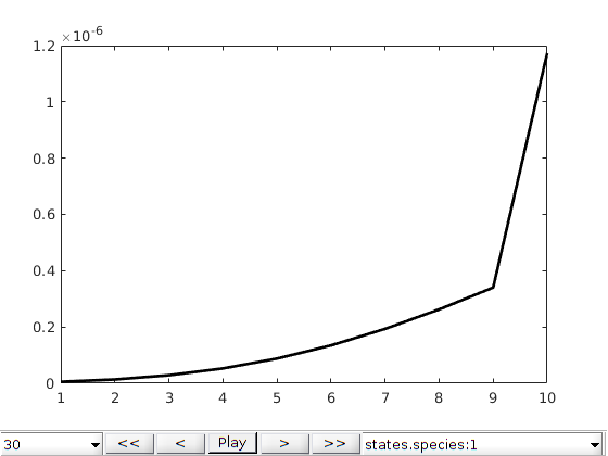
visualize the simulation¶

mrstModule add mrst-gui
plotToolbar(G, states, 'field', 'species:1','startplayback', true, 'plot1D', true)

geochemistry: Surface geochemistry¶

4. In startup_user.m add the line¶

mrstPath(‘register’, ‘geochemistry’, ‘path/to/repo/matlab-geochemistry’)¶

mrstModule add geochemistry ad-core¶

Examples¶

load adi and geochemistry module¶

define the chemical model¶

solve the chemical system given inputs¶

Copyright notice¶

load adi and geochemistry module¶

generate chemical system¶

define input parameters¶

solve the chemical system¶

calculate auxillary information¶

data from Goldberg¶

plot the results¶

Copyright notice¶

add adi and geochemistry modules¶

instantiate the chemical model¶

specify inputs¶

solve the chemical system¶

process the data¶

plot the results¶

Copyright notice¶

load adi and geochemistry module¶

instantiate the chemical system¶

specify inputs¶

solve chemical system given inputs¶

process data¶

plot the results¶

Copyright notice¶

Add geochemistry and automatic differentiation modules¶

instantiate chemical model¶

define input values¶

solve the chemical system¶

calculate acitivities and charge balance¶

visualize the results¶

Copyright notice¶

load ad and geochemistry modules¶

generate chemical system object¶

define the input¶

solve the chemical system¶

process the data¶

plot the results¶

Copyright notice¶

load adi and geochemistry module¶

generate chemical system¶

define the inputs¶

post processing¶

plot the results¶

Copyright notice¶

add the necessary modeules¶

Define the domain¶

Define the rock¶

Define the fluid¶

Define the chemistry¶

solve the chemistry for the initial and injected compositions¶

Define the transport model¶

Define the boundary conditions¶

Define the time stepping schedule¶

Run the simulation¶

visualize the simulation¶

Copyright notice¶

load appropriate modules¶

Define the domain¶

Define the rock¶

Define the fluid¶

Define the chemistry¶

Define the initial state¶

instantiate the transport model¶

Define the boundary conditions¶

Define the schedule¶

Run the simulation¶

Copyright notice¶

Define the grid¶

Define the rock¶

Define the fluid¶

Define the chemistry¶

solve for the initial state¶

Define the transport model¶

`geochemistry`: Surface geochemistry¶