`msfvm`: Multiscale Finite-Volume method for pressure¶

Implementation of the Multiscale Finite Volume (MsFV) solver for structured and unstructured grids.

The MsFV solver requires a dual-primal coarse partition and relies on the solution of reduced flow problems along dual edges/faces for localization. Hence, the method may not work well for grids with complex grids and/or cases with very strong media contrasts. See the msrsb module for a more robust and versatile method.

Utilities¶

Contents¶

MSFVM

Files: createPermutationMatrix - Create permutation matrices for the coarse orderings in the MsFV find_clusters - Undocumented Utility Function findCenter - indices of blocks in the current cell mldivide_update - A,b linear system partitionUIdual - Create coarse dual partition/grid plotDual - Plot an implicitly defined dual grid for the multiscale finite volume method reportError - Simple error helper for MsFV examples solveMSFV_TPFA_Incomp - Solve incompressible flow problem (flux/pressures) using a multiscale

plotDual¶

Plot an implicitly defined dual grid for the multiscale finite volume method

Synopsis:

plotDual(G, dual)

Parameters:	G – Grid structure dual – Dual grid as defined by for example partitionUIdual.

createPermutationMatrix(A, dual, CG, varargin)¶

Create permutation matrices for the coarse orderings in the MsFV

Synopsis:

Creates permutation matrices

Description:

The MsFV is dependent on reordering the system matrices. This takes a dual grid and coarse grid and uses them to create permutation matrices for both primal and inner, edge… orderings

Keyword Arguments:
Parameters:	-- Not in use (A) – -- Dual coarse grid such as defined by dualPartition (dual) – -- Coarse grid as defined by for example partitionUI (CG) –
	wells – well data structure SpeedUp – Alternate formulation of the method requires alternate ordering matrices
Returns:	CG – Coarse grid with updated partition structure to account for wells dual – Updated dual grid with permutation matrices

Note

This function is meant for encapsulation within the MSFVM solver, and is subject to change

findCenter(cg, center, blockInd)¶: indices of blocks in the current cell blockInd = find(cg.partition == coarseindex); find the centroids

find_clusters(varargin)¶: Undocumented Utility Function

mldivide_update(A, b, x_old, targets, complist)¶: A,b linear system A_old, b_old old linear system x_old old solution vector targets, list of cells which should be updated (linear subsystems containing one of these cells must be updated) complist as defined by components(A) A should have the same graph, but not the same values as A_old

partitionUIdual(CG, blockSizes)¶

Create coarse dual partition/grid

Synopsis:

Create coarse dual partition/grid using logical partitioning

DESCRIPTION:

Parameters:	-- Coarse grid as defined by partitionUI (CG) – -- block sizes for partitionUI (blockSizes) –
Returns:	dual – Categorization of the nodes

Note

Use dualPartition for non-Cartesian grids or grids with erosion

reportError(reference, ms)¶: Simple error helper for MsFV examples

solveMSFV_TPFA_Incomp(state, G, CG, T, fluid, varargin)¶

Solve incompressible flow problem (flux/pressures) using a multiscale finite volume method.

SYNOPSIS: state = solveMSFV_TPFA_Incomp(state, G, CG, T, fluid) state = solveMSFV_TPFA_Incomp(state, G, CG, T, fluid, ‘pn1’, pv1, …)

DESCRIPTION: This function uses a operator formulation of the multiscale finite volume method to solve a single phase flow problem. The method works on fully unstructured grids, as long as the coarse grids are successfully created.

REQUIRED PARAMTERS:

state - reservoir and well solution structure as defined by

‘initResSol’, ‘initWellSol’ or a previous call to ‘incompTPFA’.

G, T - Grid and half-transmissibilities as computed by the function

‘computeTrans’.

fluid - Fluid object as defined by function ‘initSimpleFluid’.

OPTIONAL PARAMETERS:

wells - Well structure as defined by function ‘addWell’. May be empty

(i.e., W = struct([])) which is interpreted as a model without any wells.

bc - Boundary condition structure as defined by function ‘addBC’.

This structure accounts for all external boundary conditions to the reservoir flow. May be empty (i.e., bc = struct([])) which is interpreted as all external no-flow (homogeneous Neumann) conditions.

src - Explicit source contributions as defined by function

‘addSource’. May be empty (i.e., src = struct([])) which is interpreted as a reservoir model without explicit sources.

LinSolve - Handle to linear system solver software which will be

used to solve the linear equation sets. Assumed to support the syntax

x = LinSolve(A, b)

in order to solve a system Ax=b of linear equations. Should be capable of solving for a matrix rhs. Default value: LinSolve = @mldivide (backslash).

Dual - A dual grid. Will be created if not already defined.

Verbose - Controls the amount of output. Default value from

mrstVerbose global

Reconstruct - Determines if a conservative flux field will be

constructed after initial pressure solution.

Discretization - Will select the type of stencil used for approximating

the pressure equations. Currently only TPFA.

Iterations - The number of iterations performed. With subiterations

and a smoother, the total will be subiter*iter.

Subiterations - When using smoothers, this gives the number of

smoothing steps.

Tolerance - Termination criterion for the iterative variants.

CoarseDims - For logical partitioning scheme, the coarse dimensions

must be specified.

Restart - The number of steps before GMRES restarts.

Iterator - GMRES, DAS or DMS. Selects the iteration type.

Omega - Relaxation paramter for the smoothers

Scheme - The scheme used for partitioning the dual grid. Only

used when no dual grid is supplied.

DoSolve - Will the linear systems be solved or just outputted?

Speedup - Alternative formulation of the method leads to great

speed improvements in 3D, but may have different error values and is in general more sensitive to grid errors

Update - If a state from a previous multiscale iteration is

provided, should operators be regenerated?

DynamicUpdate - Update pressure basis functions adaptively. Requires

dfs search implemented as components

RETURNS:

state - Update reservoir and well solution structure with new values

for the fields:

pressure – Pressure values for all cells in the

discretised reservoir model, ‘G’.

pressure_reconstructed – Pressure values which gives

conservative flux

pressurecoarse – Coarse pressure used for solution

facePressure –

Pressure values for all interfaces in the discretised reservoir model, ‘G’.

time – Timing values for benchmarking

flux – Flux across global interfaces corresponding to

the rows of ‘G.faces.neighbors’.

M_ee,A_ii– Relevant matrices for debugging

DG – Dual grid used

A – System matrix. Only returned if specifically

requested by setting option ‘MatrixOutput’.

wellSol – Well solution structure array, one element for

each well in the model, with new values for the fields:

flux – Perforation fluxes through all

perforations for corresponding well. The fluxes are interpreted as injection fluxes, meaning positive values correspond to injection into reservoir while negative values mean production/extraction out of reservoir.

pressure – Well bottom-hole pressure.

NOTE:

The multiscale solver is based on function incompTPFA.

SEE ALSO:

incompTPFA.

Examples¶

MsFV example on PEBI grid¶

Generated from PEBImsfvExample.m

This example demonstrates the use of the MsFV method on unstructured grids using a PEBI grid. This grid is unstructured in ij-space. We start by loading the required modules and a stored binary file that includes the grids. If the stored binary file is not found, it is downloaded from the Internet (approximately 15 MB download)

mrstModule add msfvm mrst-gui mex agglom coarsegrid incomp

if ~exist('pebi_with_dual.mat', 'file')
    disp('Did not find grid, downloading (~15.0 MB)')
    msfvmdir = fullfile(mrstPath('query', 'msfvm'), 'examples');
    unzip('http://www.sintef.no/project/MRST/pebi_with_dual.mat.zip', msfvmdir)
end

load pebi_with_dual

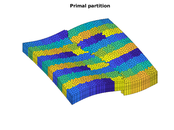
Plot the coarse grids (dual and primal)¶

v = [150, 70];

clf; plotCellData(G, mod(CG.partition,17), 'edgecolor', 'k', 'edgea', .5);
title('Primal partition')
view(v), axis tight off;

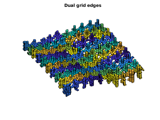
figure;
plotCellData(G, mod(CG.partition,17), DG.lineedge, 'EdgeColor', 'w')
title('Dual grid edges')
view(v), axis tight off;

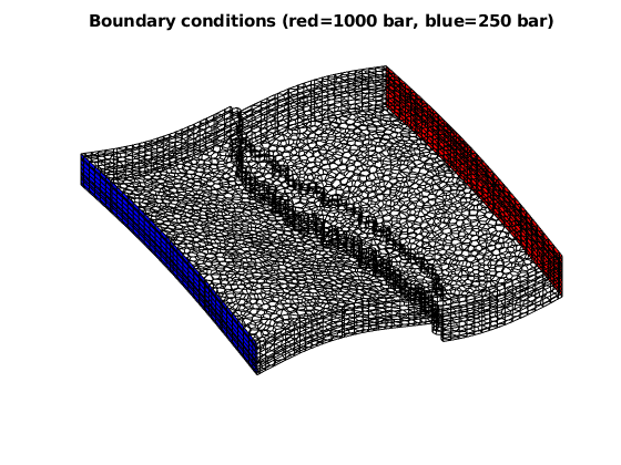
Set up boundary conditions and fluid¶

bc = [];
d  = abs(G.faces.centroids(:,1) - max(G.faces.centroids(:,1)));
es = find (d < 1e6*eps);

d  = abs(G.faces.centroids(:,1) - min(G.faces.centroids(:,1)));
ws = find (d < 1e6*eps);

bc = addBC(bc, ws, 'pressure', 1000*barsa());
bc = addBC(bc, es, 'pressure', 250*barsa());
fluid        = initSingleFluid('mu' ,    1*centi*poise     , ...
                               'rho', 1014*kilogram/meter^3);
clf; plotGrid(G, 'facea', 0)
plotFaces(G, ws, 'FaceColor', 'red')
plotFaces(G, es, 'FaceColor', 'blue')
title('Boundary conditions (red=1000 bar, blue=250 bar)')
view(v)
axis tight off

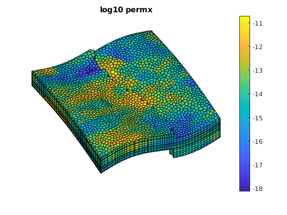
Set up the permeability¶

The values here can be changed to solve either a homogenous permeability field or two variants of the SPE10 mapped onto the grid using nearest neighbor interpolation. The default is the Tarbert layers which is inbetween the homogenous permeability and the Ness layers in terms of difficulty.

gridtype = 'spe10';
% Uncomment to take uniform permeability instead
% gridtype = 'uniform';

% Take the Tarbert layers
offset = 0;
% Uncomment to take Ness layers instead
% offset = 35;

switch lower(gridtype)
    case 'uniform'
        rock.perm = 100*milli*darcy*ones(G.cells.num,1);
        rock.poro = ones(G.cells.num, 1);
    case 'spe10'
        % We have 12 layers in the model
        Nz = 12;
        mrstModule add spe10 mex

        [Gspe, W, rockspe] = getSPE10setup((1:Nz) + offset);
        % Normalize coordinates to make it easier to map the values
        normalize = @(x) bsxfun(@rdivide, x, max(x));
        c = normalize(Gspe.cells.centroids);
        rock.perm = zeros(G.cells.num, 3);
        for i = 1:3
            % Interpolate the permeability using nearest neighbor
            % interpolation
            pperm = TriScatteredInterp(c, rockspe.perm(:, i) , 'nearest');
            rock.perm(:, i) = pperm(normalize(G.cells.centroids));
        end
    otherwise
        error('Unknown case')
end

sol = initState(G, [], 0, 1);
T = computeTrans(G, rock);

% Plot the permeability
figure(1);
clf;
plotCellData(G, log10(rock.perm(:, 1)));
axis tight off; view(v); colorbar;
title('log10 permx')

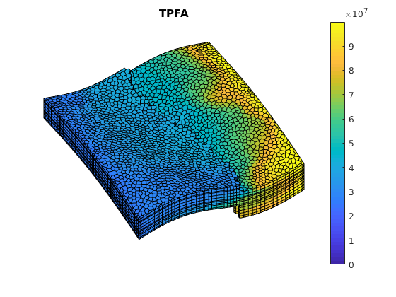
Solve the reference solution¶

Standard two point scheme

disp 'Solving TPFA reference'
tic;
solRef = incompTPFA(sol, G, T, fluid, 'bc', bc, 'MatrixOutput', true);
toc;

Solving TPFA reference
Elapsed time is 0.180890 seconds.

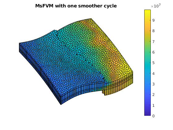
Set up msfv solver and solve¶

We call the solver twice to both obtain the uniterated solution as well as a solution where a single smoother cycle has been applied (5 steps with block gauss-seidel / DMS).

solvems = @(iterator, iterations, smoother, subiterations, omega, verb, restart) ...
          solveMSFV_TPFA_Incomp(sol, G, CG, T, fluid, 'Dual', DG, 'Reconstruct', true, 'bc', bc, 'Verbose', verb, 'SpeedUp', true,...
          'Iterator', iterator, 'Iterations', iterations, 'Smoother', smoother, 'Subiterations', subiterations, 'Omega', omega, 'Restart', restart);

disp 'Solving MSFVM'
[sol_msfv] = solvems('msfvm', 1, 'dms', 5, 1, true, 0);



disp 'Solving MSFVM'
[sol_msfv_0] = solvems('msfvm', 0, 'dms', 0, 1, true, 0);

Solving MSFVM
Warning: solveMSFV_TPFA_Incomp is DEPRECATED! Please use incompMultiscale from
the "msrsb" module instead.
Decoupling edge systems...
Generating dual partition...
Elapsed time is 0.000035 seconds.
Generating permutation matrix...
Generating operators...
...

Plot all solutions in seperate plots and the error¶

figure(1);
clf;
plotCellData(G, solRef.pressure);
axis tight off; view(v); colorbar;
set(gca, 'CLim', [0, max(solRef.pressure)]);
title('TPFA')

figure(2);
clf;
plotCellData(G, sol_msfv.pressure);
axis tight off; view(v); colorbar;
    title('MsFVM with one smoother cycle')
% Use same axis scaling as the TPFA solution
set(gca, 'CLim', [0, max(solRef.pressure)]);

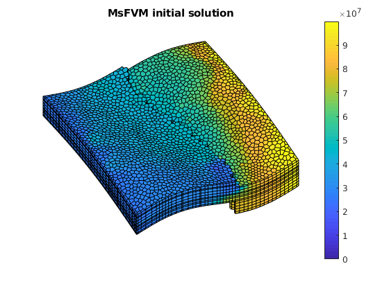
figure(3);
clf;
plotCellData(G, sol_msfv_0.pressure);
axis tight off; view(v); colorbar;
    title('MsFVM initial solution')
% Use same axis scaling as the TPFA solution
set(gca, 'CLim', [0, max(solRef.pressure)]);


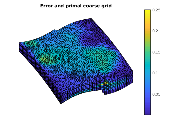
figure(4);
clf;
err = abs(sol_msfv.pressure - solRef.pressure)./solRef.pressure;
plotCellData(G, err);
outlineCoarseGrid(G, CG.partition);
axis tight off; view(v); colorbar;
title('Error and primal coarse grid')

Example demonstrating the effects of aspect ratios and contrast on msfvm¶

Generated from contrastAndAspectError.m

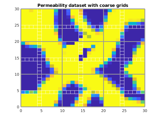
The Multiscale Finite Volume method is based on approximating boundary conditions using lower dimensional solutions. This approach is local in nature and gives good results for relatively smooth heterogeneties, but is sensitive to high contrast, high aspect ratios. In this example we will show how a single dataset, realized with different levels of contrast and aspect ratios can demonstrate the limits of the method. Note that this example is intentionally difficult, placing the dual grid boundary over a high contrast region. This makes the boundary conditions resulting from the lower dimensional numerical solution a poor approximation of the global field, giving both a degenerate coarse scale operator and a poor prolongation operator if the contrast is large.

mrstModule add mrst-gui coarsegrid msfvm incomp

G = cartGrid([30 30]);
G = computeGeometry(G);

Cdims = [3,3];
p = partitionUI(G, Cdims);

CG = generateCoarseGrid(G, p);
CG = coarsenGeometry(CG);
DG = partitionUIdual(CG, Cdims);

% Read in an image for permeability
im = double(imread('perm_mono.gif'))';

clf;
plotCellData(G, im(:), 'EdgeColor', 'none')
view(0, 90)
axis tight
title('Permeability dataset with coarse grids')

% Plot dual coarse grid
plotGrid(G, DG.ee, 'FaceColor', 'none', 'EdgeColor', 'w')
% Plot primal coarse grid
outlineCoarseGrid(G, p, [1 1 1].*.6)

Define a wide range of numerical experiments¶

We define a matrix of different contrasts and aspect ratios to get data to show how the solution quality varies. At each combination, we store the error

$e_{ms} = \frac{\| p_{ms} - p_{ref} \|_2}{\|p_{ref}\|_2}$

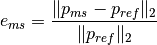
for further use with plotting.

cexp = 0:.5:8;
contrasts = 10.^-(cexp);
aspects = [1 5 10 25 100];
nc = numel(contrasts);
na = numel(aspects);


solutions = cell(nc, na);
errors = nan(nc, na);

normerr = @(ms, ref, k) norm(ref - ms, k)/norm(ref, k);

for i = 1:nc
    for j = 1:na
        aspect = aspects(j);
        % Set up grid with aspect ratio
        G = cartGrid([30 30], [30*aspect, 30]*meter);
        G = computeGeometry(G);

        % Scale permeability mapping with contrast ratio
        hi = 1*darcy;
        lo = contrasts(i)*darcy;

        im = double(imread('perm_mono.gif'))';
        im = im./max(im(:));

        im = hi*im + lo;
        rock.perm = double(im(:));

        T = computeTrans(G, rock);

        % Set up linear flow boundary conditions
        bc = [];
        d  = abs(G.faces.centroids(:,1) - max(G.faces.centroids(:,1)));
        es = find (d < 1e6*eps);

        d  = abs(G.faces.centroids(:,1) - min(G.faces.centroids(:,1)));
        ws = find (d < 1e6*eps);

        bc = addBC(bc, ws, 'pressure', 1);
        bc = addBC(bc, es, 'pressure', 0);

        % Trivial fluid
        fluid        = initSingleFluid('mu' ,    1*centi*poise     , ...
                                       'rho', 1014*kilogram/meter^3);

        sol = initResSol(G, 0);
        % Solve multiscale
        ms = solveMSFV_TPFA_Incomp(sol, G, CG, T, fluid, 'Dual', DG, 'Reconstruct', true, 'bc', bc);
        % Solve TPFA reference
        ref = incompTPFA(sol, G, T, fluid, 'bc', bc);
        % Store the error and solutions
        errors(i, j) = normerr(ref.pressure, ms.pressure, 2);
        solutions{i, j} = struct('ms', ms.pressure, 'ref', ref.pressure);
    end
end

Warning: solveMSFV_TPFA_Incomp is DEPRECATED! Please use incompMultiscale from
the "msrsb" module instead.
Warning: solveMSFV_TPFA_Incomp is DEPRECATED! Please use incompMultiscale from
the "msrsb" module instead.
Warning: solveMSFV_TPFA_Incomp is DEPRECATED! Please use incompMultiscale from
the "msrsb" module instead.
Warning: solveMSFV_TPFA_Incomp is DEPRECATED! Please use incompMultiscale from
the "msrsb" module instead.
...

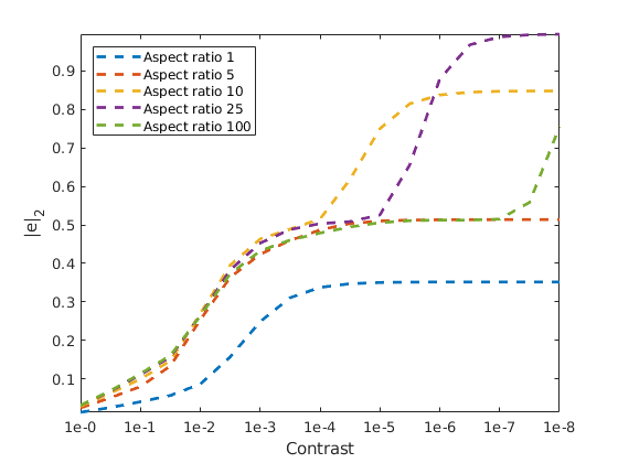
Plot the numerical results¶

We plot the error as a function of the increasing contrast for the different aspect ratios. As we can see, increasing either will make the problem more challenging.

clf

axis tight
plot(cexp, errors, '--', 'LineWidth', 2)
ylim([0 3])
legend(arrayfun(@(x) sprintf('Aspect ratio %d', x), aspects, 'unif', false), 'location', 'northwest')
xlabel('Contrast')
ylabel('|e|_2')


tickx = cexp(1:2:end);

set(gca, 'XTick', tickx, 'XTickLabel', arrayfun(@(x) sprintf('1e-%1.1g', x), tickx, 'unif', false));
axis tight

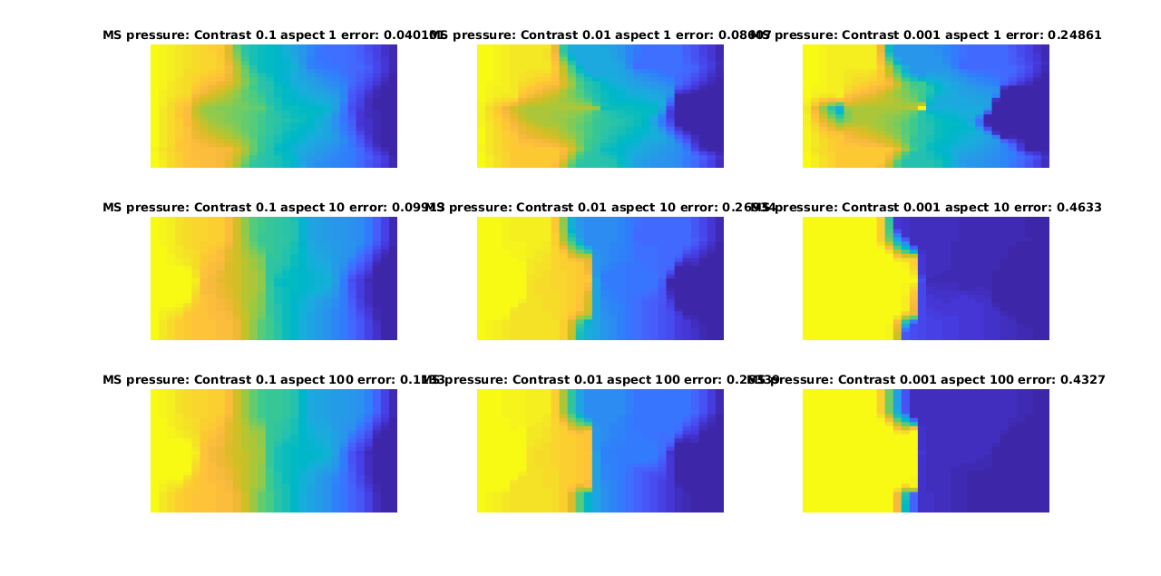
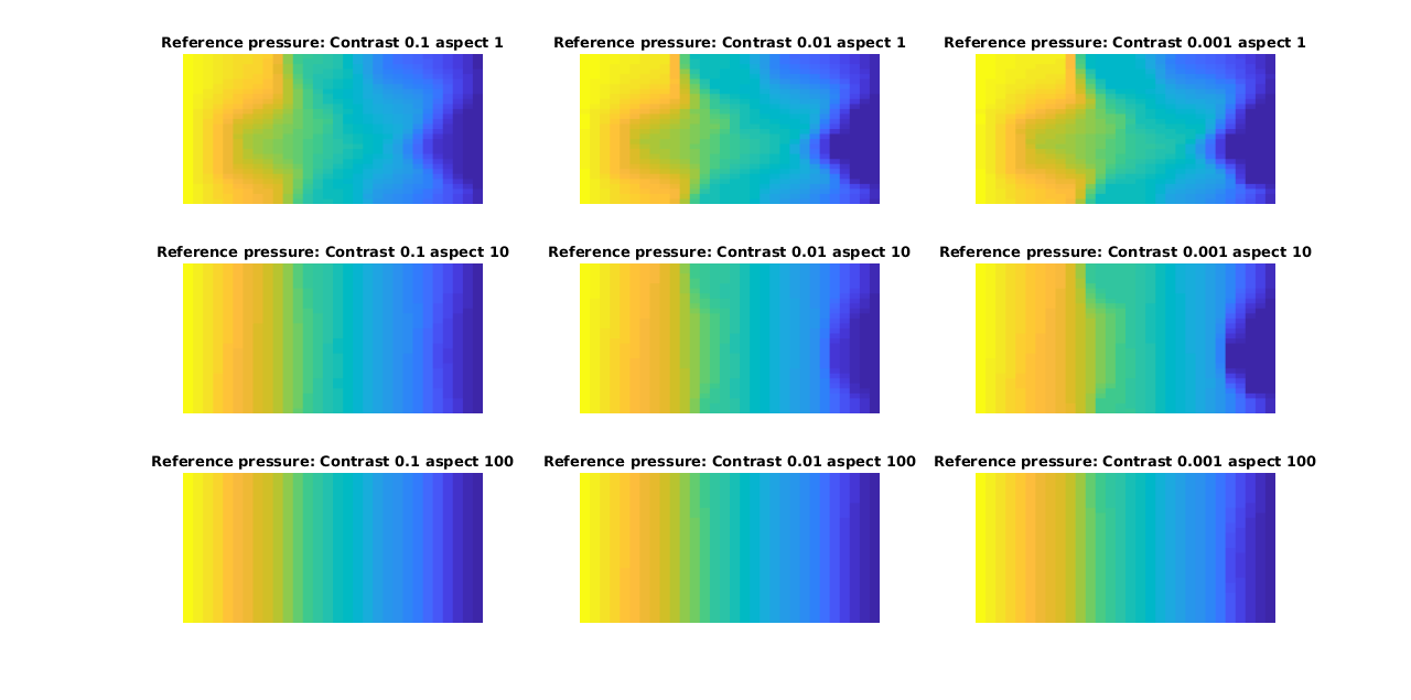
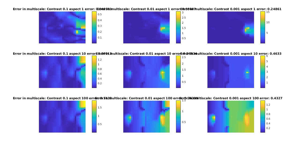
Plot the pressures¶

We plot a subset of the solutions for both multiscale and reference, with the error as as seperate plot. Note that this forms a matrix of plots, where going from left to right along the rows or down the columns increases the error.

close all

h1 = figure('units','normalized','outerposition',[.5 .5 .5 .5]);
h2 = figure('units','normalized','outerposition',[.5 .5 .5 .5]);
h3 = figure('units','normalized','outerposition',[.5 .5 .5 .5]);

% csubs = 1:8:nc;
csubs = [3 5 7];
asubs = 1:2:na;

for i = 1:numel(csubs)
    for j = 1:numel(asubs)
        ci = csubs(i);
        aj = asubs(j);

        ms = solutions{ci, aj}.ms;
        ref = solutions{ci, aj}.ref;

        % Plot multiscale pressure
        set(0, 'CurrentFigure', h1);
        subplot(numel(csubs), numel(asubs), i + (j-1)*numel(csubs))
        plotCellData(G, ms, 'EdgeColor', 'none')
        axis tight off
        title(['MS pressure: Contrast ', num2str(contrasts(ci)), ' aspect ', num2str(aspects(aj)), ' error: ', num2str(errors(ci, aj))])

        caxis([min(ref), max(ref)])

        set(0, 'CurrentFigure', h2);
        subplot(numel(csubs), numel(asubs), i + (j-1)*numel(csubs))
        plotCellData(G, ref, 'EdgeColor', 'none')
        axis tight off
        title(['Reference pressure: Contrast ', num2str(contrasts(ci)), ' aspect ', num2str(aspects(aj))])

        set(0, 'CurrentFigure', h3);
        subplot(numel(csubs), numel(asubs), i + (j-1)*numel(csubs))
        plotCellData(G, abs(ms - ref)./ref, 'EdgeColor', 'none')
        axis tight off
        colorbar
        title(['Error in multiscale: Contrast ', num2str(contrasts(ci)), ' aspect ', num2str(aspects(aj)), ' error: ', num2str(errors(ci, aj))])
    end
end

Example demonstrating Multiscale Finite Volume Solver over a fault for a corner point grid.¶

Generated from faultMSFVExample.m

This is an example demonstrating the MsFV solver on a faulted grid. The coarse dual grid should be provided in the file fault_dual.mat and was produced by an inhouse algorithm.

Load the modules required for the example¶

mrstModule add coarsegrid msfvm incomp

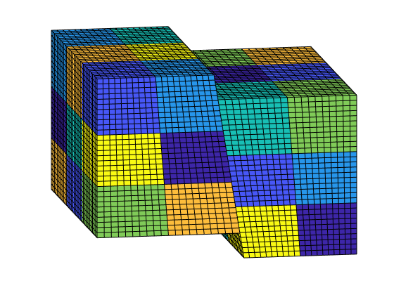
Define grid¶

We define a fine grid of a Cartesian block divided by a sloping fault, with skewed pillars via the GRDECL format. A coarse grid with block size of

is used.

nx = 40; ny = 30; nz = 31;
Nx = 4; Ny = 3; Nz = 3;

% Create grid using deck
grdecl = oneSlopingFault([nx, ny, nz], 5);
G      = processGRDECL(grdecl, 'Verbose', false); clear grdecl;
% Add geometry information
G      = computeGeometry(G);

Generate the coarse grid¶

We process the partition and plot it.

p  = partitionUI(G, [Nx, Ny, Nz]);
p  = processPartition(G, p);
CG = generateCoarseGrid(G, p);
CG = coarsenGeometry(CG);

clf;
plotCellData(G, mod(p, 7), 'edgec', 'k')
view(-10,15); axis tight off;

Load the corresponding dual grid¶

The dual grid was created using an in-house algorithm which will be published at a later date.

load fault_dual

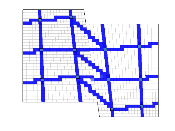
Visualize the dual grid¶

We plot the edges between the coarse block centroids

clf;
plotDual(G, DG)
view(0,0); axis tight off;

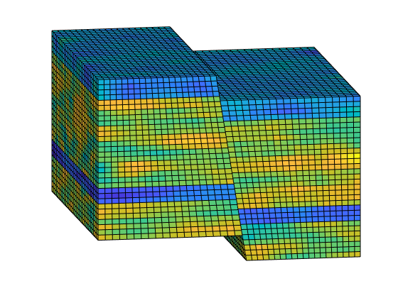
Define permeability and fluid¶

Disable gravity. Can be enabled if one finds that sort of thing interesting.

gravity off;
% Instansiate a fluid object for one phase flow.
fluid        = initSingleFluid('mu' ,    1*centi*poise     , ...
                               'rho', 1014*kilogram/meter^3);
% Create layered permeability in logical indices to emulate sedimentary
% rocks across the fault
layers       = [100 400 50 350];
K            = logNormLayers([nx, ny, nz], layers);
rock.perm    = convertFrom(K(1:G.cells.num), milli*darcy);  % mD -> m^2
% Plot the permeability

clf;
plotCellData(G, log10(rock.perm));
view(-10,15); axis tight off;
T = computeTrans(G, rock);

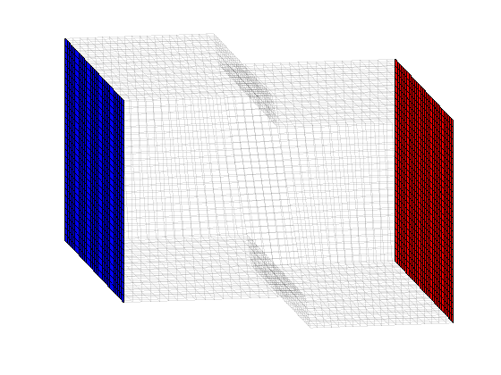
Add a simple Dirichlet pressure boundary¶

We add boundary conditions along the extremal values of the x axis.

bc = [];
% Find the edges and add unit and zero pressure boundary condition there
d  = abs(G.faces.centroids(:,1) - max(G.faces.centroids(:,1)));
ind1 = find (d < 1e6*eps);
bc = addBC(bc, ind1, 'pressure', 1);

d  = abs(G.faces.centroids(:,1) - min(G.faces.centroids(:,1)));
ind0 = find (d < 1e6*eps);
bc = addBC(bc, ind0, 'pressure', 0);

% Plot the faces selected for boundary conditions, with the largest
% pressure in red and the smallest in red.
clf;
plotGrid(G, 'FaceAlpha', 0, 'EdgeAlpha', .1);
plotFaces(G, ind1, 'FaceColor', 'Red')
plotFaces(G, ind0, 'FaceColor', 'Blue')
view(-10,15); axis tight off;

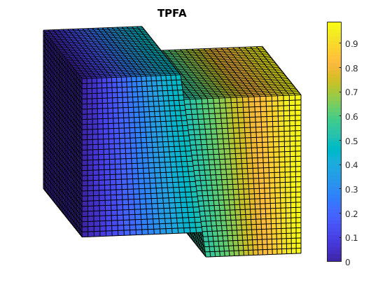
Solve the pressure system¶

First we initiate a pressure system. This structure is always required, but without transport only the grid is relevant.

sol = initState(G, [], 0, 1);

% Solve TPFA reference solution.
solRef = incompTPFA(sol, G, T, fluid, 'bc', bc);

% Solve multiscale pressure. Reconstruct conservative flow using flow basis
% functions.
solMSFV = solveMSFV_TPFA_Incomp(sol, G, CG, T, fluid, 'Dual', DG, ...
    'Reconstruct', true, 'bc', bc, 'Verbose', false, 'SpeedUp', true);

Warning: solveMSFV_TPFA_Incomp is DEPRECATED! Please use incompMultiscale from
the "msrsb" module instead.

Plot TPFA solution¶

clf;
plotCellData(G, solRef.pressure);
view(-10,15); axis tight off; colorbar;
set(gca, 'CLim', [0, max(solRef.pressure)]);
title('TPFA')

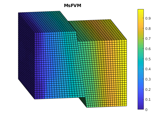
Plot MSFVM solution¶

clf;
plotCellData(G, solMSFV.pressure);
view(-10,15); axis tight off; colorbar;
title('MsFVM')
% Use same axis scaling as the TPFA solution
set(gca, 'CLim', [0, max(solRef.pressure)]);

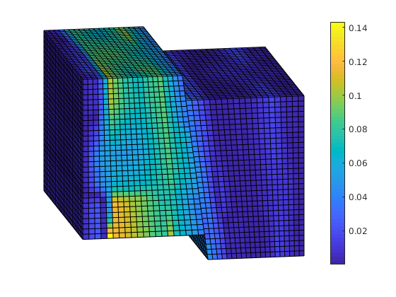
Plot error¶

reportError(solRef.pressure, solMSFV.pressure);
clf;
% Plot the error scaled with local variation
plotCellData(G, abs(solRef.pressure - solMSFV.pressure) ./ abs(max(solRef.pressure - min(solRef.pressure))));
view(-10,15); axis tight off; colorbar;

ERROR:
      2: 0.08070356
      Sup: 0.23359118
      Minimum 0.00000711

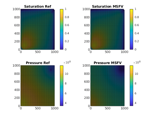
A simple two phase problem solved using the Multiscale Finite Volume method¶

Generated from simple2phMsFV.m

The multiscale finite volume method can easily be used in place of a regular pressure solver for incompressible transport. This example demonstrates a two phase solver on a 2D grid.

mrstModule add coarsegrid msfvm incomp msrsb

Construct simple 2D Cartesian test case¶

nx = 50; ny = 50;
Nx = 5; Ny = 5;
G         = cartGrid([nx, ny], [1000, 1000]);
G         = computeGeometry(G);

% Plot each timestep
doPlot = true;

p  = partitionUI(G, [Nx, Ny]);
CG = generateCoarseGrid(G, p);
CG = coarsenGeometry(CG);

Generate dual grid¶

DG = partitionUIdual(CG, [Nx, Ny]);
CG.dual = DG;

Visualize¶

clf;
plotDual(G, DG)

Uniform permeability¶

rock = makeRock(G, 100*milli*darcy, 0.3);
T = computeTrans(G, rock);

Define a simple 2 phase fluid¶

fluid = initSimpleFluid('mu' , [   1,  10]*centi*poise     , ...
                        'rho', [1014, 859]*kilogram/meter^3, ...
                        'n'  , [   2,   2]);

Setup a producer / injector pair of wells¶

rate = 0.01*meter^3/second;
bhp  = 100*barsa;
radius = 0.05;
% Injector in lower left corner
W = [];
W = verticalWell(W, G, rock, 5, 5, [],      ...
            'Type', 'rate' , 'Val', rate, ...
            'Radius', radius, 'InnerProduct', 'ip_tpf', ...
            'Comp_i', [1, 0]);
% Producer in upper right corner
W = verticalWell(W, G, rock, nx - 5, ny - 5, [],     ...
            'Type', 'bhp' , 'Val', bhp, ...
            'Radius', radius, 'InnerProduct', 'ip_tpf', ...
            'Comp_i', [0, 1]);

Set up solution structures with only one phase¶

refSol    = initState(G, W, 0, [0, 1]);
msSol     = initState(G, W, 0, [0, 1]);

gravity off
verbose = false;

Set up pressure and transport solvers¶

Reference TPFA

r_psolve = @(state) incompTPFA(state, G, T, fluid, 'wells', W);
% MsFV solver. We use the more modern version of the solver found in the
% msrsb module. From the linear system A, we construct a set of msfv basis
% functions.
A = getIncomp1PhMatrix(G, T, msSol, fluid);
basis = getMultiscaleBasis(CG, A, 'type', 'msfv');
psolve = @(state) incompMultiscale(state, CG, T, fluid, basis, 'Wells', W);
% Implicit transport solver
tsolve   = @(state, dT) implicitTransport(state, G, dT, rock, ...
                                                fluid, 'wells', W, ...
                                                'verbose', verbose);

Processing block 1 of 36...
Processing block 2 of 36...
Processing block 3 of 36...
Processing block 4 of 36...
Processing block 5 of 36...
Processing block 6 of 36...
Processing block 7 of 36...
Processing block 8 of 36...
...

Alternatively we could have defined an explicit transport solver by tsolve = @(state, dT, fluid) explicitTransport(state, G, dT, rock, fluid, … ‘wells’, W, ‘verbose’, verbose);

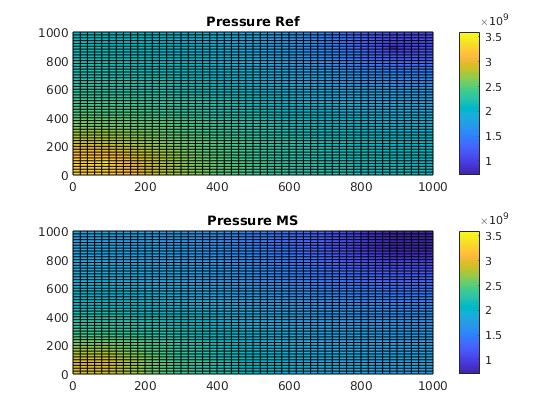
Solve initial pressure in reservoir¶

We solve and plot the pressure in the reservoir at t=0.

refSol= r_psolve(refSol);
msSol = psolve(msSol);
subplot(2,1,1)
plotCellData(G, refSol.pressure); axis tight; colorbar;
title('Pressure Ref')
cbar = caxis();
subplot(2,1,2)
plotCellData(G, msSol.pressure); axis tight; colorbar;
title('Pressure MS')
caxis(cbar)

Transport loop¶

We solve the two-phase system using a sequential splitting in which the pressure and fluxes are computed by solving the flow equation and then held fixed as the saturation is advanced according to the transport equation.

time   = 1*year;
dT     = time/60;

Start the main loop¶

Iterate through the time steps and plot the saturation profiles along the way.

t = 0;
while t < time
    % Solve transport equations using the transport solver
    msSol  = tsolve(msSol , dT);
    refSol = tsolve(refSol, dT);

    % Update the pressure based on the new saturations
    msSol    = psolve(msSol);
    refSol   = r_psolve(refSol);
    % Increase time and continue if we do not want to plot saturations
    if doPlot
        clf;
        % Saturation plot
        subplot(2,2,1)
        plotGrid(G, 'FaceColor', 'None', 'EdgeAlpha', 0)
        plotCellData(G, refSol.s(:,1), refSol.s(:,1) > 1e-4); axis tight; colorbar;
        title('Saturation Ref')
        caxis([0 1]);
        subplot(2,2,2)
        plotGrid(G, 'FaceColor', 'None', 'EdgeAlpha', 0)
        plotCellData(G, msSol.s(:,1), msSol.s(:,1) > 1e-4); axis tight; colorbar;
        title('Saturation MSFV')
        % Align colorbars
        caxis([0 1])
        % Pressure plot
        subplot(2,2,3)
        plotCellData(G, refSol.pressure); axis tight; colorbar;
        title('Pressure Ref')
        minP = min(min(refSol.pressure), min(msSol.pressure));
        maxP = max(max(refSol.pressure), max(msSol.pressure));
        cbar = [minP, maxP];
        subplot(2,2,4)
        hs = plotCellData(G, msSol.pressure); axis tight; colorbar;
        title('Pressure MSFV')
        caxis(cbar)
        drawnow
    end
    t = t + dT;
end

Multiscale Finite Volume Pressure solver: Iterative improvements¶

Generated from simpleIterativeMSFVMExample.m

The Multiscale Finite Volume Method can be used in smoother-multiscale cycles or as a preconditioner for iterative algorithms. This example demonstrates this usage in preconditioned GMRES and Dirichlet Multiplicative / Additive Schwarz smoothing cycles.

Iteration parameters¶

We will be doing 100 iterations in total, corresponding to 100 GMRES iterations and 10 cycles of 10 smoothings for the MsFV iterations. Omega is initially set to 1.

omega = 1;
subiter = 10;
iterations = 100;
cycles = round(iterations/subiter);

Load required modules¶

mrstModule add coarsegrid msfvm incomp

Define a simple 2D Cartesian grid¶

We create a

fine grid, and a coarse grid of $5 times 5$ giving each coarse block

fine cells. We also add geometry data to the grids.

nx = 50; ny = 50;
Nx = 5; Ny = 5;
% Instansiate the actual grid
G = cartGrid([nx, ny]);
G = computeGeometry(G);
% Generate coarse grid
p = partitionUI(G, [Nx, Ny]);
CG = generateCoarseGrid(G, p);
CG = coarsenGeometry(CG);

Dual grid¶

Generate the dual grid logically and plot it.

DG = partitionUIdual(CG, [Nx, Ny]);
% Plot the dual grid
clf;
plotDual(G, DG)
view(0,90), axis tight

_images/simpleIterativeMSFVMExample_01.png

Permeability and fluid¶

We define a single phase fluid.

fluid        = initSingleFluid('mu' ,    1*centi*poise     , ...
                                'rho', 1014*kilogram/meter^3);
% Generate a lognormal field via porosity
poro = gaussianField(G.cartDims, [.2 .4], [11 3 3], 2.5);
K = poro.^3.*(1e-5)^2./(0.81*72*(1-poro).^2);
rock.perm    = K(:);
clf;
plotCellData(G, log10(rock.perm));
axis tight off;

_images/simpleIterativeMSFVMExample_02.png

Add a simple Dirichlet boundary¶

bc = [];
bc = pside   (bc, G, 'LEFT', .5*barsa());
bc = pside   (bc, G, 'RIGHT', .25*barsa());

Add some wells near the corners¶

W = [];
cell1 = round(nx*1/8) + nx*round(ny*1/8);
cell2 = round(nx*7/8) + nx*round(ny*7/8);

W = addWell(W, G, rock, cell1,      ...
            'Type', 'bhp' , 'Val', 1*barsa(), ...
            'Radius', 0.1, 'InnerProduct', 'ip_tpf', ...
            'Comp_i', 0);

W = addWell(W, G, rock, cell2,      ...
            'Type', 'bhp' , 'Val', 0*barsa(), ...
            'Radius', 0.1, 'InnerProduct', 'ip_tpf', ...
            'Comp_i', 0);

State and tramsmissibility¶

Instansiate empty well and calculate transmissibility.

sol = initState(G, [], 0, 1);
T = computeTrans(G, rock);

Solve the systems¶

We define an anonymous function because many parameters are common to each call tol solveMSFVM_TPFA_Incomp. This makes it easy to compare different parameters without duplicating code.

solvems = @(iterations, subiterations, iterator, smoother, omega) ...
        solveMSFV_TPFA_Incomp(sol, G, CG, T, fluid, 'Wells', W, ...
        'Dual', DG, 'bc', bc,...
        'Iterations',       iterations,...
        'Subiterations',    subiterations,...
        'Iterator',         iterator,...
        'Smoother',         smoother,...
        'Omega',            omega, ...
        'Verbose',          false);

disp 'Solving reference solution';
tic; solRef = incompTPFA(sol, G, T, fluid, 'bc', bc, 'wells', W); toc;
disp 'Solving without iterations';
tic; solFV_noiter = solvems(0, 0, '', '', 0); toc;
disp 'Solving with GMRES using MsFV preconditioner';
tic; solFV_gmres = solvems(iterations, 0, 'gmres', '', 0) ;toc;
disp 'Solving with GMRES without preconditioner';
tic; solFV_direct =solvems(iterations, 0, 'gmres-direct', '', 0) ;toc;
disp 'Solving with Dirichlet Multiplicative Schwarz (DMS) smoother cycles';
tic; solFV_dms = solvems(cycles, subiter, 'msfvm', 'DMS', omega);toc;
disp 'Solving with Dirichlet Additive Schwarz (DAS) smoother cycles';
tic; solFV_das = solvems(cycles, subiter, 'msfvm', 'DAS', omega);toc;

Solving reference solution
Elapsed time is 0.020714 seconds.
Solving without iterations
Warning: solveMSFV_TPFA_Incomp is DEPRECATED! Please use incompMultiscale from
the "msrsb" module instead.
Elapsed time is 0.030138 seconds.
Solving with GMRES using MsFV preconditioner
Warning: solveMSFV_TPFA_Incomp is DEPRECATED! Please use incompMultiscale from
...

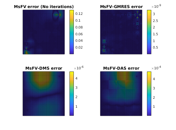
Plot error for the different configurations¶

clf;
subplot(2,2,1)
% We plot the error scaled with total variation in the reference solution.
variation = abs(max(solRef.pressure - min(solRef.pressure)));

plotCellData(G, abs(solRef.pressure - solFV_noiter.pressure) ./ variation);
view(0,90); axis tight off; colorbar;
title('MsFV error (No iterations)')
subplot(2,2,2)


plotCellData(G, abs(solRef.pressure - solFV_gmres.pressure) ./ variation);
view(0,90); axis tight off; colorbar;
title('MsFV-GMRES error')

subplot(2,2,3)
% Plot error scaled with local variation
plotCellData(G, abs(solRef.pressure - solFV_dms.pressure) ./ variation);
view(0,90); axis tight off; colorbar;
title('MsFV-DMS error')

subplot(2,2,4)
% Plot error scaled with local variation
plotCellData(G, abs(solRef.pressure - solFV_das.pressure) ./ variation);
view(0,90); axis tight off; colorbar;
title('MsFV-DAS error')

_images/simpleIterativeMSFVMExample_03.png

Plot smoother cycles¶

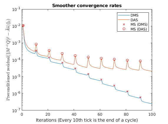
We plot the preconditioned residuals for the smoother cycles. Note that the residual decreases monotonically within a smoother cycle, but jumps back up when a MsFV solution is comptuted. This is because the new multiscale solution is recomptued with source terms to get a better approximation than the last smoother cycle. The end of a cycle is marked in red.

clf;

semilogy([solFV_dms.residuals; solFV_das.residuals]');
hold on
title('Smoother convergence rates');

xlabel(sprintf('Iterations (Every %dth tick is the end of a cycle)', subiter));
ylabel('Preconditioned residual($\|M^{-1}Q(\tilde{r} - \tilde{A}\tilde{u}) \|_2$)','interpreter','latex')
t_ms = 1:subiter:iterations;

semilogy(t_ms, solFV_dms.residuals(t_ms), 'rx')
semilogy(t_ms, solFV_das.residuals(t_ms), 'ro')
legend({'DMS','DAS', 'MS (DMS)', 'MS (DAS)'});

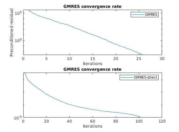
_images/simpleIterativeMSFVMExample_04.png

Plot residuals for GMRES¶

The residuals of the preconditioned GMRES are not directly comparable to GMRES without preconditioner, but we can compare the number of iterations.

clf;subplot(2,1,1)
semilogy([solFV_gmres.residuals]');
title('GMRES convergence rate'); legend({'GMRES'});
xlabel('Iterations');
ylabel('Preconditioned residual')

subplot(2,1,2);
semilogy([solFV_direct.residuals]');
title('GMRES convergence rate'); legend({'GMRES-direct'});
xlabel('Iterations');

_images/simpleIterativeMSFVMExample_05.png

Check error¶

Note that while the norms are different, the preconditioned GMRES converges while the direct GMRES does not. They both start with the same initial pressure solution. To see that the preconditioner ends up with a better result, we can compare the final pressure solutions:

disp 'With preconditioner:'
reportError(solRef.pressure, solFV_gmres.pressure);
disp 'Without preconditioner:'
reportError(solRef.pressure, solFV_direct.pressure);

With preconditioner:
ERROR:
      2: 0.00000000
      Sup: 0.00000000
      Minimum 0.00000000
Without preconditioner:
ERROR:
      2: 0.00102428
...

Multiscale Finite Volume Pressure Solver¶

Generated from simpleMSFVExample.m

This example compares the multiscale finite volume method with a fine scale solution for a simple case of single phase incompressible flow with wells and boundary conditions on a Cartesian grid. The Multiscale Finite Volume Method (MsFVM) is a multiscale method where instead of solving a full discretization for all fine cells, a series of smaller, local problems are solved with unit pressure to give a coarse pressure system. The resulting coarse pressure is then used to scale the local problems to find a fine scale pressure approximation. The method is attractive because pressure updates are inexpensive once the pressure basis functions have been constructed and because it guarantees a conservative flow field if an additional set of basis functions are created.

Load the modules required for the example¶

We will use streamlines and coarse grids.

mrstModule add coarsegrid streamlines msfvm incomp

We define a simple 2D Cartesian grid¶

The fine scale grid will consist of

fine cells, with a coarse grid of

coarse blocks.

nx = 50; ny = 50;

Nx = 3; Ny = 3;

% Instansiate the fine grid
G = cartGrid([nx, ny]);
G = computeGeometry(G);

% Generate coarse grid
p = partitionUI(G, [Nx, Ny]);
CG = generateCoarseGrid(G, p);
CG = coarsenGeometry(CG);

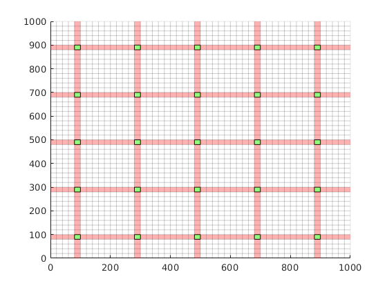
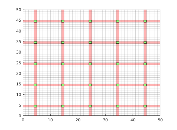
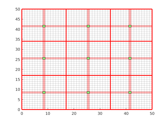
Generate dual grid from the coarse grid using a logical algorithm¶

The dual grid is based on the coarse grid and has corners defined by the coarse centroids of the coarse grid. Here our grid is Cartesian which makes it easy to define a dual grid based on the logical indices. We also visualize the dual grid. Cells corresponding to primal coarse centers are drawn in green, edge cells are drawn in orange and the primal coarse grid is drawn in red. Note that while the coarse grid is face centered, the dual coarse grid is cell centered, giving overlap between edges.

DG = partitionUIdual(CG, [Nx, Ny]);


clf;
plotDual(G, DG)
outlineCoarseGrid(G,p, 'red')
view(0,90), axis tight

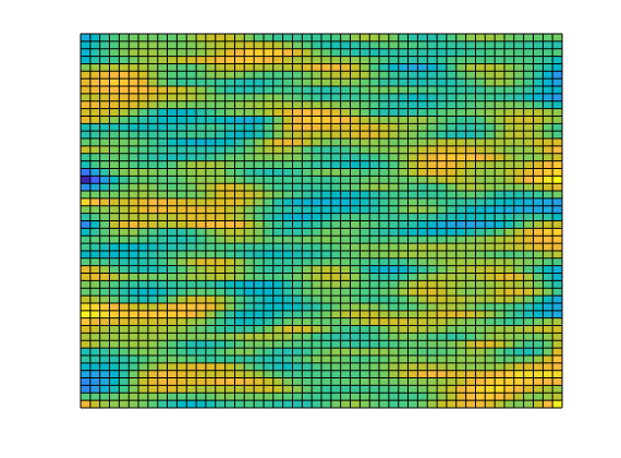
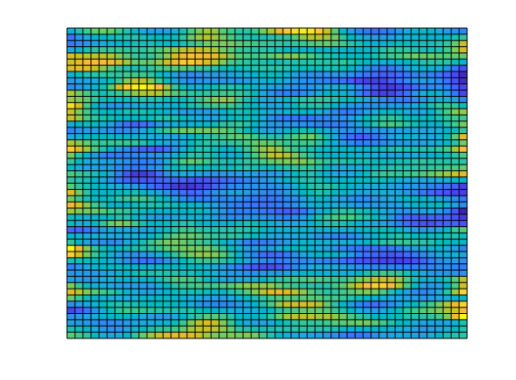
Set up permeability and fluid¶

We create a fluid object for one phase flow. The permeability is generated via a porosity distribution, which is then visualized.

fluid        = initSingleFluid('mu' ,    1*centi*poise     , ...
                                'rho', 1014*kilogram/meter^3);
% Permeability
poro = gaussianField(G.cartDims, [.4 .8], [11 3 3], 2.5);
K = poro.^3.*(1e-5)^2./(0.81*72*(1-poro).^2);
rock.perm    = K(:);

% Plot log10 of permeability
clf;
plotCellData(G, log10(rock.perm));
axis tight off;

Add a simple Dirichlet boundary¶

Add a simple flow boundary condition based on pressure. This gives flow everywhere.

bc = [];
bc = pside   (bc, G, 'LEFT' , 1*barsa());
bc = pside   (bc, G, 'RIGHT', 0);

Add wells¶

We are adding a producer / injector pair of wells to demonstrate their effect on the solver.

W = [];
cell1 = 13 + ny*13;
cell2 = 37 + ny*37;


W = addWell(W, G, rock, cell1,      ...
            'Type', 'bhp' , 'Val', .0*barsa(), ...
            'Radius', 0.1, 'InnerProduct', 'ip_tpf', ...
            'Comp_i', 0);

W = addWell(W, G, rock, cell2,      ...
            'Type', 'bhp' , 'Val', 1*barsa(), ...
            'Radius', 0.1, 'InnerProduct', 'ip_tpf', ...
            'Comp_i', 0);

Solve the systems.¶

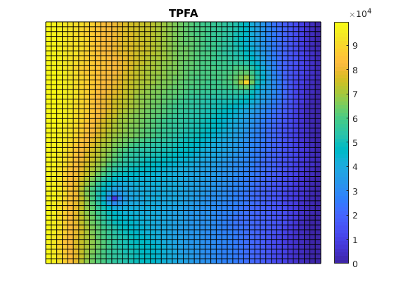
First we initiate a pressure system. This structure is always required, but without transport only the grid is relevant. We also compute transmissibilities. The MS solver is based on the TPFA solver, and as such has many of the same arguments. Multiscale methods in general can be seen as approximations to a specific discretization, and will inherit any strengths and weaknesses from the parent method, for instance grid orientation effects. The system is then solved three times: Once with a full TPFA solver, once with the multiscale sovler with conservative flow and lastly using the multiscale solver without conservative flow.

sol = initState(G, [], 0, 1);

T = computeTrans(G, rock);

% Solve TPFA reference solution.
solRef = incompTPFA(sol, G, T, fluid, 'wells', W, 'bc', bc);

% Solve multiscale pressure. Reconstruct conservative flow using flow basis
% functions.
solMSFV = solveMSFV_TPFA_Incomp(sol, G, CG, T, fluid,...
                                'Wells', W,...
                                'bc', bc,...
                                'Dual', DG,...
                                'Reconstruct', true,...
                                'Verbose', false);

solMSFV2 = solveMSFV_TPFA_Incomp(sol, G, CG, T, fluid,...
                                'Wells', W,...
                                'bc', bc,...
                                'Dual', DG,...
                                'Reconstruct', false,...
                                'Verbose', false);

Warning: solveMSFV_TPFA_Incomp is DEPRECATED! Please use incompMultiscale from
the "msrsb" module instead.
Warning: solveMSFV_TPFA_Incomp is DEPRECATED! Please use incompMultiscale from
the "msrsb" module instead.

Plot reference solution¶

clf;
plotCellData(G, solRef.pressure);
axis tight off; colorbar;
set(gca, 'CLim', [0, max(solRef.pressure)]);
title('TPFA')

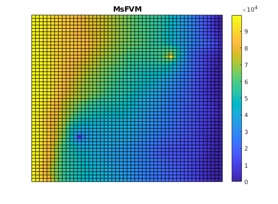
Plot the multiscale solution¶

clf;
plotCellData(G, solMSFV.pressure);
axis tight off; colorbar;
title('MsFVM')
% Use same axis scaling for the multiscale solution as the TPFA solution
set(gca, 'CLim', [0, max(solRef.pressure)]);

Plot error¶

Plot error scaled with local variation

reportError(solRef.pressure, solMSFV.pressure);
clf;
plotCellData(G, abs(solRef.pressure - solMSFV.pressure) ./ ...
                abs(max(solRef.pressure - min(solRef.pressure))));
axis tight off; colorbar;

ERROR:
      2: 0.04255786
      Sup: 0.10832201
      Minimum 0.00155851

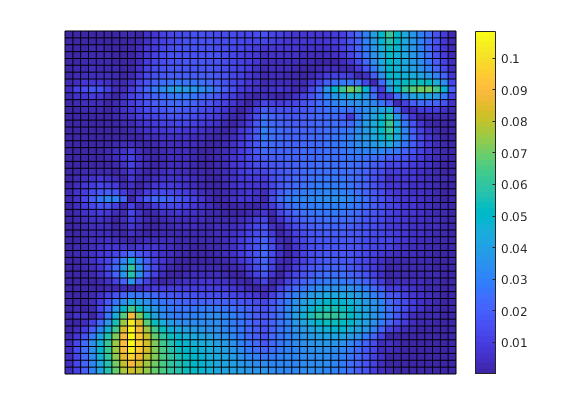
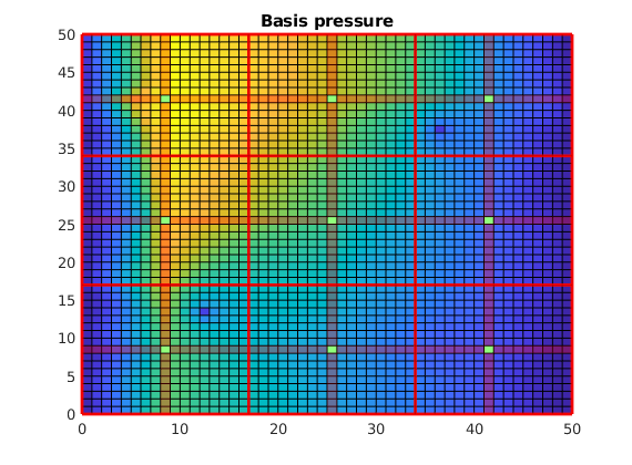
Decompose the solution¶

We observe that the error is large near the wells. This is not a coincidence: The MsFV solves bases its initial pressure solution of a coarse system, which does not actually include wells other than in a integral sense. We can decompose the solution to see this:

% Find the pressure basis
p_basis = solMSFV.msfvm.B*solMSFV.pressurecoarse;
p_corr = solMSFV.msfvm.Cr;
P = solMSFV.P';
% We need to permute this back to the original grid ordering using the
% permutation matrix...
p_basis = P*p_basis;
p_corr  = P*p_corr;

Plot the basis solution¶

Note that the pressure has become low where the wells are! This happens because the system simultanously tries to create correct flux over the edges of the coarse grid as if the wells were there, but tries to find a pressure solution where the wells are not actually included. This leads to low pressure. However, a set of correction functions are constructed, which add inn fine scale behavior of the wells as well as boundary conditions:

clf;
plotCellData(G, p_basis)
title('Basis pressure');
outlineCoarseGrid(G,p, 'red')
plotDual(G, DG)

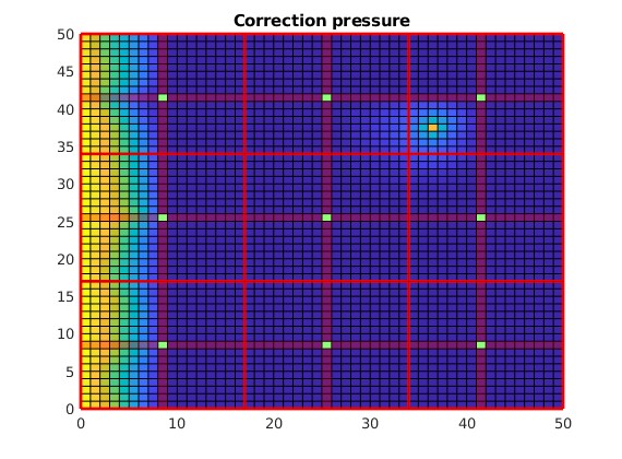
Plot the correction functions¶

The actual pressure is the sum of these two solutions. Note that when applied as an iterative method, the correction functions also contain non-local effects, i.e. source terms trying to minimze the residual.

clf;
plotCellData(G, p_corr)
title('Correction pressure')
outlineCoarseGrid(G,p, 'red')
plotDual(G, DG)

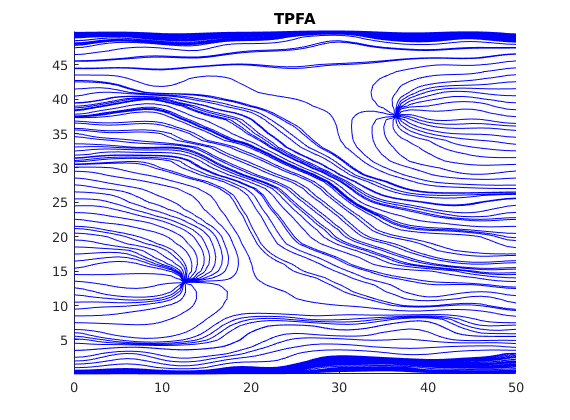
Plot streamlines for the reference¶

[i j] = ind2sub(G.cartDims, 1:G.cells.num);
% Start a streamline at all the boundaries, as well as in each well.
startpts = find(i == max(i) | i == min(i) | j == min(j) | j == max(j));
startpts = [startpts'; vertcat(W.cells)];

% Once a flux is plotted, reverse the flux to get more streamlines.
clf;
streamline(pollock(G, solRef, startpts));
tmp.flux = -solRef.flux;
streamline(pollock(G, tmp, startpts));
title('TPFA')
axis tight

Plot streamlines for the multiscale solution¶

clf;
streamline(pollock(G, solMSFV, startpts));
tmp.flux = -solMSFV.flux;
streamline(pollock(G, tmp, startpts));
title('MsFVM')
axis tight

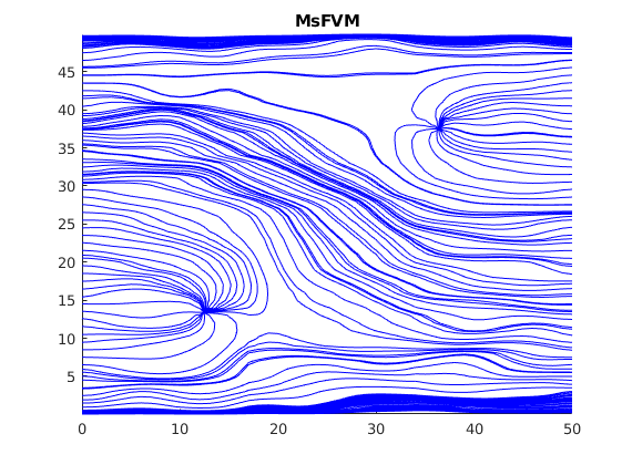
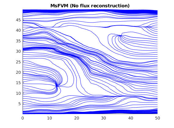
Plot streamlines without the reconstructed flux¶

Note that the reconstructed flux is much closer to the reference.

clf;
streamline(pollock(G, solMSFV2, startpts));
tmp.flux = -solMSFV2.flux;
streamline(pollock(G, tmp, startpts));
title('MsFVM (No flux reconstruction)')
axis tight

msfvm: Multiscale Finite-Volume method for pressure¶

Utilities¶

Examples¶

MsFV example on PEBI grid¶

Plot the coarse grids (dual and primal)¶

Set up boundary conditions and fluid¶

Set up the permeability¶

Solve the reference solution¶

Set up msfv solver and solve¶

Plot all solutions in seperate plots and the error¶

Example demonstrating the effects of aspect ratios and contrast on msfvm¶

Define a wide range of numerical experiments¶

Plot the numerical results¶

Plot the pressures¶

Example demonstrating Multiscale Finite Volume Solver over a fault for a corner point grid.¶

Load the modules required for the example¶

Define grid¶

Generate the coarse grid¶

Load the corresponding dual grid¶

Visualize the dual grid¶

Define permeability and fluid¶

Add a simple Dirichlet pressure boundary¶

Solve the pressure system¶

Plot TPFA solution¶

Plot MSFVM solution¶

Plot error¶

A simple two phase problem solved using the Multiscale Finite Volume method¶

Construct simple 2D Cartesian test case¶

Generate dual grid¶

Visualize¶

Uniform permeability¶

Define a simple 2 phase fluid¶

Setup a producer / injector pair of wells¶

Set up solution structures with only one phase¶

Set up pressure and transport solvers¶

Solve initial pressure in reservoir¶

Transport loop¶

Start the main loop¶

Multiscale Finite Volume Pressure solver: Iterative improvements¶

Iteration parameters¶

Load required modules¶

Define a simple 2D Cartesian grid¶

Dual grid¶

Permeability and fluid¶

Add a simple Dirichlet boundary¶

Add some wells near the corners¶

State and tramsmissibility¶

Solve the systems¶

Plot error for the different configurations¶

Plot smoother cycles¶

Plot residuals for GMRES¶

Check error¶

Multiscale Finite Volume Pressure Solver¶

Load the modules required for the example¶

We define a simple 2D Cartesian grid¶

Generate dual grid from the coarse grid using a logical algorithm¶

Set up permeability and fluid¶

Add a simple Dirichlet boundary¶

Add wells¶

Solve the systems.¶

Plot reference solution¶

Plot the multiscale solution¶

Plot error¶

Decompose the solution¶

Plot the basis solution¶

Plot the correction functions¶

Plot streamlines for the reference¶

Plot streamlines for the multiscale solution¶

Plot streamlines without the reconstructed flux¶

`msfvm`: Multiscale Finite-Volume method for pressure¶