`diagnostics`: Flow diagnostics functionality¶

Flow diagnostics refers to a set of simple and controlled numerical flow experiments that are run to probe a reservoir model, establish connections and basic volume estimates, compute dynamic heterogeneity measures, and and quickly provide a qualitative picture of the flow patterns in the reservoir. Flow diagnostics can also be used to compute simplified forecasts of fluid displacement and perform what-if and sensitivity analyzes in parameter regions surrounding preexisting simulations. The module offers a computationally inexpensive alternative to performing full-featured multiphase simulations to rank, compare, and validate reservoir models, upscaling procedures, and optimize production scenarios.

Contents¶: Files computeFandPhi - Compute flow-capacity/storage-capacity diagram (F,Phi) computeFandPhiFromDist - Undocumented Utility Function computeLorenz - Compute the Lorenz coefficient computeRTD - Compute residence time distributions based on computed tof-values computeSweep - Compute sweep efficiency versus dimensionless time (PVI) computeTOFandTracer - Compute time-of-flight and tracer distribution using finite-volume scheme. computeTOFandTracerAverage - Executes computeTOFandTracer for a series of states and averages computeTimeOfFlight - Compute time of flight using finite-volume scheme. computeWellPairs - Compute volumes and fluxes associated with each flux pair estimateRTD - Estimate residence time distributions based on computed tof-values expandCoarseWellCompletions - Pseudo-wells for computing flow diagnostics in an upscaled model expandWellCompletions - Pseudo-wells for computation of flow diagnostics for completions interactiveDiagnostics - Launch an interactive diagnostics session plotTOFArrival - Undocumented Utility Function plotTracerBlend - Visualise tracer partitions: gray regions are affected by multiple tracers plotWellAllocationComparison - Plot a panel comparing well-allocation from models with different resolution plotWellAllocationPanel - Plot a panel comparing well-allocation from models with different resolution plotWellPairConnections - Plot lines between wells to show relative flux allocation PostProcessDiagnostics - PostProcessDiagnostics handle class PostProcessDiagnosticsECLIPSE - Launch flow diagnostics postprocessor GUI for ECLIPSE simulation output. PostProcessDiagnosticsMRST - Launch flow diagnostics postprocessor GUI for MRST simulation output. selectTOFRegion - Select a subset of cells based on TOF criteria validateStateForDiagnostics - Validate and fix state for flow diagnostics

class PostProcessDiagnostics(dinput, precomp, varargin)¶

PostProcessDiagnostics handle class

Synopsis:

d = PostProcessDiagnostics(dinput, precomp, varargin)

Description:

Class definition for PostProcessDiagnostics GUI object. Takes a information from a previously run simulation and displays accompanying flow diagnostics and simulation results in an interactive GUI. If no precomputed diagnostics are passed in, diagnostics are calculated internally. Simulations should be processed first using either PostProcessDiagnosticsECLIPSE or PostProcessDiagnosticsMRST.

Keyword Arguments:
Parameters:	dinput – Structure containing the following fields: maxTOF - Maximum TOF value. G - MRST Grid structure with G.cells.PORV field Gs - Simulation Grid (for MRST simulations Gs = G) Data - Data structure containing static, dynamic and computed properties. precomp – Structure optionally containing array of precomputed diagnostics data for each timestep required. If empty, diagnostics will be calculated when the GUI is run.
	style – Optional gui style. Only default has been implemented.
Returns:	d – Handle to PostProcessDiagnostics object.

PostProcessDiagnosticsECLIPSE(varargin)¶

Launch flow diagnostics postprocessor GUI for ECLIPSE simulation output.

Synopsis:

[d] = PostProcessDiagnosticsECLIPSE(varargin)

Description:

Takes the output of an ECLIPSE simulation and launches the flow diagnostics postprocessor GUI. Optionally the path to the .EGRID file can be passed as an input parameter. If no parameters are given a file dialogue box will be launched to select the .EGRID file.

Keyword Arguments:
	steps – Array of timesteps to be displayed in the GUI. maxTOF – Maximum TOF value. Default value is 500 years. cleanup – true or false. Delete all existing flow diagnostics results from previous runs. Default is false. precompute – true or false. Precompute flow diagnostics for all timesteps. Default is true.
Returns:	d – Handle to PostProcessDiagnostics object.

See also

PostProcessDiagnosticsMRST.

PostProcessDiagnosticsMRST(problem, varargin)¶

Launch flow diagnostics postprocessor GUI for MRST simulation output.

Synopsis:

[d] = PostProcessDiagnosticsMRST(problem,varargin)

Description:

Takes the output of an MRST simulation problem and launches the flow diagnostics postprocessor GUI. The simulation should already have been run as PostProcessDiagnosticsMRST.m will only look for exisiting output.

Keyword Arguments:
Parameters:	problem – An MRST simulation problem defined using packSimulationProblem.m.
	steps – Array of timesteps to be displayed in the GUI. maxTOF – Maximum TOF value. Default value is 500 years. cleanup – true or false. Delete all existing flow diagnostics results from previous runs. Default is false. precompute – true or false. Precompute flow diagnostics for all timesteps. Default is true. startdate – optionally specify a start date of the format [day month year] e.g. [1 1 2000] for the 1st January 2000.
Returns:	d – Handle to PostProcessDiagnostics object.

See also

PostProcessDiagnosticsECLIPSE.

computeFandPhi(arg1, varargin)¶

Compute flow-capacity/storage-capacity diagram (F,Phi)

Synopsis:

[F,Phi] = computeFandPhi(pv, tof)
[F,Phi] = computeFandPhi(rtd)
[F,Phi] = computeFandPhi(rtd, 'sum', true/false);

Description:

Compute the flow-capacity/storage-capacity based upon either:

Pore volumes and time-of-flight values per cell. In this case, Phi is defined as the cumulative pore volume and F is the cumulative flux as function of residence time. Assuming incompressible flow, the instant flux is computed as the ratio of pore volume and the residence time.
Residence-time distribution. In this case, F is the integral of the RTD values, whereas Phi is the first-order moment (i.e., the integral of the product of time and RTD values).

Making an analogue to 1D displacement theory, the F-Phi curve is the equivalent to a plot of the fractional flow versus saturation. Technical description: see Section 13.2-13.3 in the MRST book, Shavali et al. (SPE 146446), and Shook and Mitchell (SPE 124625)

Parameters:	vol – pore volume, one value per cell tof – two-component vector with time-of-flight from injector and time-of-flight from producer, one value per cell rtd – structure with residence-time distribution from computeRTD
Returns:	F – flow capacity = cumulative flux for increasing time-of-flight values, where the flux per cell is defined from the relation volume = flux * total_travel_time Phi – storage capacity = cumulative pore volume for increasing time-of-flight values

computeFandPhiFromDist(RTD, varargin)¶: Undocumented Utility Function

computeLorenz(F, Phi)¶

Compute the Lorenz coefficient

Synopsis:

Lc = computeLorenz(F, Phi)

Parameters:	F – flow capacity Phi – storage capacity
Returns:	Lc – the Lorenz coefficient, a popular measure of heterogeneity. It is equal to twice the area under the curve and above the F=Phi line. It varies between 0 (homogeneous displacement) to 1 (infinitely heterogeneous displacement).

See also

computeFandPhi, computeSweep

computeRTD(state, G, pv, D, WP, W, varargin)¶

Compute residence time distributions based on computed tof-values .. rubric:: Synopsis:

dist = computeRTD(state, G, pv, D, WP, W, 'pn1', pv1, ...)

Description:

This function computes well-pair RTDs by simulating an imaginary tracer which ditributes equally among all phases (follows the total flux-field), and follows the flux field given by state. A tracer pulse is injected at injector i at time zero and produced at producer p. The RTD is scaled such that

RTD_{ip}(t) = (rate producer p / total tracer mass) * c_p(t),

where c_p(t) is the tracer concentration in producer p.

With the above scaling the RTD has units [s]^-1

the integral of the RTD approximates fractional recovery

(produced mass/injected mass)

the mean of the RTD time i-to-p allocation approximates the i-to-p allocation volume

RETURNS: dist - structure with fields

pairIx nreg x 2 each row index to injector/producer t nbin x 1 discrete times values nbin x 1 discrete RTD-values volumes nreg x 1 interaction volume for each well pair allocations nreg x 1 interaction allocation for each well pair injectorFlux ninj injector total rates producerFlux nprod producer total rates

SEE ALSO: estimateRTD

computeSweep(F, Phi)¶

Compute sweep efficiency versus dimensionless time (PVI)

Synopsis:

[Ev,tD] = computeSweep(F, Phi)

Parameters:	F – flow capacity Phi – storage capacity
Returns:	tD – dimensionless time (PVI) Ev – sweep efficiency. Analogue: 1D displacement using the F-Phi curve as flux funcion

See also

computeFandPhi, computeLorenz

computeTOFandTracer(state, G, rock, varargin)¶

Compute time-of-flight and tracer distribution using finite-volume scheme.

Synopsis:

D  = computeTOFandTracer(state, G, rock)
D  = computeTOFandTracer(state, G, rock, 'pn1', pv1, ...)

Description:

Construct the basis for flow diagnostic by computing

time-of-flight : nabla·(v T) = phi,
reverse time-of-flight: -nabla·(v T) = phi,
stationary tracer : ±nabla·(v C) = 0

using a first-order finite-volume method with upwind flux. A majority vote is also used to partition the volume and assign each cell to a unique tracer. Optionally, the routine can also compute time-of-flight values for each influence region by solving localized time-of-flight equations

nabla·(v C_i T) = phi C_i,

where C_i is the tracer concentration of each influence region.

Finally, first arrival time is computed by a graph algorithm.

Parameters:	G – Grid structure. rock – Rock data structure. Must contain a valid porosity field, ‘rock.poro’. state – Reservoir and well solution structure either properly initialized from functions ‘initResSol’ and ‘initWellSol’ respectively, or the results from a call to function ‘solveIncompFlow’. Must contain valid cell interface fluxes, ‘state.flux’.

OPTIONAL PARAMETERS (supplied in ‘key’/value pairs):

wells - Well structure as defined by function ‘addWell’. May be empty: (i.e., wells = []) which is interpreted as a model without any wells.
src - Explicit source contributions as defined by function: ‘addSource’. May be empty (i.e., src = []) which is interpreted as a reservoir model without explicit sources.
bc - Boundary condition structure as defined by function ‘addBC’.: This structure accounts for all external boundary conditions to the reservoir flow. May be empty (i.e., bc = []) which is interpreted as all external no-flow (homogeneous Neumann) conditions.
tracerWells - Logical index vector indicating subset of wells for which: tracer-fields will be computed. Empty matrix (default) is interpeted as all true, i.e., compute tracer fields for all wells.
computeWellTOFs - Boolean variable. If true, time-of-flight values are: computed individually for each influence region by solving
firstArrival - Boolean variable. If true, compute first-arrival time by: a graph algorithm.
solver - Function handle to solver for use in TOF/tracer equations.: Default (empty) is matlab mldivide (i.e., )
maxTOF - Maximal TOF thresholding to avoid singular/ill-conditioned: systems. Default (empty) is 50*PVI (pore-volumes-injected).
processCycles - Extend TOF thresholding to strongly connected: components in flux graph by considering Dulmage-Mendelsohn decomposition (dmperm). Recommended for highly cyclic flux fields. Only takes effect if ‘allowInf’ is set to false.

Returns:

D – struct that contains the basis for computing flow diagnostics: ‘inj’ - list of injection wells ‘prod’ - list of production wells ‘tof’ - time-of-flight and reverse time-of-flight returned

as an array where the first (G.cells.num x 2) elements contain forward/backward TOF for the whole field, and any other columns optinally contain TOF values for individual influence regions

‘itracer’ - steady-state tracer distribution for injectors ‘ipart’ - tracer partition for injectors ‘ifa’ - first-arrival time injectors ‘ptracer’ - steady-state tracer distribution for producers ‘ppart’ - tracer partition for producers ‘pfa’ - first-arrival time for producers

computeTOFandTracerAverage(state, G, rock, varargin)¶

Executes computeTOFandTracer for a series of states and averages

Synopsis:

D  = computeTOFandTracerAverage(state, G, rock, 'pn1', pv1, ...)

Description:

Computes time of flight for a series of time steps and avarages.

Parameters:

G – Grid structure.
rock – Rock data structure. Must contain a valid porosity field, ‘rock.poro’.
state – Reservoir and well solution structure either properly initialized from functions ‘initResSol’ and ‘initWellSol’ respectively, or the results from a call to function ‘solveIncompFlow’. Must contain valid cell interface fluxes, ‘state.flux’.

Keyword Arguments:

wells – Well structure as defined by function ‘addWell’. May be empty (i.e., wells = []) which is interpreted as a model without any wells.
dt – List of timesteps to use in averaging
max_tof – Threshold
min_tof – Threshold
Additional parameters will be passed on to ‘computeTOFandTracer’, which
computes the flow diagnostics. See this function for further documentation.

Returns:

D – struct that contains the basis for computing flow diagnostics: ‘inj’ - list of injection wells ‘prod’ - list of production wells ‘tof’ - time-of-flight and reverse time-of-flight returned

as an (G.cells.num x 2) vector

‘itracer’ - steady-state tracer distribution for injectors ‘ipart’ - tracer partition for injectors ‘ptracer’ - steady-state tracer distribution for producers ‘ppart’ - tracer partition for producers ‘isubset’ - flooding volumes which satisfy the min/max tof

thresholds (if set). Represents a kind of frequency.

‘psubset’ - drainage volumes which satisfy the min/max tof: thresholds (if set). Represents a kind of frequency.

EXAMPLE:

See also

computeTOFandTracer

computeTimeOfFlight(state, G, rock, varargin)¶

Compute time of flight using finite-volume scheme.

Synopsis:

 T        = computeTimeOfFlight(state, G, rock)
 T        = computeTimeOfFlight(state, G, rock, 'pn1', pv1, ...)

[T, A]    = computeTimeOfFlight(...)
[T, A, q] = computeTimeOfFlight(...)

Description:

Compute time-of-flight by solving

v·nabla T = phi

using a first-order finite-volume method with upwind flux. Here, ‘v’ is the Darcy velocity, ‘phi’ is the porosity, and T is time-of-flight. The time-of-flight T(x) is the time it takes an inert particles that is passively advected with the fluid to travel from the nearest inflow point to the point ‘x’ inside the reservoir. For the computation to make sense, inflow points must be specified in terms of inflow boundaries, source terms, wells, or combinations of these.

Parameters:	G – Grid structure. rock – Rock data structure. Must contain a valid porosity field, ‘rock.poro’. state – Reservoir state structure, must contain valid cell interface fluxes, ‘state.flux’. Typically, ‘state’ will contain the solution produced by a flow solver like ‘incompTPFA’.

OPTIONAL PARAMETERS (supplied in ‘key’/value pairs):

wells - Well structure as defined by function ‘addWell’. May be empty

(i.e., wells = []) which is interpreted as a model without any wells.

src - Explicit source contributions as defined by function

‘addSource’. May be empty (i.e., src = []) which is interpreted as a reservoir model without explicit sources.

bc - Boundary condition structure as defined by function ‘addBC’.

This structure accounts for all external boundary conditions to the reservoir flow. May be empty (i.e., bc = []) which is interpreted as all external no-flow (homogeneous Neumann) conditions.

reverse - Boolean variable. If true, the reverse time-of-flight will be

computed, i.e., the travel time from a cell inside the reservoir to the nearest outflow point (well, source, or outflow boundary). Default: FALSE, i.e, compute forward tof.

tracer - Cell-array of cell-index vectors for which to solve a

stationary tracer equation:

nabla·(v C) = 0, C(inflow,t)=1

One equation is solved for each vector with tracer injected in the cells with the given indices. Each vector adds one additional right-hand side to the original tof-system. Output given as additional columns in T.

computeWellTOFs - Boolean variable. If true, time-of-flight values are

computed individually for each influence region by solving equations of the form:

nabla·(v C_i T) = phi C_i, T(inflow)=0

where C_i denotes the tracer concentration associated with each individual influence region

firstArrival - Boolean variable. If true, also compute the first-arrival

time by a graph algorithm (requires MATLAB R2015b or newer)

computeWellPairs(state, G, rock, W, D)¶

Compute volumes and fluxes associated with each flux pair

Synopsis:

WP = computeWellPairs(state, G, rock, W, D)

Parameters:

state – Reservoir state
G – Grid structure.
rock – Rock data structure. Must contain a valid porosity field, ‘rock.poro’.
state – Reservoir and well solution structure either properly initialized from functions ‘initResSol’ and ‘initWellSol’ respectively, or the results from a call to function ‘solveIncompFlow’. Must contain valid cell interface fluxes, ‘state.flux’.
W – Well structure
D – Struct containing TOF and tracer See documentation of computeTOFandTracer

Returns:

WP – struct containing well-pair diagnostics ‘pairs’ - list of well pairs (as text strings using well names) ‘pairsIx’ - list of well pairs (indices in a N_pair x 2 list. Pair

number i has injector pairsIx(i, 1) and producer pairsIx(i, 2)

‘vols’ - pore volumes associated with each pair ‘inj’ - list of structs containing allocation factors for the

injectors

‘prod’ - list of structs containing allocation factors for the

producers
The structs that contain flux allocation information consist of the
following data objects –

‘alloc’ - nxm array, where n is the number of perforations in

this well and m is the number of wells or segments from the flow diagnostics computation that may potentially contribute to the flux allocation

‘ralloc’ - nx1 array containing the well flux that cannot be

attributed to one of the wells/segments accounted for in the flow diagnostics computatation

‘z’ - nx1 array giving the depth of the completions ‘name’ - string with the name of the well or segment

estimateRTD(pv, D, WP, varargin)¶

Estimate residence time distributions based on computed tof-values

Synopsis:

dist = estimateRTD(pv, D, WP, 'pn1', pv1, ...)

Description:

This function estmates well-pair RTDs based on computed TOFs and tracer fields. The RDT approximates an imaginary tracer which ditributes equally among all phases (follows the total flux-field). A tracer pulse is injected at injector i at time zero and produced at producer p. The RTD is scaled such that

RTD_{ip}(t) ~= (rate producer p / total tracer mass) * c_p(t),

where c_p(t) is the tracer concentration in producer p.

With the above scaling the RTD has units [s]^-1

the integral of the RTD approximates fractional recovery

(produced mass/injected mass)

the mean of the RTD time i-to-p allocation approximates the i-to-p allocation volume

Returns:	dist – structure with fields pairIx nreg x 2 each row index to injector/producer t nbin x 1 discrete times values nbin x 1 discrete RTD-values volumes nreg x 1 interaction volume for each well pair allocations nreg x 1 interaction allocation for each well pair injectorFlux ninj injector total rates producerFlux nprod producer total rates

SEE ALSO: computeRTD

expandCoarseWellCompletions(xc, WC, Wdf, p)¶

Pseudo-wells for computing flow diagnostics in an upscaled model

Synopsis:

[xn, Wn] = expandCoarseWellCompletions(xc, Wc, Wdf, p)

Parameters:

xc – Reservoir and well solution structure either properly initialized from functions ‘initResSol’ and ‘initWellSol’, respectively, or the results from a call to function ‘solveIncompFlow’. Must contain valid cell interface fluxes, ‘state.flux’.
Wc – Well structure as defined by function ‘addWell’.
Wdf – Expanded well structure used for flow diagnostics computation in the underlying fine-scale model, typically the result of a call to ‘expandWellCompletions’.
p – partition vector describing the coarse-scale partition (i.e., the mapping from the fine grid to the coarse grid)

Returns:

Wn – Well structure containing the pseudo wells
xn – Reservoir and solution structure corresponding

expandWellCompletions(state, W, expansion, split)¶

Pseudo-wells for computation of flow diagnostics for completions

Synopsis:

[xn, Wn] = expandWellCompletions(x, W, c)

Description:

The routines in the flow diagnostic module compute time-of-flight, tracer partition, and well-pair information associated with the whole completion set of each individual well. To compute flow diagnostics for subsets of the well completion, the corresponding well must be replaced by a set of pseudo wells, one for each desired completion interval.

Parameters:

x – Reservoir and well solution structure either properly initialized from functions ‘initResSol’ and ‘initWellSol’, respectively, or the results from a call to function ‘solveIncompFlow’. Must contain valid cell interface fluxes, ‘state.flux’.
W – Well structure as defined by function ‘addWell’.
expansion –
Either of two alternatives:
1. nx2 vector that specifies how to expand individual wells into a set of pseudo wells. That is, the completions of well number c(i,1) are assigned to c(i,2) bins using a load-balanced linear distribution and then the well is replaced with c(i,2) pseudo wells, one for each bin of completions.
2. Cell array of length n. Entry number i in this cell array should be the same length as W(i).cells and contain the bins that will be used to expand the well.

Returns:

Wn – Well structure containing the pseudo wells
xn – Reservoir and solution structure corresponding

interactiveDiagnostics(G, rock, W, varargin)¶

Launch an interactive diagnostics session

Synopsis:

interactiveDiagnostics(G, rock, W);
interactiveDiagnostics(G, rock, W, 'state', state)
interactiveDiagnostics(G, rock, W, dataset, 'state', state)

Description:

This function launches an interactive session for doing flow diagnostics. The functionality differs slightly based on the input arguments given:

If a dataset is given, this set of cellwise data will be available for visualization.

If a state is given, this state will allow for visualization of the component ratios inside a drainage volume. The flux from this state can also be used to calculate time of flight if “computeFlux” is disabled, for instance if the user has some external means of computing fluxes.

Once the initialization is complete, two windows will be produced:

A plotting window, showing the reservoir along with the wells and visualized quantities. In the plotting window, it is possible to click wells to get additional information, such as the allocation factors per perforation in the well, the phase distribution grouped by time of flight and the corresponding pore volumes swept/drained.
A controller window which is used to alter the state of the plotting window:

1) Wells can be selected for display (if a well is selected, the corresponding drainage (producer) or flooding (injector) volumes will be visualized. A simple playback function can be used to show propagation of time of flight. Different quantities can be visualized to get a better understanding of the system.

2) A set of buttons provide (experimental) well editing, access to visualization of the well pair connections, Phi/F diagram with Lorenz’ coefficient etc.

3) A player controller (experimental), if a time-series of wells (and states) are supplied.

Keyword Arguments:
Parameters:	G – Valid grid structure. rock – Rock with valid permeability and porosity fields. W – A set of wells which are compatible with the incompTPFA solver.
	‘state’ – Reservoir state containing fluid saturations and optionally flux and pressure (if ‘computeFlux’ is false) ‘computeGrid’ – Use G for plotting, but computeGrid for computing time-of-flight, tracer partitions, etc. ‘tracerfluid’ – Fluid used for tracer computation. This defaults to a trivial single-phase fluid. ‘fluid’ – Fluid used for mobility calculations if ‘useMobilityArrival’ is enabled. ‘LinSolve’ – Linear solver for pressure systems. Defaults: mldivide ‘computeFlux’ – If set to false, fluxes are extracted from the provided state keyword argument. This requires a state to be provided and can be used if the fluxes are computed externally (for instance from a expensive full-physics simulation) ‘useMobilityArrival’ – If the well plot showing nearby saturations should plot mobility instead of saturations. This may be interesting in some cases because the mobile fluids are more likely to be extracted. However, this plot is often dominated by very mobile gas regions. ‘daspect’ – Data aspect ratio, in a format understood by daspect() ‘name’ – Name to use for windows ‘leaveOpenOnClose’ – Default false. Leaves all figures open when closing the controller. ‘fastRotate’ – Enables fast rotate if true, disables if false. Default is enabled for models with > 50000 cells, disabled otherwise.
Returns:	Nothing. Creates two figures.

Example:

G = computeGeometry(cartGrid([10, 10, 2]));
rock = struct('poro', ones(G.cells.num, 1), 'perm', ones(G.cells.num, 1)*darcy)

W = verticalWell([], G, rock, 1,  1, [], 'Val', 1)
W = verticalWell(W, G, rock,  1,  10, [], 'Val', 1)
W = verticalWell(W, G, rock,  10, 1, [], 'Val', 1)
W = verticalWell(W, G, rock,  10, 10, [], 'Val', 1)
W = verticalWell(W, G, rock,  5,  5, [], 'Val', 0)
interactiveDiagnostics(G, rock, W);

See also

Diagnostics examples

plotTOFArrival(state, W, pv, fluid, prod, D, varargin)¶: Undocumented Utility Function

plotTracerBlend(G, partition, maxconc, varargin)¶

Visualise tracer partitions: gray regions are affected by multiple tracers

Synopsis:

 plotTracerBlend(G, partition, maxconc)
 plotTracerBlend(G, partition, maxconc, 'pn1', pv1, ...)

h = plotTracerBlend(...)

Parameters:

G – Grid structure partitioned by tracers.
partition – Tracer partition structure. This is the field ‘.ppart’ (or ‘.ipart’) of the diagnostics structure constructed by function ‘computeTOFandTracer’. One non-negative (integral) value for each grid cell.
maxconc – Maximum tracer concentration. One scalar value for each grid cell. This value is typically MAX(D.ptracer, [], 2).
'pn'/pv –
List of ‘key’/value pairs defining optional parameters. The supported options are:
- p – Power by which to amplify smearing effects. Note that the amplification power is applied to a decreasing function of concentration, so to highlight regions of smearing, small (but positive) powers should be used. Using p = 0.2 works well in the case of secondary production on the Tarbert layers of SPE10.
  Default value: p = 1. No special highlighting or amplification of smearing regions.
- alpha – Alpha factor to modify colormap for tracer. The colormap is by default set to be from the colorcube function. By specifying a value 0<alpha<=1, you can blend these colors with white to brigthen the colormap.
- cells – List of cells as expected by plotCellData()
- cmap – Colormap. Defaults to colorcube
non (Any) – matching parameter is passed through to plotCellData().

Returns:

h – Patch handle as defined by function ‘plotCellData’. Only returned if specifically requested.

Example:

[G, W, rock] = getSPE10setup(1:10);

is_pos = rock.poro > 0;
rock.poro(~is_pos) = min(rock.poro(is_pos));

T = computeTrans(G, rock);
fluid = initSingleFluid('mu' , 1*centi*poise, ...
                        'rho', 1000*kilogram/meter^3);
state = incompTPFA(initState(G, W, 0), G, T, fluid, 'wells', W);
D = computeTOFandTracer(state, G, rock, 'wells', W);

plotTracerBlend(G, D.ppart, max(D.ptracer, [], 2))

axis equal tight off, set(gca, 'DataAspectRatio', [ 1, 1, 0.1 ])

See also

computeTOFandTracer, plotCellData.

plotWellAllocationComparison(D1, WP1, D2, WP2, varargin)¶

Plot a panel comparing well-allocation from models with different resolution

SYNOPSIS: plotWellAllocationComparision(D1, WP1, D2, WP2)

Parameters:	D2 (D1,) – data structure with basic data for flow diagnostics computed by a call to ‘computeTOFandTracer’ for model 1 and model 2 WP2 (WP1,) – data structure containing information about well pairs, computed by a call to ‘computeWellPairs’

Description:

The routine makes a bar plot for each well segment that is represented in the input data D/WP. (There is no check that the well segments in D1 and D2 are the same). For injection wells, the bars represent the cumulative outfluxes, from the bottom to the top of the segment, that have been attributed to the different producers. The bars are shown in color for model 1, with a unique color representing each of the segments of the producers, and in solid black lines for model 2. For the production wells, the bars represent influxes that can be attributed to different injector segments. If the two models predict the same flux allocation, the color bars and the solid lines should be matching.

If D2 and WP2 are empty, a graph is produced that shows the well allocation for the wells in WP1.

See also

computeTOFandTracer, computeWellParis, expandWellCompletions

plotWellAllocationPanel(D, WP, varargin)¶

Plot a panel comparing well-allocation from models with different resolution

SYNOPSIS: plotWellAllocationPanel(D, WP)

Parameters:	D – data structure with basic data for flow diagnostics computed by a call to ‘computeTOFandTracer’ WP – data structure containing information about well pairs, computed by a call to ‘computeWellPairs’

Description:

The routine makes a bar plot for each well segment that is represented in the input data D/WP. For injection wells, the bars represent the cumulative outfluxes, from the bottom to the top of the segment, that have been attributed to the different producers. The bars are shown in color with a unique color representing each of the segments of the producers. For the production wells, the bars represent influxes that can be attributed to different injector segments.

plotWellPairConnections(G, WP, D, W, pv, minAlloc)¶

Plot lines between wells to show relative flux allocation

SYNOPSIS: plotWellPairConnections(G, WP, D, W, pv) plotWellPairConnections(G, WP, D, W, pv, mA)

Parameters:

G – Grid structure.
WP – data structure containing information about well pairs, computed by a call to ‘computeWellPairs’
D – data structure with basic data for flow diagnostics computed by a call to ‘computeTOFandTracer’
W – Well structure as defined by function ‘addWell’.
pv – vector with pore volume as computed by ‘poreVolume(G,rock)’
mA – disregard connections with relative allocation below mA

Description:

The routine makes a curved line between each well pair, where the thickness of the line is proportional to the relative flux allocation for this pair.

selectTOFRegion(D, max_tof, min_tof, varargin)¶

Select a subset of cells based on TOF criteria

Synopsis:

selectTOFRegion(D, max_tof, min_tof, ...);

Description:

Selects a subset of a grid based on TOF information and selection criteria.

Keyword Arguments:
Parameters:	D – Time of flight object computed by computeTOFandTracer. max_tof – All TOF-regions higher than this will be discarded. min_tof – All TOF-regions less than this will be discarded.
	‘drain_wells’ – List of draining (production) wells to consider. Other wells will be ignored ‘flood_wells’ – List of flooding (injecting) wells to consider. Other wells will be ignored ‘set_op’ – Operation op to perform, so that the computed selection is op(flood, drain) where flood and drain are the flooding and drainage volumes, respectively. ‘near_well_max_tof’ – Threshold for near well regions to include. Set to zero to disable including near-well regions. ‘psubset’ – User specified draining / production region to consider. When this is enabled, max_tof and min_tof will not be used to find the selected drainage region. ‘isubset’ – User specified flooding / injection region to consider. When this is enabled, max_tof and min_tof will not be used to find the selected flooding region. ‘tracer_threshold’ – Tracer-value threshold for including in region. For ‘intersection’, threshold applies to product of inj/prod tracers. Default value: 0.05;
Returns:	A list of cell indices

EXAMPLE:

See also

computeTOFandTracer.

Contents¶

OPTIMIZATION

Files: argmaxCubic - find max of cubic polynom through p1, p2 computeDefaultBasis - Undocumented Utility Function control2well - Update val-fields of W from controls u evalObjectiveDiagnostics - Undocumented Utility Function getObjectiveDiagnostics - Get an objective function for the diagnostics optimization routines lineSearch - lineSearch – helper function which performs line search based on linsolveWithTimings - Undocumented Utility Function optimizeDiagnosticsBFGS - Optimize well rates/bhps to minimize/maximize objective optimizeTOF - Optimize well rates based on diagnostics-based objective function optimizeWellPlacementDiagnostics - Optimize the placement of wells using flow diagnostics plotWellRates - Simple utility for plotting well rates. Used by optimizeTOF. plotWellsPrint - Plots wells as simple colored circles. Helper for diagnostics examples. solveStationaryPressure - Solve incompressible, stationary pressure without gravity with optional TOF output SolveTOFEqsADI - Solve the time of flight equations for solveStationaryPressure. tofRobustFix - Presently does nothing. Can be overriden if needed. unitBoxBFGS - Undocumented Utility Function well2control - Produce control vector u from target-wells

SolveTOFEqsADI(eqs, state, W, computeTracer, linsolve)¶

Solve the time of flight equations for solveStationaryPressure.

Synopsis:

D = SolveTOFEqsADI(eqs, state, W, true)

Description:

Solves tof/tracer problems efficiently for solveStationaryPressure. This function is primarily meant to be called from other functions and the interface reflects this. For a more general time of flight solver, see computeTOFandTracer.

Parameters:	eqs – Residual equations for pressure, time of flight and tracer. state – Reservoir state W – The wells for which tracers are to be computed. computeTracer – Boolean indicating if tracers are required.
Returns:	D – Time of flight / tracer structure.

argmaxCubic(p1, p2)¶: find max of cubic polynom through p1, p2

computeDefaultBasis(basis, G, state, system, W, fluid, pv, T, varargin)¶: Undocumented Utility Function

control2well(u, W, varargin)¶: Update val-fields of W from controls u If scaling is supplied, u is assumed to be scaled control s.t. 0<=u<=1 according to scaling.boxLims

evalObjectiveDiagnostics(u, obj, state, system, G, fluid, pv, T, W, scaling, varargin)¶: Undocumented Utility Function

getObjectiveDiagnostics(G, rock, type, varargin)¶

Get an objective function for the diagnostics optimization routines

Synopsis:

obj = getObjectiveDiagnostics(G, rock, 'minlorenz')

DESCRIPTION: This function produces a function handle that is a realization of some objective function based on quantities used in flow diagnostics, that is:

Pressure

Reservoir fluxes

Well fluxes and bottom hole pressure

Forward / backward time of flight

Well tracers (production / injection are treated seperately)

The returned function handle will accept input in the form

value = obj(state, D)

where state is the reservoir state and D the flow diagnostics object containing time of flight and tracer values. The ‘D’ struct can be returned from solveStationaryPressure or computeTOFandTracer and the state may come from any pressure solver contained in MRST. Most of the optimization routines get both these quantities from solveStationaryPressure, which is the recommended way of evaluating the objective functions if gradients are required.

The value return will be an instance of the ADI class and contains both the objective function value as well as gradients with respect to time of flight etc. The treatment is consistent with the ordering used in solveStationaryPressure.

Keyword Arguments:
Parameters:	G – The grid which will be used to evaluate the objective function rock – Rock with valid <poro> field containing the porosity. Several of the included objective functions use the pore volumes. type – Either: A string indicating the type of objective functions. Currently the available functions include, ‘minlorenz’ - Minimize the Lorenz’ coefficient, or A function handle which accepts a single struct argument containing the fields ’pressure’: Reservoir pressure ‘state’: Full reservoir state ‘pv’ : Pore volume ‘fluxes’: Well fluxes ‘bhp’: Well bottom hole pressures ‘forward_tof’: Time of flight originating from injectors ‘backward_tof’:Time of flight originating from producers This option is primarily intended for rapid experimentation, i.e. allowing someone who knows what they are doing to define objective functions on the fly in the form tmp = @(packed) sqrt(sum(packed.forward_tof.^2)) obj = getObjectiveDiagnostics(G, rock, tmp) which would make obj an objective function that is now the norm of the forward time of flight, and can be used to optimize well rates and placement.
	Any optional parameters are passed onto the objective function. Different objective functions handle different parameters.
Returns:	obj – Function handle accepting state and D struct.

lineSearch(u0, v0, g0, d, f, opt)¶

lineSearch – helper function which performs line search based on Wolfe-conditions.

SYNOPSIS: [u, v, g, info] = lineSearch(u0, v0, g0, d, f, opt)

PARAMETERS: u0 : current control vector v0 : current objective value g0 : current gradient d : search direction, returns an error unless d’*g0 > 0 f : objective function s.t. [v,g] = f(u) opt: struct of parameters for line search

RETURNS: u : control vector found along d v : objective value for u g : gradient for u info : struct containing fields:

flag : 1 for success (Wolfe conditions satisfied)

-1 max step-length reached without satisfying Wolfe-conds -2 line search failed in maxIt iterations (returns most recent control without further considerations)

step : step-length nits : number of iterations used

linsolveWithTimings(A, x, linsolve)¶: Undocumented Utility Function

optimizeDiagnosticsBFGS(G, W, fluid, pv, T, s, state, boxLims, objective, varargin)¶

Optimize well rates/bhps to minimize/maximize objective

Synopsis:

[W_best, D_init, D_best] = optimizeDiagnosticsBFGS(G, W, fluid, pv, T, s, state, minRate, objective)

Description:

Optimizes well rates/bhps as defined in W. The optimization process is based on BFGS where the search direction is projected onto the feasible domain as given by boxLims (upper/lower value for each control).

boxLims must be supplied for all target wells.

Keyword Arguments:
Parameters:	G – Valid grid structure. W – Well configuration suitable for AD-solvers. fluid – AD-fluid, for instance defined by initSimpleADIFluid. This is used to evalute relperm / viscosity when calculating fluxes. pv – Pore volume. Typicall output from poreVolume(G, rock). s – AD system. See initADISystem. state – Reservoir state as defined by initResSol. boxLims – Lower and upper limit for each target well objective – Objective function handle. Should have the interface @(state, D) where D is a diagnostics object (see computeTOFandTracer for the expected fields) and return a single numerical value along with its Jacobian. See getObjectiveDiagnostics for examples.
	maxiter – Maximum number of attempts to find an improvement. If maxiter successive evaluations fail to improve upon the last optimum, the function returns. alpha – Adjustment for scaling the initial relaxation factor in the optimization algorithm. This can improve convergence if the problem if chosen wisely, but the default is fairly robust since it is based on the magnitude of the initial objective as well as the gradients of the well at i = 0. targets – Index into W argument of wells that are to be optimized. They must all be initially the same type (i.e. producers / injectors) and they should be rate controlled. This defaults to all injectors with rate controls. deltatol – Termination criterion. If the relative change between iterations falls below this number, the function returns. For instance, if deltatol is 0.05, if the relative change between evaluations is less than 5% in absolute value, the iteration completes. plotProgress – Plots the well rates and function evaluations during the well optimization process. verbose – Controls the amount of output produced by the routine. linsolve – The linear solver used to solve the elliptic pressure systems during the optimization with a interface on the form @(A, b) for the linear system Ax=b. Fast multigrid or multiscale methods will significantly improve upon the solution speed for larger problems. alphamod – The modifier used to adjust alpha during the process. If a step is unsuccessful, alpha <- alpha/alphamod and the step is retried. If a step is successful, the next initial alpha is set to alpha <- alpha*alphamod.
Returns:	D_best – The flow diagnostics object corresponding to the best evaluated well configuration. W_best – The best well configuration history – A struct containing the optimization history in the fields: D - Diagnostic objects for all steps that reduced the objective function. values - Values per target well. One row per element in the D array. gradient - One gradient per diagnostics object. The objective function value for step i can be found at history.gradient(1).objective.val. iterations - Iteration per step required to improve upon the previous minimum.

optimizeTOF(G, W, fluid, pv, T, op, state, minRates, objective, varargin)¶

Optimize well rates based on diagnostics-based objective function

Synopsis:

[D_best, W_best, history] = optimizeTOF(G, W, fluid, pv, T, s, state, minRate, objective)
[D_best, W_best, history] = optimizeTOF(G, W, fluid, pv, T, s, state, minRate, objective, 'targets', [1, 3, 9])

Description:

Optimizes well rates. The optimization process is based on steepest descent given a gradient, and uses the following constraints to perform the optimization:

Sum of rates of the targets are constant, i.e. the total

injected/produced volume of the targets remains constant throughout the optimization.

All target wells must have a minimum rate which ensures that they do

not change from injectors to producers during the optimization process. This can be specified for all wells simultanously, or well specific limits can be provided.

The progress of the optimization can be visualized during the process (see optional parameters below)

Keyword Arguments:
Parameters:	G – Valid grid structure. W – Well configuration suitable for AD-solvers. fluid – AD-fluid, for instance defined by initSimpleADIFluid. This is used to evalute relperm / viscosity when calculating fluxes. pv – Pore volume. Typicall output from poreVolume(G, rock). op – Operators from setupOperatorsTPFA state – Reservoir state as defined by initResSol. minRates – Either a single value for the minimum well rate, or a value per target well (see ‘targets’ keyword) objective – Objective function handle. Should have the interface @(state, D) where D is a diagnostics object (see computeTOFandTracer for the expected fields) and return a single numerical value along with its Jacobian. See getObjectiveDiagnostics for examples.
	maxiter – Maximum number of attempts to find an improvement. If maxiter successive evaluations fail to improve upon the last optimum, the function returns. alpha – Adjustment for scaling the initial relaxation factor in the optimization algorithm. This can improve convergence if the problem if chosen wisely, but the default is fairly robust since it is based on the magnitude of the initial objective as well as the gradients of the well at i = 0. targets – Index into W argument of wells that are to be optimized. They must all be initially the same type (i.e. producers / injectors) and they should be rate controlled. This defaults to all injectors with rate controls. deltatol – Termination criterion. If the relative change between iterations falls below this number, the function returns. For instance, if deltatol is 0.05, if the relative change between evaluations is less than 5% in absolute value, the iteration completes. plotProgress – Plots the well rates and function evaluations during the well optimization process. verbose – Controls the amount of output produced by the routine. linsolve – The linear solver used to solve the elliptic pressure systems during the optimization with a interface on the form @(A, b) for the linear system Ax=b. Fast multigrid or multiscale methods will significantly improve upon the solution speed for larger problems. alphamod – The modifier used to adjust alpha during the process. If a step is unsuccessful, alpha <- alpha/alphamod and the step is retried. If a step is successful, the next initial alpha is set to alpha <- alpha*alphamod.
Returns:	D_best – The flow diagnostics object corresponding to the best evaluated well configuration. W_best – The best well configuration history – A struct containing the optimization history in the fields: D - Diagnostic objects for all steps that reduced the objective function. values - Values per target well. One row per element in the D array. gradient - One gradient per diagnostics object. The objective function value for step i can be found at history.gradient(1).objective.val. iterations - Iteration per step required to improve upon the previous minimum.

optimizeWellPlacementDiagnostics(G, W, rock, objective, targetWells, D, wlimit, state0, fluid_ad, pv, T, s, varargin)¶

Optimize the placement of wells using flow diagnostics

Synopsis:

W = optimizeWellPlacementDiagnostics(G, W, rock, objective, targetWells,...
                                       D, wlimit, state0, fluid_ad, pv, T, s)

Description:

This function optimizes the controls of some set of wells using fast-to-evalute diagnostic proxy models.

Keyword Arguments:
Parameters:	G – Grid structure. W – Well structured as defined by addWell. rock – Rock with valied perm field. Used to calculate well indices for new well positions. objective – Objective function as defined by getObjectiveDiagnostics. targetWells – Indices into W indicating which wells are to be optimized. If the rates and placement are to be optimized, all targets must be of the same kind (i.e. all injectors or producers) as the algorithm assumes that the total injected fluid is constant. D – Struct of diagnostics quantities. Unused. wlimit – Well limits.- Passed onto optimizeTOF if optimizeSubsteps is enabled. state0 – Initial state as defined by for example initResSol. fluid_ad – Valid ad_fluid. See initSimpleADIFluid. pv – Pore volume. T – Half-transmissibilities as produced by computeTrans. s – AD system. See initADISystem.
	maxIter – Maximum outer iterations. An outer iteration does a single pass over all wells, moving them until they improve the solution or they reach the wellSteps constraint. optimizeSubsteps – Optimize the rates of the wells after each placement. This may increase the complexity substatially! searchRadius – How large logical region should be used to evaluate candidate wells. The larger the region, the faster the convergence for simple cases, but at the same time the optimization assumptions may be less valid the further away from current wells a ghost well is moved. Should be carefully adjusted. searchIncrement – How many ghost wells should be placed? As adding wells is a bit costly, this allows coarser grained ghost well placement inside the searchRadius. If the search radius is 10 in each ij-direction and searchIncrement is set to 5, 4*4 = 16 ghost wells will be equally spaced.
Returns:	W – Optimized wells. wellHistory – numel(W) long array containing the visitation history of each well for plotting or debugging. history – Optimization history (if optimizeSubsteps is active). One entry per optimization leading to improvement.

plotWellRates(W, data, varargin)¶: Simple utility for plotting well rates. Used by optimizeTOF.

plotWellsPrint(G, W, D)¶: Plots wells as simple colored circles. Helper for diagnostics examples.

solveStationaryPressure(G, state, operators, W, fluid, pv, T, varargin)¶

Solve incompressible, stationary pressure without gravity with optional TOF output

Synopsis:

% Compute pressure
state = solveStationaryPressure(G, state, ops, W, f, pv, T)

% Compute pressure and time of flight / well tracers
[state, D] = solveStationaryPressure(G, state, ops, W, f, pv, T)

% Compute pressure, tof/tracer and the well control gradients wrt some
objective function
[state, D, grad] = solveStationaryPressure(G, state, ops, W, f, pv, T, 'objective', obj)

Description:

This function is the primary solver for several optimization routines in the diagnostics module. It serves as a convenient pressure solver, time of flight / tracer solver and gradient evaluator rolled up in one. The functionality provided and computational complexity depends on the output arguments.

Keyword Arguments:
Parameters:	G – Grid structure. state – Reservoir and well solution structure either properly initialized from functions ‘initResSol’ and ‘initWellSol’ respectively, or the results from a previous call to function ‘incompTPFA’ and, possibly, a transport solver such as function ‘implicitTransport’. ops – Operators from e.g. setupOperatorsTPFA W – The well configuration to be used. Unlike many of the other solvers in MRST, the wells are required and are the only way of driving flow in this solver. This is because solveStationaryPressure is designed to be used for well optimization. Although it is quite possible to use it as a standalone pressure solver for incompressible problems with wells, other choices are likely better and faster if no gradients or time of flight are required (see incompTPFA). fluid – Valid AD fluid object. For simple instances, consider initSimpleADIFluid
	objective – Objective function handle as defined by getObjectiveDiagnostics. Should use the interface @(state, D) maxiter – Maximum number of iterations. Currently not in use, but may become active in the event that this solver starts to support compressibility some time in the future. linsolve – Linear solver supporting the syntax x = linsolve(A,b). Elliptic pressure problems that are fairly large may be efficiently solved with algebraic multigrid if a function is provided. This function provides SPD systems. src - Source terms. Array of G.cells.num x 1. This implementation will likely change. computeTracer - Defines if tracers are to be solved for wells, if requested through variable output count. Default: TRUE.
Returns:	state – Update reservoir and well solution structure with new values for the fields: pressure – Pressure values for all cells in the discretised reservoir model, ‘G’. flux – Flux across global interfaces corresponding to the rows of ‘G.faces.neighbors’.% wellSol – Well solution structure array, one element for each well in the model, with new values for the fields: flux – Perforation fluxes through all perforations for corresponding well. The fluxes are interpreted as injection fluxes, meaning positive values correspond to injection into reservoir while negative values mean production/extraction out of reservoir. pressure – Well bottom-hole pressure. D (OPTIONAL) - Diagnostics struct. See computeTOFandTracer. Requesting this output means additional non-trivial computations will be performed. grad (OPTIONAL) - Gradient of the objective function with regards to the different well controls. An objective function must obviously be provided for this to work.

tofRobustFix(A)¶: Presently does nothing. Can be overriden if needed.

unitBoxBFGS(u0, f, varargin)¶: Undocumented Utility Function

well2control(W, varargin)¶: Produce control vector u from target-wells If scaling is supplied, u is scaled s.t. 0<=u<=1 according to scaling.boxLims

Examples¶

Ranking of different realizations of the same model¶

Generated from diagnostEggModel.m

The Egg model contains a large number of different realizations of the same permeability field. We can use flow diagnostics to efficiently rank the different models. We recommend that you are familiar with the basic concepts of flow diagnostics as demonstreated by the diagnostIntro example. For details on the EggModel and the corresponding ensemble, see Jansen, J. D., et al. “The egg model–a geological ensemble for reservoir simulation.” Geoscience Data Journal 1.2 (2014): 192-195.

We first solve the base case using a pressure solver¶

Set up pressure solver and solve base case.

mrstModule add deckformat ad-blackoil ad-core blackoil-sequential diagnostics
[G, rock, fluid, deck, state0] = setupEGG('realization', 0);
model = PressureOilWaterModel(G, rock, fluid);
schedule = convertDeckScheduleToMRST(model, deck);
W = schedule.control(1).W;

% Solve base case
state = standaloneSolveAD(state0, model, 1*year, 'W', W);

Solving timestep 1/1:        -> 1 Year
*** Simulation complete. Solved 1 control steps in 1 Second, 782 Milliseconds ***

Go through the different cases and store the diagnostics output¶

There are 100 additional realizatiosn included, for a total of 101 different realizations. We compute pressure solutions for all realizations and compute diagnostics, including the F-Phi curve. We also compute the averaged injector and producer tracers, in order to assess the uncertainty in sweep and drainage if all the realizations are equiprobable.

n = 100;

D_all = cell(n + 1, 1);
rock_all = cell(n + 1, 1);

rock_best = rock;
% Compute base case
D = computeTOFandTracer(state, G, rock, 'wells', W);
rock_all{1} = rock;
D_all{1} = D;
[F, Phi] = deal(zeros(G.cells.num + 1, n+1));
[F(:, 1), Phi(:, 1)] = computeFandPhi(poreVolume(G,rock), D.tof);

ptracer = D.ptracer;
itracer = D.itracer;

t = 0;
hold on
for i = 1:n
    % Compute for all realizations
    fprintf('%d of %d\n', i, n);
    deck = getDeckEGG('realization', i);
    rock  = initEclipseRock(deck);
    rock = compressRock(rock, G.cells.indexMap);
    model = PressureOilWaterModel(G, rock, fluid);
    state = standaloneSolveAD(state0, model, 1*year, 'W', W);

    % Compute diagnostics
    tic();
    D = computeTOFandTracer(state, G, rock, 'wells', W);
    t = t + toc();
    [F(:, i+1), Phi(:, i+1)] = computeFandPhi(poreVolume(G,rock), D.tof);
    ptracer = ptracer + D.ptracer;
    itracer = itracer + D.itracer;
    rock_all{i+1} = rock;
    D_all{i+1} = D;
end

% Compute averaged injector and producer partitions over all realizations
ptracer = ptracer./(n+1);
itracer = itracer./(n+1);

[val,ppart] = max(ptracer,[],2);
ppart(val==0) = 0;

[val,ipart] = max(itracer,[],2);
ipart(val==0) = 0;

1 of 100
Solving timestep 1/1:        -> 1 Year
*** Simulation complete. Solved 1 control steps in 1 Second, 342 Milliseconds ***
2 of 100
Solving timestep 1/1:        -> 1 Year
*** Simulation complete. Solved 1 control steps in 1 Second, 292 Milliseconds ***
3 of 100
Solving timestep 1/1:        -> 1 Year
...

Plot the different F-Phi diagrams¶

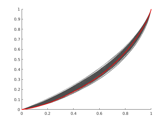
We plot the base case in red, and all others in light gray. We observe that the base case is worse than the average, as the deviation from a piston-like displacement is large.

figure; hold on
plot(F(:, 2:end), Phi(:, 2:end), 'color', [0.3, 0.3, 0.3])
plot(F(:, 1), Phi(:, 1), 'r', 'linewidth', 2)

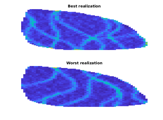
Iterate over all¶

L = zeros(n+1, 1);
for i = 1:n+1
    L(i) = computeLorenz(F(:, i), Phi(:, i));
end

[mv, mix] = min(L);
[Mv, Mix] = max(L);
fprintf('Best case is case #%d with L_c = %1.4f\n', mix, mv);
fprintf('Worst case is case #%d with L_c = %1.4f\n', Mix, Mv);

clf;
subplot(2, 1, 1)
plotCellData(G, rock_all{mix}.perm(:, 1), 'EdgeColor', 'none')
axis tight off
title('Best realization')

subplot(2, 1, 2)
plotCellData(G, rock_all{Mix}.perm(:, 1), 'EdgeColor', 'none')
axis tight off
title('Worst realization')

Best case is case #16 with L_c = 0.2657
Worst case is case #99 with L_c = 0.4118

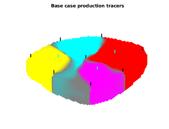
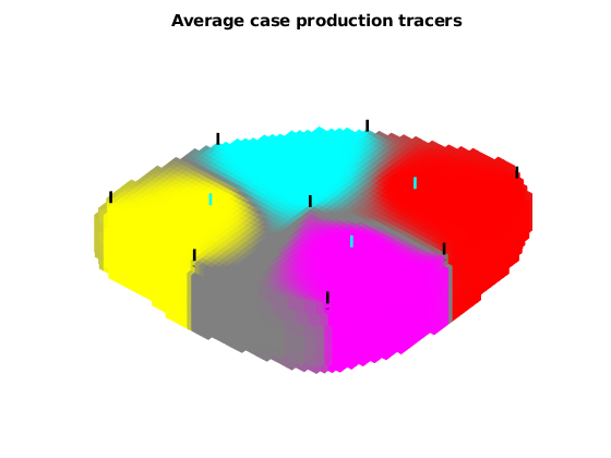
Plot the producer tracer concentrations¶

We plot both the base case, and the averaged case where the tracer value is equal to the average over all realizations. The uncertain regions that change between different wells over the ensamble are colored in gray.

wsign = [W.sign];
figure;
plotTracerBlend(G, D.ppart, max(D.ptracer, [], 2))
title('Base case production tracers')
view(-50, 70);
axis tight off
plotWell(G, W(wsign > 0), 'fontsize', 0, 'color', 'k')
plotWell(G, W(wsign < 0), 'fontsize', 0, 'color', 'c')

figure;
plotTracerBlend(G, ppart, max(ptracer, [], 2))
title('Average case production tracers');
view(-50, 70);
axis tight off
plotWell(G, W(wsign > 0), 'fontsize', 0, 'color', 'k')
plotWell(G, W(wsign < 0), 'fontsize', 0, 'color', 'c')

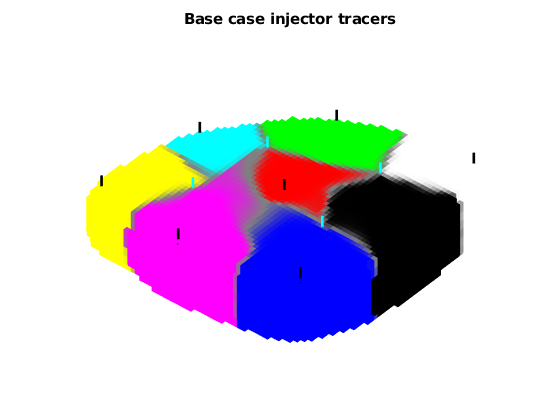
Plot injector tracers¶

figure;
plotTracerBlend(G, D.ipart, max(D.itracer, [], 2))
title('Base case injector tracers');
view(-50, 70);
axis tight off
plotWell(G, W(wsign > 0), 'fontsize', 0, 'color', 'k')
plotWell(G, W(wsign < 0), 'fontsize', 0, 'color', 'c')

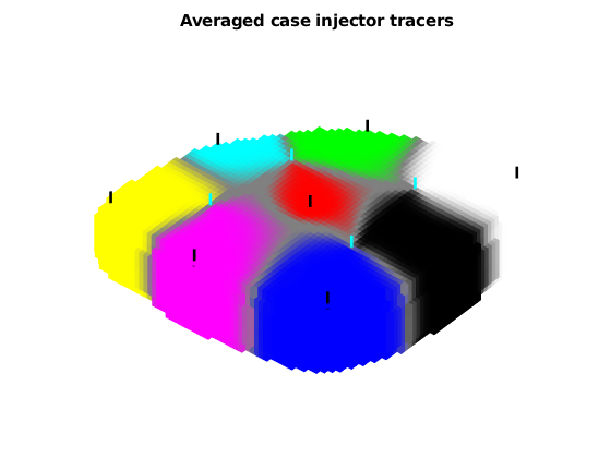
figure;
plotTracerBlend(G, ipart, max(itracer, [], 2))
title('Averaged case injector tracers');
view(-50, 70);
axis tight off
plotWell(G, W(wsign > 0), 'fontsize', 0, 'color', 'k')
plotWell(G, W(wsign < 0), 'fontsize', 0, 'color', 'c')

Flow Pattern and Dynamic Heterogeneity for 2D Five-Spot Problem¶

Generated from diagnostFlowPatterns.m

In this example we will demonstrate how we can use time-of-flight and stationary tracer distribution computed using a standard finite-volume method to visualize flow patterns and compute three different measures for dynamic heterogeneity:

mrstModule add diagnostics spe10 incomp

Set up and solve flow problem¶

As our example, we consider a standard five spot with heterogeneity sampled from Model 2 of the 10th SPE Comparative Solution Project.

[G, W, rock] = getSPE10setup(25);
rock.poro = max(rock.poro, 1e-4);
fluid = initSingleFluid('mu', 1*centi*poise, 'rho', 1014*kilogram/meter^3);
rS = initState(G, W, 0);
T  = computeTrans(G, rock);
rS = incompTPFA(rS, G, T, fluid, 'wells', W);

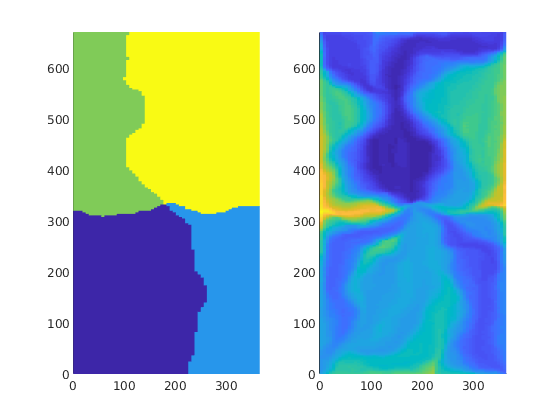
Compute and display time-of-flight and tracer partitioning¶

First we compute time-of-flight which is the travel time from an injector to a given point in the reservoir, and stationary distribution of tracers injected continuously from each injetion well. From the latter, we can easily compute the volume flooded by each injector. Reversing the velocity field, we can cmopute the reverse time-of-flight (the travel time from an arbitrary point to the nearest producer) and the drainage volumes of each producer.

pargs = {'EdgeColor','none'};
D = computeTOFandTracer(rS, G, rock, 'wells', W);
subplot(1,2,1); plotCellData(G,D.ppart,pargs{:}); axis equal tight
subplot(1,2,2); plotCellData(G,log10(sum(D.tof,2)),pargs{:}); axis equal tight

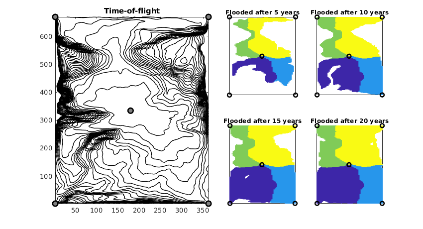
Threshold the tracer regions using time-of-flight to show the development of flooded regions

figure('Position',[600 360 840 460]);
subplot(2,4,[1 2 5 6]);
hold on
contour(reshape(G.cells.centroids(:,1),G.cartDims), ...
              reshape(G.cells.centroids(:,2),G.cartDims), ...
              reshape(D.tof(:,1)/year,G.cartDims),1:25,...
          'LineWidth',1,'Color','k');
xw = G.cells.centroids(vertcat(W.cells),:);
plot(xw(:,1), xw(:,2), 'ok',...
    'LineWidth',2,'MarkerSize',8,'MarkerFaceColor',[.5 .5 .5])
hold off, box on, axis tight, cpos = [3 4 7 8];
title('Time-of-flight');

for i=1:4
   subplot(2,4,cpos(i)); cla
   plotCellData(G,D.ppart, D.tof(:,1)<5*i*year,pargs{:});
   hold on, plot(xw(:,1),xw(:,2),'ok','LineWidth',2)
   title(['Flooded after ' num2str(i*5) ' years']);
   axis tight, box on
   set(gca,'XTick',[],'YTick',[]);
end

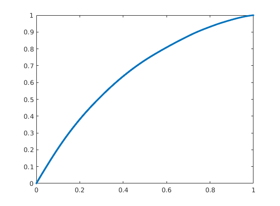
Compute and display flow-capacity/storage-capacity diagram¶

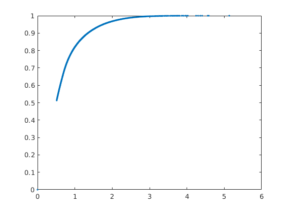
Making an analogue to 1D displacement theory, the F-Phi curve is the equivalent to a plot of the fractional flow versus saturation.

[F,Phi] = computeFandPhi(poreVolume(G,rock),D.tof);
figure, plot(Phi,F,'.');

Compute the Lorenz coefficient¶

The Lorenz coefficient is a popular measure of heterogeneity. It is equal to twice the area under the curve and above the F=Phi line. It varies between 0 (homogeneous displacement) to 1 (infinitely heterogeneous displacement).

fprintf(1, 'Lorenz coefficient: %f\n', computeLorenz(F,Phi));

Lorenz coefficient: 0.317012

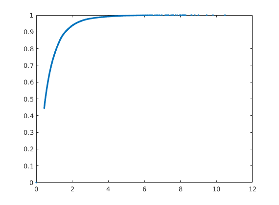
Compute and display sweep efficiency versus dimensionless time¶

Analogue: 1D displacement using the F-Phi curve as a flux function

[Ev,tD] = computeSweep(F,Phi);
figure, plot(tD,Ev,'.');

Copyright notice¶

<html>
% <p><font size="-1

Introduction to Flow Diagnostics¶

Generated from diagnostIntro.m

In this tutorial, we will introduce you to the basic ideas of flow diagnostics. The basic quantitites in flow diagnostics are time-of-flight and numerical tracer partitions, which in turn can be used to compute volumetric connections, flux allocation between wells, and measures of dynamic heterogeneity, or just be used to indicate how displacement fronts will propagate in the reservoir, given a steady flow field. Flow diagnostics has often been associated with streamline methods. Herein, however, we will compute the same kind of quantities and measures using the first-order, finite-volume discretization which is used in MRST and in most commercial reservoir simulators. This means that whereas the computed flow diagnostics may not necessarily be an accurate representation of the corresponding continuous problem, it will represent the volumetric connections and dynamic heterogeneity, as seen by a multiphase simulator. Suggested reading:

mrstModule add diagnostics incomp streamlines;

% NB: In this example, we use the |parula| colormap. If this is not yet
% available in your MATLAB, you can e.g., replace all occurences of
% |parula| with |jet|
pargs = {'EdgeColor','none','FaceAlpha',.6};

Set up and solve flow problem¶

To illustrate the various concepts, we use a rectangular reservoir with five wells, two injectors an five producers

% Grid
[nx,ny] = deal(64);
G = cartGrid([nx,ny,1],[500,250,10]);
G = computeGeometry(G);

% Petrophysical data
p = gaussianField(G.cartDims(1:2), [0.2 0.4], [11 3], 2.5);
K = p.^3.*(1.5e-5)^2./(0.81*72*(1-p).^2);

rock = makeRock(G, K(:), p(:));

hT  = computeTrans(G, rock);
pv  = sum(poreVolume(G,rock));

% Fluid model
gravity reset off
fluid = initSingleFluid('mu', 1*centi*poise, 'rho', 1014*kilogram/meter^3);

% Wells
n = 12;
W = addWell([],  G, rock, nx*n+n+1, ...
    'Type', 'rate', 'Comp_i', 1, 'name', 'I1', 'Val', pv/2);
W = addWell(W, G, rock, nx*n+n+1+nx-2*n, ...
    'Type','rate',  'Comp_i', 1, 'name', 'I2', 'Val', pv/2);
W = addWell(W, G, rock, round(G.cells.num-(n/2-.5)*nx-.3*nx), ...
    'Type','rate',  'Comp_i', 0, 'name', 'P1', 'Val', -pv/4);
W = addWell(W, G, rock, G.cells.num-(n-.5)*nx, ...
    'Type','rate',  'Comp_i', 0, 'name', 'P2', 'Val', -pv/2);
W = addWell(W, G, rock, round(G.cells.num-(n/2-.5)*nx+.3*nx), ...
    'Type','rate',  'Comp_i', 0, 'name', 'P3', 'Val', -pv/4);

% Initial reservoir state
state = initState(G, W, 0.0, 1.0);

Compute basic quantities¶

To compute the basic quantities, we need a flow field, which we obtain by solving a single-phase flow problem. Using this flow field, we can compute time-of-flight and numerical tracer partitions. For comparison, we will also tracer streamlines in the same flow field.

state = incompTPFA(state, G, hT, fluid, 'wells', W);
D = computeTOFandTracer(state, G, rock, 'wells', W);

% Trace streamlines
seed = (nx*ny/2 + (1:nx)).';
Sf = pollock(G, state, seed, 'substeps', 1);
Sb = pollock(G, state, seed, 'substeps', 1, 'reverse', true);

Warning: Well rates and flux bc must sum up to 0
when there are no bhp constrained wells or pressure bc.Results may not be
reliable.

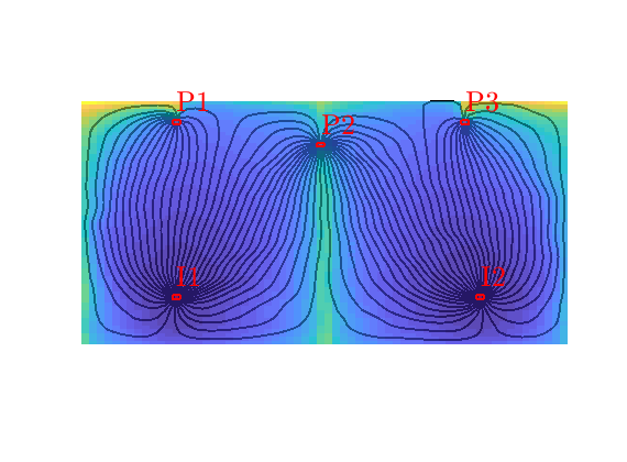
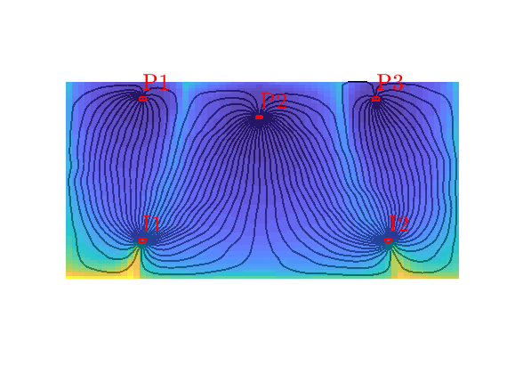
Forward time-of-flight¶

The time-of-flight gives the time it takes a neutral particle to travel from the nearest inflow boundary (e.g., an injection well) and to a given point in the reservoir. Here, we do not compute this quantity pointwise, but rather in an volume-averaged manner over each grid cell

clf
hf=streamline(Sf);
hb=streamline(Sb);
plotGrid(G,vertcat(W.cells),'FaceColor','none','EdgeColor','r','LineWidth',1.5);
plotWell(G,W,'FontSize',20);
set([hf; hb],'Color','w','LineWidth',1.5);
hd=plotCellData(G,D.tof(:,1),pargs{:});
colormap(parula(32));
axis equal off;

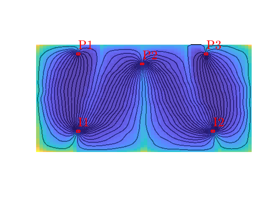
Backward time-of-flight¶

Backward time-of-flight is defined analogously, as the name suggests, by tracing particles backward along the flow field from the nearest outlet (e.g., a production well). For a given point, this quantity thus represents the time it will take a neutral particle to reach the outlet.

delete(hd);
hd=plotCellData(G,D.tof(:,2),pargs{:});

Residence time¶

The residence time is defined as the sum of the forward and backward time-of-flight and gives the total travel time from inlet to outlet. This quantity can be used to distinguish high-flow zones, which have small residence time, from low-flow and stagnation zones, which have high residence times.

delete(hd);
hd=plotCellData(G,sum(D.tof,2),pargs{:});

Tracer from I1¶

Numerical tracer partitions can be thought of as an imaginary paiting experiment, in which we inject a massless, nondiffusive ink of a unique color at each fluid source. At time infinity, each point in the reservoir must then have been colored. If a point receives more than one tracer, the tracer concentrations represent the fractional flow of past each points. The result is a volumetric partition of unity for the reservoir. To illustrate, let us look at the tracer concentration of injector I1, which is one in all parts of the reservoir except near the flow divide, where cells are affected by flow from both injectors.

delete(hd);
t = D.itracer(:,1);
hd = plotCellData(G, t, t>1e-6, pargs{:});

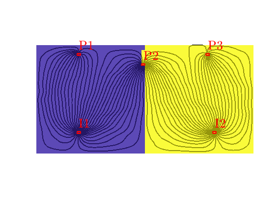
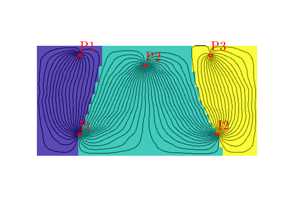
Flooded regions¶

Using this injection tracer, we can define the flooded regions. Each inejctor will influence all cells having a positive tracer concentration. In many cases, however, it is interesting to determine the injector that influences the most. In MRST, this is done by a simple majority vote over all tracers. In lack of a better name, this will be referred to as ‘flood regions’

delete(hd);
hd = plotCellData(G,D.ipart,pargs{:});

Tracer from P2¶

By reversing the flow field, we can compute a similar partition of unity associated with the producers, here illustrated for P2, In the figure, we see that P2 has a region in the middle of the domain that it drains all by itself, whereas the regions to the east and west are also drained by P3 and P1

delete(hd);
t = D.ptracer(:,2);
hd = plotCellData(G, t, t>1e-6, pargs{:});

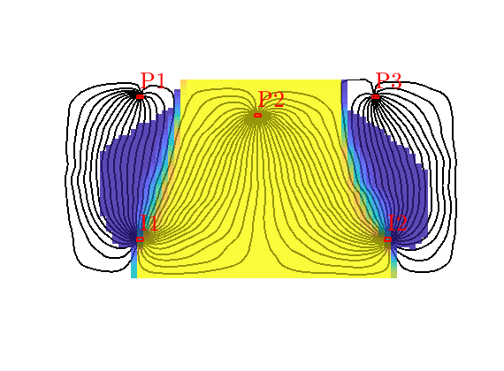
Drainage regions¶

Like we associated flood regions with injectors, we can associate drainage regions with producers, using a simple majority vote over all tracer concentrations

delete(hd);
hd = plotCellData(G,D.ppart,pargs{:});

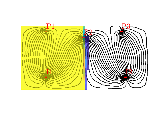
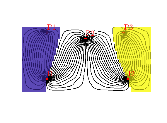
Well regions: I1<->P1, I2<->P3¶

By combining the drainage and flood regions, we can get regions that are affected by a single injector-producer pair

delete(hd);
hd = plotCellData(G,D.ipart, D.ppart~=2, pargs{:});

Compute time-of-flights inside each well region¶

If a cell is affected by more than one injector (or producer), the volume averaged time-of-flight can be very inaccurate as a pointwise measure if the travel times from the two injectors are very different. To amend this, we can compute time of flight for each well

T = computeTimeOfFlight(state, G, rock, 'wells', W, ...
    'tracer',{W(D.inj).cells},'computeWellTOFs', true);

F-Phi diagram¶

To define a measure of dynamic heterogeneity, we can think of the reservoir as a bundle of non-coummunicating volumetric flow paths (streamtubes) that each has a volume, a flow rate, and a residence time. For a given time, the storage capacity Phi, is the fraction of flow paths in which fluids have reached the outlet, whereas F represent the corresponding fractional flow. Both are monotone functions of residence time, and by plotting F versus Phi, we can get a visual picture of the dynamic heterogeneity of the problem. In a completely homogeneous displacement, all flowpaths will break through at the same time and hence F(Phi) is a straight line from (0,0) to (1,1). In a heterogeneous displacement, F(Phi) will be a concave function in which the steep initial slope corresponds to high-flow regions giving early breakthrough and, whereas the flat trailing tail corresponds to low-flow and stagnant regions that would only break through after very long time

[F,Phi] = computeFandPhi(poreVolume(G,rock), D.tof);
clf, plot(Phi,F,'.',[0 1],[0 1],'--');

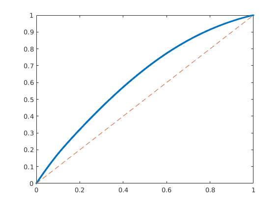
Lorenz coefficient¶

The further the F(Phi) curve is from a straight line, the larger the difference between fast and slow flow paths. The Lorenz coefficient measures the dynamic heterogeneity as two times the area between F(Phi) and the straight line F=Phi.

computeLorenz(F,Phi)

ans =

    0.2437

Sweep effciency diagram¶

We can also define measures of sweep efficiency that tell how effective injected fluids are being used. The volumetric sweep efficiency Ev is defined as the ratio of the volume that has been contacted by the displacing fluid at time t and the volume contacted at infinite time. This quantity is usually related to dimensionless time td=dPhi/dF

[Ev,tD] = computeSweep(F,Phi);
clf, plot(tD,Ev,'.');

Copyright notice¶

<html>
% <p><font size="-1

Optimizing Well Placement and Rates¶

Generated from diagnostOptimWellPlacement.m

This tutorial shows algorithms for optimized well placement and/or optimization of injection rates for regular Cartesian grids. The script optimizes the wells and then runs incompressible simulations with different fluid properties to evaluate the validity of the optimization. Depending on the configuration, this example may take some time to run. Different options can be changed for different results. The default is to optimize the placement of the wells, but not their rates.

mrstModule add ad-core ad-props diagnostics spe10 incomp
close all

Parameters that determine the setup¶

fiveSpotWells = true;          % If false: all injectors near the middle
optimizeSubsteps = true;       % If false: rates not optimized for each step
optimizePlacement = true;      % If false: only iinjection rates optimized
wradius = 5;                   % Search radius for well movement. Larger
                               % values may give faster convergence
rocktype = 'tarbert';          % Values: 'tarbert', 'ness', 'uniform'
[Nx,Ny,Nz] = deal(60,60,1);    % Grid size. SPE: Nx<=60, Ny<=220

switch lower(rocktype)
   case 'ness',
       [offset, uniformRock] = deal(65, false);
   case 'tarbert',
       [offset, uniformRock] = deal(0 , false);
   case 'uniform',
       [offset, uniformRock] = deal(0 , true );
       [optimizeSubsteps,fiveSpotWells,wradius] = deal(false,false,1);
   otherwise
      error('Unknown setup!')
end

Set up reservoir and fluid properties¶

This code is a bit verbose because it allows for different options in the same example.

% Grid setup
G = cartGrid([Nx, Ny, Nz], [Nx, Ny, Nz].*[20, 10, 2].*ft);
G = computeGeometry(G);

% Rock setup
if uniformRock
    rock.poro = repmat(0.3,             [G.cells.num, 1]);
    rock.perm = repmat(100*milli*darcy, [G.cells.num, 1]);
else
    rock = getSPE10rock(1:Nx, 1:Ny, (1:Nz) + offset);
    rock.poro(rock.poro < 0.01) = 0.01;
end
pv = poreVolume(G, rock);
T = computeTrans(G, rock);

% State

% Fluid
fluid_ad = initSimpleADIFluid('mu', [1,1,1].*centi*poise, 'n', [1,1,1]);

% Build discrete operators
ops = setupOperatorsTPFA(G, rock);

Set up wells¶

The wells are set to inject one pore volume per injector over a total period of ten years. We use the array targets to keep track of the wells whose rates are to be optimized. If fiveSpotWells is true, the injectors are set in the corners of the domain. Otherwise, they are positioned ten cells away from the producer.

inRate  = sum(pv)/(10*year);                     % Initial rate
minRate = inRate/4;                              % Minimum allowed rate
[midx, midy] = deal(ceil(Nx/2), ceil(Ny/2));     % Midpoint: producer
addw =  @(W, i, j, k) ...
    verticalWell(W, G, rock, i, j, k, 'Val', inRate, 'Type', 'rate');
W = [];
for i = -1:2:1
   for j = -1:2:1
      if fiveSpotWells
         % Set up injector in each corner
         W = addw(W, Nx*(i==1) + 1*(i==-1), Ny*(j==1) + 1*(j==-1), []);
      else
         % Set up injectors jumbled around the producer
         W = addw(W, midx - 10*i, midy - 10*j, []);
      end
   end
end
targets = 1:numel(W);                   % Indices of wells to be optimized
W = [W; verticalWell([], G, rock, midx, midy, [], ...
                     'Val', 0, 'Type', 'bhp', 'Name', 'P')];

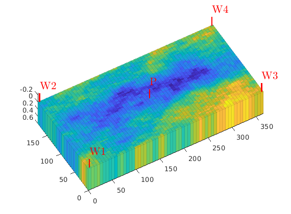
Plot the initial setup¶

clf
plotCellData(G, log10(rock.perm(:, 1)), 'EdgeAlpha', 0.125);
plotWell(G, W, 'height',.25);
axis tight, set(gca,'DataAspect',[1 1 .01]), view(-30,50)

_images/diagnostOptimWellPlacement_01.png

Set up objective functions and optimize¶

As objective function for the optimization, we will use the Lorenz coefficient, which means that we try to equilibrate the length of all flow paths. The optimization may take some time if both rates and placement are to be optimized.

% Objective function
objective = getObjectiveDiagnostics(G, rock, 'minlorenz');

% Handle for pressure solver
state0 = initResSol(G, 0*barsa, [0 1 0]);
solvePressure = @(W, varargin) ...
   solveStationaryPressure(G, state0, ops, W, fluid_ad, pv, T, ...
   'objective', objective, varargin{:});

% Solve pressure and display objective value
[state, D, grad0] = solvePressure(W); grad0.objective.val

% Optimize
if optimizePlacement
    [W_opt, wellHistory, optHistory] = ...
        optimizeWellPlacementDiagnostics(G, W, rock, objective, targets, ...
               D, minRate, state0, fluid_ad, pv,T, ops, ...
               'optimizesubsteps', optimizeSubsteps, ...
               'searchRadius', wradius, 'wellSteps', 1, ...
               'plotProgress', true);
    [state_o, D_best, grad] = ...
        solvePressure(W_opt, 'linsolve', @mldivide);
else
    [D_best, W_best, history] = ...
        optimizeTOF(G, W, fluid_ad, pv, T, ops,state0, minRate, ...
               objective, 'targets', targets, 'plotProgress', true); %#ok<UNRCH>
    wellHistory = [];
end

ans =

    0.3129

Optimizing well 1...
Improved value, 0.218 to 0.181
Optimizing well 2...
...

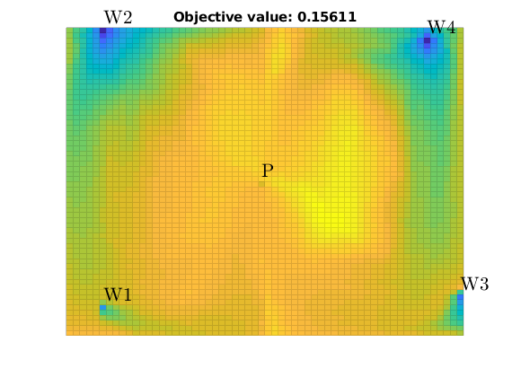
_images/diagnostOptimWellPlacement_02.png

Plot well paths¶

We plot the paths taken by the well placement algorithm. This will only plot the porosity if only the injection rates is optimized.

clf, hold on
if uniformRock, ec = 'k'; else ec = 'none'; end
plotCellData(G, rock.poro, 'FaceAlpha', 1, 'EdgeColor', ec, 'EdgeAlpha', 0.1)
gc = G.cells.centroids;
colors = {'r', 'w', 'b', 'm'};
for i = 1:numel(targets)
    v = W(targets(i)).cells;
    for j = 1:numel(wellHistory), v = [v; wellHistory{j}(i).visited]; end  %#ok<AGROW>

    plot3(gc(v, 1), gc(v, 2), -ones(numel(v), 1), ...
          ['o--', colors{i}], 'LineWidth', 2, 'MarkerSize', 10, ...
          'MarkerEdgeColor', 'black', 'MarkerFaceColor', colors{i})
end
axis tight equal off
view(0, 89.9)
pc = W_opt(end).cells;
plot3(gc(pc, 1), gc(pc, 2), -ones(numel(v), 1), ['o--', 'w'], ...
      'LineWidth', 2, 'MarkerSize', 10, 'MarkerEdgeColor', 'black', ...
      'MarkerFaceColor', 'w')
plot3(gc([W_opt.cells], 1), gc([W_opt.cells], 2), ...
      -ones(numel([W_opt.cells]), 1), ['X', colors{i}], 'LineWidth', 2, ...
      'MarkerSize', 10, 'MarkerEdgeColor', 'black', ...
      'MarkerFaceColor', colors{i})

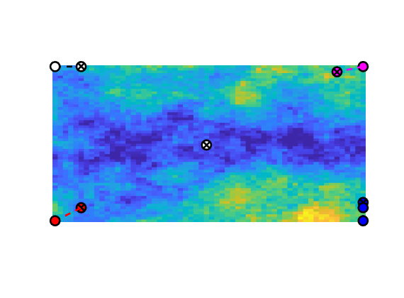
_images/diagnostOptimWellPlacement_03.png

Plot total travel time for both base and optimized case¶

We plot the total travel time (sum of backward and forward time of flight) for both the initial and the optimized configuration. To ensure that the improvement can be seen, the colorbars are scaled by the base case. If the optimization was successful, the regions with very high total time of flight that corresponding to poor sweep should be reduced. The highest travel time is colorized dark red.

clear cx, close all
Wells = {W, W_opt};
WellNames = {'Original', 'Optimized placement'};
[Phis, Fs] = deal([]);
clf
for i = 1:numel(Wells)
    [state, Dx, gradpost] = solvePressure(Wells{i});
    [F, Phi] = computeFandPhi(pv, Dx.tof);
    Lc = computeLorenz(F, Phi);

    subplot(2,1, i)
    plotCellData(G, log10(sum(Dx.tof, 2)), 'EdgeColor','none')
    if exist('cx', 'var'), caxis(cx), else cx = caxis();end
    title(sprintf('%s, L_c = %1.2f', WellNames{i}, Lc))
    plotWellsPrint(G, Wells{i}, D)
    axis tight off; colorbar

    Phis = [Phis, Phi];                                         %#ok<AGROW>
    Fs = [Fs, F];                                               %#ok<AGROW>
end
% Add the baseline optimal case (i.e., a linear function of Phi)
Phis = [Phis, Phi];
Fs = [Fs, Phi];

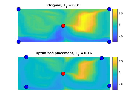
_images/diagnostOptimWellPlacement_04.png

Plot the storage / flow capacity diagrams¶

We also plot the flow capacity / storage capacity diagram (F-Phi) curves for both the base and optimized case. As the Lorenz’ coefficient is defined proportionally to the integral between the idealized curve and actual curve, the improvement is easy to see from the resulting plot.

figure;
plot(Phis, Fs, '--', 'LineWidth', 2)
if fiveSpotWells
    fs = 'Five spot';
else
    fs = 'Initial well placement';
end
title('F / Phi-curve before and after optimization');
xlabel('\Phi');
ylabel('F');
grid on
legend({fs, 'Improved well placement', 'Idealized displacement'}, ...
       'location', 'South')

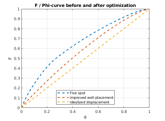
_images/diagnostOptimWellPlacement_05.png

Run two-phase simulation to validate the results¶

To validate that the optimization correlates with the simulated oil recovery, we simulate a five year period using two different fluids. The first fluid model has idential properties for both phases effectively giving us a red/blue-water problem that should give very good oil recovery even for the base case, as the saturation fronts will be sharp and the water will displace the “oil” efficiently. The second fluid model has a significant viscosity ratio of 10, which makes oil recovery much more challenging because the displacing fluid will tend to finger through the resident fluid. The purpose of this setup is to validate that the single-phase optimization procedure still has merit when extended to multiphase problems. For simplicity, the problem is incompressible and uses a pressure/transport splitting for speed.

% Define recovery via pore volume
recov = @(state) 1 - sum(state.s(:,2).*pv)/sum(pv);
close all

% Make a copy of the wells, and explicitly make them two-phase wells.
W_initial = W;
W_improved = W_opt;
for i = 1:numel(W_initial)
    W_initial(i).compi = W_initial(i).compi(1:2);
    W_improved(i).compi = W_improved(i).compi(1:2);
end

% Set up fluids
fluids = cell([2, 1]);
fluids{1} = initSimpleFluid('mu' , [   1,    1]*centi*poise     , ...
                            'rho', [1000, 1000]*kilogram/meter^3, ...
                            'n'  , [   1,    1]);
fluids{1}.name = 'unitary';

fluids{2} = initSimpleFluid('mu' , [   1,  10]*centi*poise     , ...
                            'rho', [1000, 700]*kilogram/meter^3, ...
                            'n'  , [   1,   1]);
fluids{2}.name = 'oil-water';

% Store the different states in cell arrays
states_improved = cell(2,1);
states_initial = cell(2,1);

for i = 1:numel(fluids)
    h = figure;
    fluid = fluids{i};
    state_a = state0;
    state_a.s = state_a.s(:,1:2);
    state_b = state_a;

    initial = [];
    improved = [];

    % Pressure solve - TPFA discretization
    psolve = @(state, w) ...
       incompTPFA(state, G, T, fluid, 'wells', w, 'Verbose', false);

    % Transport solve - implicit transport solver
    tsolve = @(state, w, dT) ...
       implicitTransport(state, G, dT, rock, fluid, ...
                         'wells', w, 'Verbose', false);

    % Make convenient function handle for doing both pressure and
    % transport
    solve = @(state, w, dT) tsolve(psolve(state, w), w, dT);

    % Five day timesteps to get a nice animation
    dt = 5*day;
    Time = 0;
    % Five year horizont

    endtime = 5*year;
    ntschar = numel(formatTimeRange(endtime - dt));
    while Time < endtime
        % Solve the timestep and store the data
        state_a = solve(state_a, W_initial, dt);
        state_b = solve(state_b, W_improved, dt);

        initial = [initial; state_a]; %#ok
        improved = [improved; state_b]; %#ok
        Time = Time + dt;
        sa = state_a.s(:,2);
        sb = state_b.s(:,2);

        % Plot the base case
        set(0, 'CurrentFigure', h);
        subplot(2,2,1), cla
        plotCellData(G, sa, 'EdgeAlpha', 0.125);
        title('Oil saturation, base case')
        caxis([0, 1]), axis tight off

        % Plot the improved case
        subplot(2,2,2), cla
        plotCellData(G, sb, 'EdgeAlpha', 0.125);
        title('Oil saturation, optimized')
        caxis([0, 1]), axis tight off

        % Plot the historic oil production underway
        subplot(2,2, 3:4), cla
        plot(convertTo(cumsum(repmat(dt, [numel(initial), 1])), year), ...
            100*arrayfun(recov, [initial, improved]), '-', 'LineWidth', 2)
        xlim([0, endtime/year]), ylim([0, 100]);
        grid on
        xlabel('Years'), ylabel('Oil recovered (%)')
        legend('Base case', 'Optimized', 'location', 'southeast')
        title(['Recovery for ', fluid.name, ' fluid']);
        drawnow

        % Ouput to terminal...
        fprintf(['Recovery after %-*s: ', ...
                 'Initial: %4.1f%%, Modified: %4.1f%%\n'],  ...
                 ntschar, formatTimeRange(Time), ...
                 100*recov(state_a), ...
                 100*recov(state_b))
    end

    states_initial{i} = initial;
    states_improved{i} = improved;
end

Recovery after 5 Days           : Initial:  0.5%, Modified:  0.5%
Recovery after 10 Days          : Initial:  1.1%, Modified:  1.1%
Recovery after 15 Days          : Initial:  1.6%, Modified:  1.6%
Recovery after 20 Days          : Initial:  2.2%, Modified:  2.2%
Recovery after 25 Days          : Initial:  2.7%, Modified:  2.7%
Recovery after 30 Days          : Initial:  3.3%, Modified:  3.3%
Recovery after 35 Days          : Initial:  3.8%, Modified:  3.8%
Recovery after 40 Days          : Initial:  4.4%, Modified:  4.4%
...

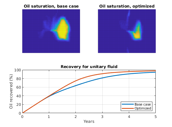
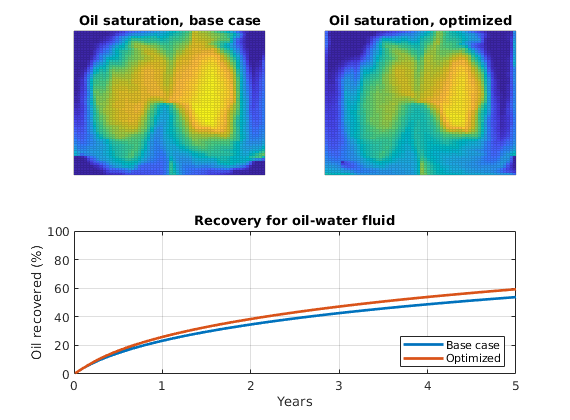
_images/diagnostOptimWellPlacement_06.png

_images/diagnostOptimWellPlacement_07.png

Plot the recovery at the half-way point¶

If we simulate long enough, almost all oil will certainly be recovered. We plot the half-way point after 2.5 years to show the oil saturation along with the well positions.

clf
ind = round(2.5*year/dt);

nr = numel(states_initial);
for i = 1:nr
    initial = states_initial{i};
    improved = states_improved{i};
    sa = initial(ind).s(:,2);
    sb = improved(ind).s(:,2);

    subplot(2, nr, 1 + (i-1)*nr)
    plotCellData(G, sa, 'EdgeColor', 'none')
    plotWellsPrint(G, W, D)
    view(0, 89);
    title(sprintf('Recovery baseline, %s: %4.1f%%', ...
                  fluids{i}.name, 100 * recov(initial(ind))))
    axis tight off
    colorbar
    caxis([0, 1])

    subplot(2, nr, 2 + (i-1)*nr)
    plotCellData(G, sb, 'EdgeColor', 'none')
    plotWellsPrint(G, W_opt, D)
    view(0, 89);
    title(sprintf('Recovery improved, %s: %4.1f%%', ...
                  fluids{i}.name, 100 * recov(improved(ind))))
    colorbar
    caxis([0, 1])

    axis tight off
end

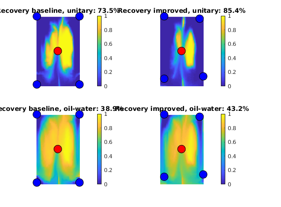
_images/diagnostOptimWellPlacement_08.png

Plot both problems in the same plot¶

We plot the oil recovery for both fluid problems simultanously, showing that the optimized placement improves recovery in either case. The effect on oil recovery from viscosity differences is also shown to be significant.

figure
t = convertTo(cumsum(repmat(dt, [numel(states_initial{1}), 1])), year);
y = [states_initial{1}, states_initial{2}, ...
     states_improved{1}, states_improved{2}];
plot(t, 100*arrayfun(recov, y), 'LineWidth', 2)
grid on
xlabel('Years')
ylabel('Oil recovery (%)')
legend('Five spot, unit fluids',       ...
       'Five spot, oil/water',         ...
       'Optimized wells, unit fluids', ...
       'Optimized wells, oil/water',   ...
       'Location', 'SouthEast')

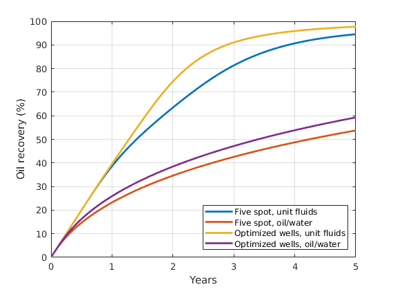
_images/diagnostOptimWellPlacement_09.png

Copyright notice¶

<html>
% <p><font size="-1

Well Optimization using Adjoints and Flow Diagnostics¶

Generated from diagnostOptimize1D.m

This example demonstrates the diagnostics-based well optimization framework on a very simple 1D problem with two injectors and a single producer.

mrstModule add diagnostics ad-props incomp ad-core

Setup model¶

We consider a rectangular 10-by-1-by-1 m^3 discretized into 101 cells. We divide the reservoir into two regions: One region (x<5) where the porosity is set to 0.5 and a region x>5 where the porosity is 1. In the center (x = 5), the porosity is set to the average (0.75). Two injectors are defined. One at the left boundary of the domain and another at the right end of the domain. Both are allocated the same injection rate, even though they are in different porosity regions. A single BHP controlled producer is placed in the exact middle of the domain, effectively making the reservoir into two distinct regions: The low porosity region swept by the first injector and the high porosity region swept by the other injector.

% Grid
N = 101; mid = floor(N/2);
G = cartGrid([N, 1, 1], [10, 1, 1]);
G = computeGeometry(G);

% Petrophysics
[lowporo,highporo] = deal(.5,1);
poro = ones(G.cells.num, 1);
poro(1:mid) = lowporo;                 % West part of reservoir
poro(mid+1:end) = highporo;            % East part of reservoir
poro(mid) = (lowporo + highporo)/2 ;   % Center cell
rock = makeRock(G, 1, poro);

T = computeTrans(G, rock);
pv = poreVolume(G, rock);

% Wells
W = verticalWell([], G, rock, 1, 1, [],  ...
 % Injector: West
                 'Val', 1*meter^3/day, 'Type', 'rate', ...
                 'Name', 'I1', 'InnerProduct', 'ip_tpf');

W = verticalWell(W, G, rock, N, 1, [], ...
   % Injector: East
                 'Val', 1*meter^3/day,  'Type', 'rate', ...
                 'Name', 'I2', 'InnerProduct', 'ip_tpf');

W = verticalWell(W, G, rock, mid, 1, [], ...
 % Producer: Center
                 'Val', 0, 'Type', 'bhp', ...
                 'Name', 'P', 'InnerProduct', 'ip_tpf');

% Reservoir state
state0 = initResSol(G, 0*barsa, [1 0 0]);
% state0.wellSol = initWellSol(W, 0);

% Reservoir fluid
fluid_ad = initSimpleADIFluid('mu',[1 1 1], 'n', [1 1 1]);

% Set up discrete operators
op = setupOperatorsTPFA(G, rock);

Define objective function and plot domain¶

The Lorenz coefficient is used here, which will have values between 0 (homogenous displacement, perfect sweep) and 1 (infinitely hetereogenous displacement). Because we want to improve the sweep of the well configuration, this is a good choice. The left injector has half the pore volume between it and the producer when compared to the other injector, and so the optimal configuration should set the ratio between the injectors’ rates to 1/2. We at the same time specify the minimum rates per well to a small value, which will not be violated at the optimum in this simple case. Once the problem definition is complete we plot the wells and porosity on the 1D domain.

objective = getObjectiveDiagnostics(G, rock, 'minlorenz');

minRate = W(1).val./1000;
clf
x = G.cells.centroids(:,1);
stairs(x, rock.poro, '-k', 'LineWidth', 2);
grid on
ylim([0, 1.1])
hold on
colors = {'r', 'g', 'b'};
% Plot each well
for i = 1:numel(W)
    c = W(i).cells(1);
    plot(x(c, 1), rock.poro(c), 'O', 'MarkerEdgeColor', 'k', ...
                    'MarkerFaceColor', colors{i}, 'MarkerSize', 8);
end
l = {'Porosity', W.name };
legend(l, 'location', 'southeast')
title('Porosity and well placements')
ylabel('Porosity')
xlabel('X coordinates')

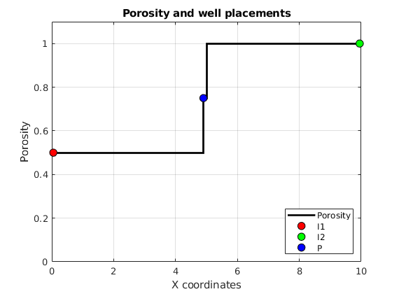
Optimize well rates¶

We optimize the well rates using a steepest descent-like implementation which accounts for well limits and uses adjoints to calculate the sensitivites of the objective function. Because the framework uses diagnostics for the objective evaluations and adjoints for the sensitivities, the cost per function evaluation is low. We set the tolerance so the iteration has converged when the change between iterations is less than 5%. During the optimization, the progress will be plotted.

clf
[D_best, W_best, history] = optimizeTOF(G, W, fluid_ad, pv, T, op,...
                                     state0, minRate, objective, ...
                                     'plotProgress', true, ...
                                     'verbose', true, ...
                                     'deltatol', 0.05);

Obj: 0.186937 at initial controls
Obj: 0.336277 (delta: 0.8, alpha: 9e-06) at iteration 0
Obj: 0.336348 (delta: 0.8, alpha: 9e-07) at iteration 1
Obj: 0.336309 (delta: 0.8, alpha: 9e-08) at iteration 2
Obj: 0.336272 (delta: 0.8, alpha: 9e-09) at iteration 3
Obj: 0.336307 (delta: 0.8, alpha: 9e-10) at iteration 4
Obj: 0.113024 (delta: -0.4, alpha: 9e-11) at iteration 5
================ VALUE IMPROVED ==================
...

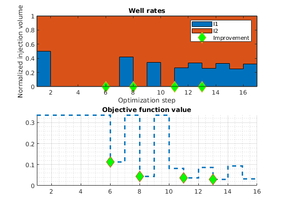
Plot the time of flight of the initial and the best well rates¶

We plot the time of flight in the domain for each configuration. The optimized well configuration shouws equal arrival times from each injector, indicating an optimal solution.

clf
pw = @() plotWell(G, W, 'height', 1, 'radius', 0, 'Color', 'red');

subplot(4,1,1:2), title('Time of flight')
x = G.cells.centroids(:,1);
initial = history.D(1).tof(:,1);
optimized = history.D(end).tof(:,1);
hold on
plot(x, [initial, optimized]./max(initial), 'LineWidth', 2)
grid on
legend({'Initial TOF', 'Optimized TOF'});

subplot(4,1,3), title('Initial')
plotCellData(G, history.D(1).tof(:,1),'EdgeColor','k','EdgeAlpha',.1)
[htop, htext] = pw(); %#ok<ASGLU>
set(htext, 'Interpreter', 'None')
axis normal off
view(-4, 40)

subplot(4,1,4), title('Optimized')
colormap winter
plotCellData(G, history.D(end).tof(:,1),'EdgeColor','k','EdgeAlpha',.1)
[htop, htext] = pw();
set(htext, 'Interpreter', 'None')
axis tight off
view(-4, 40)

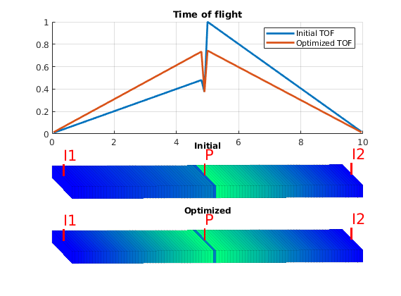
Plot sweep and flow capacity diagrams¶

The Lorenz coefficient is really a derived measure from the flow-capacity diagram, equal to the integral of the deviation from a perfect, linear flow curve where every unit of fluid injected corresponds to a unit of recovery. We compute the F and Phi quantities for the base case and the optimum and plot both. At the same time, we plot the sweep diagrams for the same configurations.

[F_0, Phi_0] = computeFandPhi(pv, history.D(1).tof);
[F_end, Phi_end] = computeFandPhi(pv, history.D(end).tof);

clf;
subplot(2,1,1), title('Flow-capacity diagram')
plot([Phi_0, Phi_end], [F_0, F_end], 'linewidth', 2)
legend({'Equal rates', 'Optimized rates'}, 'location', 'SouthEast')
xlabel('\Phi'), ylabel('F'), grid on

subplot(2,1,2), title('Sweep')
[Ev_0, tD_0] = computeSweep(F_0, Phi_0);
[Ev_end, tD_end] = computeSweep(F_end, Phi_end);
plot([tD_0, tD_end], [Ev_0, Ev_end], 'linewidth', 2)
legend({'Equal rates', 'Optimized rates'}, 'location', 'SouthEast')
xlabel('\Phi'), ylabel('F'), grid on, axis tight

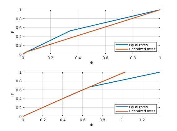
Copyright notice¶

<html>
% <p><font size="-1

Illustrate use of flow diagnostics to verify upscaling¶

Generated from diagnostUpscaleIntro.m

In this example we explain how to use match in cumulative well-allocation factors to verify the quality of an upscaling. In each well completion, the well-allocation factor is the percentage of the flux in/out of the completion that can be attributed to a pair of injection and production wells.

mrstModule add agglom upscaling coarsegrid diagnostics incomp

Make model¶

We make a small model that consists of two different facies with contrasting petrophysical properties. An injector and a producer are placed diagonally oposite of each other and completed mainly in the high-permeable part of the model.

G  = computeGeometry(cartGrid([40 20 15]));
K1 = gaussianField(G.cartDims, [200 2000]);
p1 = K1(:)*1e-4 + .2;
K1 = K1(:)*milli*darcy;
K2 = gaussianField(G.cartDims, [10 500]);
p2 = K2(:)*1e-4 + .2;
K2 = K2(:)*milli*darcy;

rad1 = G.cells.centroids(:,1).^2 + .5*G.cells.centroids(:,2).^2 ...
   + (G.cells.centroids(:,3)-2).^2;
rad2 = .5*(G.cells.centroids(:,1)-40).^2 + 2*G.cells.centroids(:,2).^2 ...
   + 2*(G.cells.centroids(:,3)-2).^2;

ind = ((rad1>600) & (rad1<1500)) | ((rad2>700) & (rad2<1400));
rock = makeRock(G, K2(:), p2(:));
rock.perm(ind) = K1(ind);
rock.perm = bsxfun(@times, rock.perm, [1 1 1]);
rock.poro(ind) = p1(ind);
pv = poreVolume(G, rock);

gravity off

W = verticalWell([], G, rock, 4, 17, 4:15, 'Comp_i', [1, 0], ...
   'Type', 'rate', 'Val', 0.2*sum(pv)/year, 'Name', 'I');
W = verticalWell(W,  G, rock, 35, 3, 1:10, 'Comp_i', [0, 1], ...
   'Type', 'rate', 'Val', -0.2*sum(pv)/year, 'Name', 'P');

figure(1); clf,
set(gcf,'Position', [860 450 840 310],'PaperPositionMode','auto');
subplot(1,2,1);
plotCellData(G,rock.poro,'EdgeAlpha',.5); view(3);
plotWell(G,W,'Color','k'); axis off tight

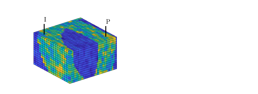
Compute flow on the fine-scale model¶

Transmissibility

hT = computeTrans(G, rock);
trans = 1 ./ accumarray(G.cells.faces(:,1), 1 ./ hT, [G.faces.num, 1]);

% Fluid model
dfluid = initSimpleFluid('mu' , [   1,  10]*centi*poise     , ...
                         'rho', [1014, 859]*kilogram/meter^3, ...
                         'n', [2 2]);
% Pressure solution
xd  = initState(G, W, 100*barsa, [1, 0]);
nw = numel(W);
xd  = incompTPFA(xd, G, trans, dfluid, 'wells', W, 'use_trans', true);

Flow diagnostics on fine-scale model¶

To better reveal the communication in the reservoir, we subdivide each well into two segments, an upper and a lower segments, so that we altogether will have four well-pairs whose well-allocation factors can be used to verify the quality of the upscaling

nsegment=2;
[xd,Wdf] = expandWellCompletions(xd, W,[(1:nw)' repmat(nsegment,nw,1)]);
Df  = computeTOFandTracer(xd, G, rock, 'wells', Wdf);
WPf = computeWellPairs(xd, G, rock, Wdf, Df);

Coarse-scale solution¶

We make a 5x5x15 coarse grid, in which we have chosen to keep the layering of the fine-scale model to simplify the comparison of well-allocation factors. Transmissibilities and well indices are upscaled using two slighly different methods: for the transmissibilities we use global generic boundary conditions and on each coarse face use the solution that has the largest flux orthogonal to the face to compute the upscaled transmissibility. For the wells, we use a specific well conditions and use least squares for the flux.

p  = partitionCartGrid(G.cartDims, [5 5 15]);
CG = coarsenGeometry(generateCoarseGrid(G, p));
[~,CTrans] = upscaleTrans(CG, hT, 'match_method', 'max_flux', ...
                          'bc_method', 'bc_simple');
[~,~,WC]   = upscaleTrans(CG, hT, 'match_method', 'lsq_flux', ...
                          'bc_method', 'wells_simple', 'wells', W);
crock = convertRock2Coarse(G, CG, rock);

figure(1); subplot(1,2,2);
plotCellData(CG,crock.poro);
plotFaces(CG, boundaryFaces(CG),...
   'EdgeColor', [0.4 0.4 0.4],'EdgeAlpha',.5, 'FaceColor', 'none'); view(3);
plotWell(G,W,'Color','k'); axis off tight

xd    = initState(CG, WC, accumarray(p,100*barsa)./accumarray(p,1), [1, 0]);
xd    = incompTPFA(xd, CG, CTrans, dfluid, 'wells', WC, 'use_trans', true);

Warning: Set boundary face trans to zero

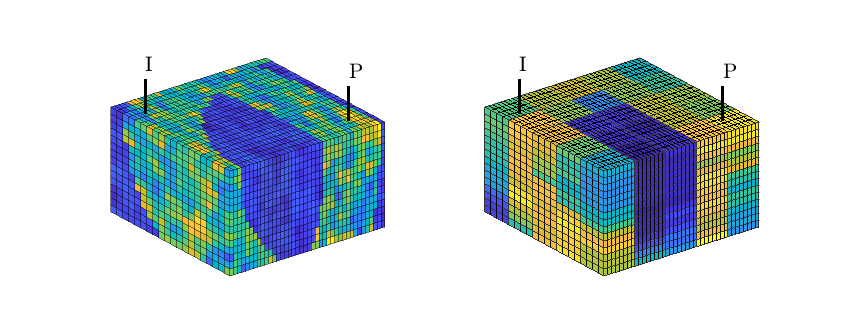
Flow diagnostics on the upscaled model¶

Having obtained fluxes on the coarse model, we can expand the wells into two segments that exactly match the subdivision of in the fine-scale model and compute flow diagnostics.

nw    = numel(WC);
[xdc,Wdc] = expandCoarseWellCompletions(xd, WC, Wdf, p);
Dc    = computeTOFandTracer(xdc, CG, crock, 'wells', Wdc);
WPc   = computeWellPairs(xdc, CG, crock, Wdc, Dc);
nit   = numel(Df.inj);
npt   = numel(Df.prod);
nseg  = nit + npt;

Display bar charts of flow-allocation factors¶

For each well segment, we plot bar chart of the cumulative flux in/out of the completions that make up the segment, from bottom to top. In the plots, each well segment is assigned a unique color and each bar is subdivided into the fraction of the total in/outflux that blongs to the different well-pairs the segment is part of. The plots show the allocation factors for the upper half of the injector (I:1, upper-left plot), the lower part of the injector (I:2, upper-right plot), the upper part of the producer (P:1, lower-left plot), and the lower part of the producer (P:2, lower-right plot). Looking at the bar chart for I:1, we see that the majority of the flux from this injector is colored yellow and hence goes to P:1, which corresponds to the upper part of the producer.

figure(2); set(gcf,'Position', [860 450 840 400]); clf
plotWellAllocationComparison(Dc, WPc, Df, WPf);
dy = [-.05 -.05 -.025 -.025];
dx = [-.5 0 -.5 0 0];
for i=1:4
   subplot(2,2,i);
   pos = get(gca,'Position');
   pos = pos + [-.05 dy(i) .075 .075];
   set(gca,'Position',pos,'XTick',[],'YTick',[]);
end
cmap = jet(nseg); cmap = 0.6*cmap + .4*ones(size(cmap)); colormap(cmap);

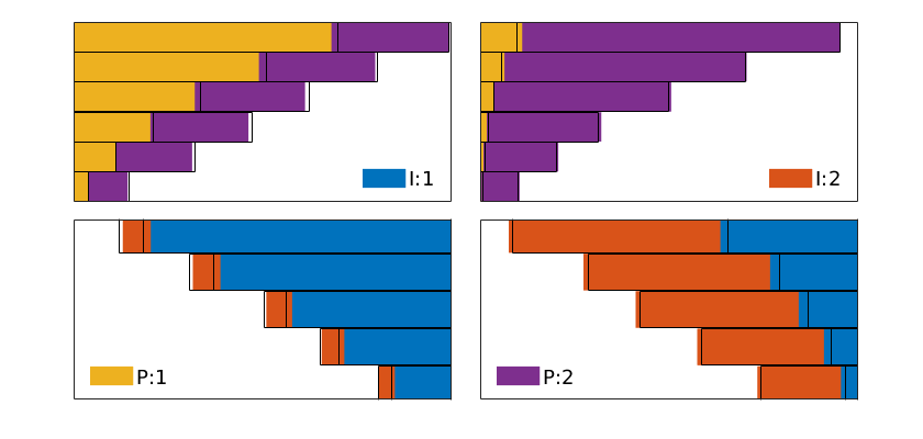
Display the partition¶

Last we show the cells that belong to the four different well segments and show the corresponding injector/producer partitions. We can now compare the partitions with the well-allocation factors in Figure 2. Let us take the allocation for I:2 as an example. In the upper-right plot of Figure 2 we see that almost all the flux from this injector goes to P:2. Looking at the cyan region in the left plot of Figure 1 confirms this: this region is hardly in contact with the yellow segment of the producer. The blue region, on the other hand, contains both the upper segment of the producer (P:1, yellow color) and parts of the lower segment (P:2, red color). Likewise, The red volume in the right-hand plot of Figure 3 covers both the lower segment of the injector (I:2, cyan) and parts of the upper segment (I:1, blue). In the bars of P:2 to the lower-right in Figure 2, we therefore see that relatively large portion of the bars are in blue color.

oG  = computeGeometry(cartGrid([1 1 1],[40 20 15]));
figure(3); clf
set(gcf,'Position', [860 450 840 310],'PaperPositionMode','auto');
subplot(1,2,1);
for i=1:nit
   plotCellData(G,Df.ipart,Df.ipart==i,'FaceAlpha',.3,'EdgeAlpha',.2);
end
plotGrid(oG,'FaceColor','none');
for i=1:nseg,
   plotGrid(G,Wdf(i).cells,'FaceColor',cmap(i,:));
end
plotWell(G,W,'Color','k');
view(-40,10); axis tight off; caxis([1 nit+npt]);

subplot(1,2,2);
for i=1:npt
   plotCellData(G,Df.ppart+nit,Df.ppart==i,'FaceAlpha',.4,'EdgeAlpha',.2);
end
plotGrid(oG,'FaceColor','none');
for i=1:nseg,
   plotGrid(G,Wdf(i).cells,'FaceColor',cmap(i,:));
end
plotWell(G,W,'Color','k');
view(-40,10); axis tight off; caxis([1 nit+npt]);
colormap(cmap);

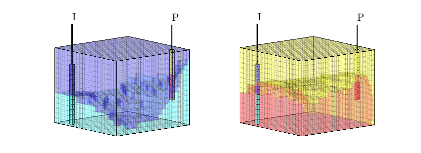
Copyright notice¶

<html>
% <p><font size="-1

Interactive diagnostics on the SAIGUP dataset¶

Generated from diagnostViewerDemo.m

This example sets up interactive diagnostics on a corner point grid. The example uses the same geological dataset as in saigupField1phExample with a number of arbitrary wells. The example is short, as the primary purpose is to create the interactive figures produced by interactiveDiagnostics.

mrstModule add diagnostics mrst-gui incomp

Set up grid and rock¶

grdecl = fullfile(getDatasetPath('SAIGUP'), 'SAIGUP.GRDECL');
grdecl = readGRDECL(grdecl);

actnum        = grdecl.ACTNUM;
grdecl.ACTNUM = ones(prod(grdecl.cartDims),1);
G             = processGRDECL(grdecl, 'checkgrid', false);
G             = computeGeometry(G(1));

rock = grdecl2Rock(grdecl, G.cells.indexMap);
is_pos                = rock.perm(:, 3) > 0;
rock.perm(~is_pos, 3) = min(rock.perm(is_pos, 3));
rock.perm = convertFrom(rock.perm, milli*darcy);

Set up wells¶

The wells are simply placed by a double for loop over the logical indices. The resulting wells give producers along the edges of the domain and injectors near the center.

pv = poreVolume(G, rock);
ijk = gridLogicalIndices(G);
W = [];
gcz = G.cells.centroids;
[pi,ii] = deal(1);
for i = 5:12:G.cartDims(1)
   for j = 5:25:G.cartDims(2)
      c = ijk{1} == i & ijk{2} == j;
      if any(c)
         c = find(c);
         x = gcz(c(1), 1); y = gcz(c(1), 2);
         if x > 500 && x < 2000 && y < 7000 && y > 1000
            % Set up rate controlled injectors for cells in the middle
            % of the domain
            val = sum(pv)/(1000*day);
            type = 'rate';
            name = ['I' num2str(ii)];
            ii = ii + 1;
         else
            % Set up BHP controlled producers at the boundary of the
            % domain
            val = 250*barsa;
            type = 'bhp';
            name = ['P' num2str(pi)];
            pi = pi + 1;
         end
         W = addWell(W, G, rock, c, 'Type', type, 'Val', val, ...
             'Name', name, 'InnerProduct', 'ip_tpf');
      end
   end
end
% Plot the resulting well setup
clf
plotCellData(G, rock.poro,'EdgeColor','k','EdgeAlpha',.1),
plotWell(G, W)
view(-100, 25)

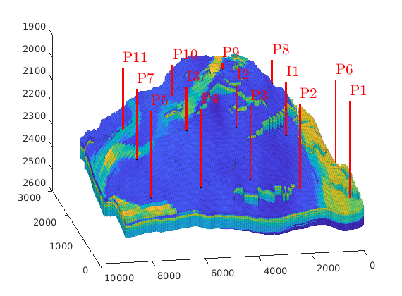
Set up a reservoir state¶

This is not strictly needed for the diagnostics application, but it allows us to see the reservoir component distribution around producers grouped by time of flight. The distribution of phases is done based on a simple hydrostatic approximation by using cell centroids. Some phase mixing is present.

state = initResSol(G, 200*barsa, [0 0 0]);

gcz = G.cells.centroids(:, 3);
height = max(gcz) - min(gcz);
pos = 1 - (gcz - min(gcz))./height;

oil = pos > 0.4 & pos < 0.8;
gas = pos > 0.7;
wat = pos < 0.45;

state.s(wat, 1) = 1;
state.s(oil, 2) = 1;
state.s(gas, 3) = 1;

state.s = bsxfun(@rdivide, state.s, sum(state.s, 2));

clf;
rgb = @(x) x(:, [2 3 1]);
plotCellData(G, rgb(state.s), 'EdgeColor', 'k', 'EdgeAlpha', 0.1)
view(-100, 25)
axis tight

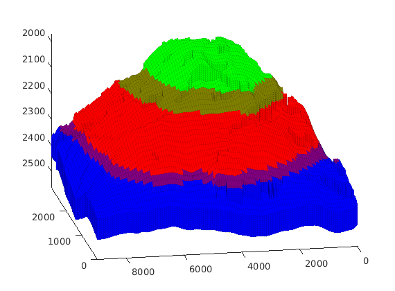
Run the interactive diagnostics¶

We setup the interactive plot and print the help page to show functionality.

help interactiveDiagnostics
clf;
interactiveDiagnostics(G, rock, W, 'state', state);
view(-100, 25)
axis tight

Launch an interactive diagnostics session

  SYNOPSIS:
    interactiveDiagnostics(G, rock, W);
    interactiveDiagnostics(G, rock, W, 'state', state)
    interactiveDiagnostics(G, rock, W, dataset, 'state', state)

  DESCRIPTION:
...

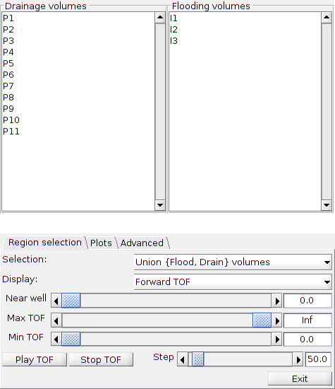
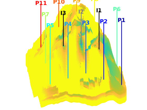
Copyright notice¶

<html>
% <p><font size="-1

Well-Pair Diagnostics for 3D Subset of SPE10¶

Generated from diagnostWellPairs.m

In this example, we show how one can use static tracer partition to visualize drainage and flooded volumes and compute well-pair diagnostics such as volumes, well-allocation factors, etc. We also show how to subdivide wells into multiple segments and use this to study the flow patterns in more detail.

mrstModule add diagnostics spe10 incomp coarsegrid
close all

Set up problem¶

As our example, we consider a subsample of Model 2 from the 10th SPE Comparative Solution Project, but with a new well pattern that has two injectors in the center of the reservoir.

% Grid
cartDims = [  60,  220,  20];
physDims = [1200, 2200, 2*cartDims(end)] .* ft();   % ft -> m
G  = cartGrid(cartDims, physDims);
G  = computeGeometry(G);

% Rock
rock = getSPE10rock(1:cartDims(end));
rock.poro = max(rock.poro, 1e-4);

% Wells
W = [];
wname    = {'P1', 'P2', 'P3', 'P4', 'I1', 'I2'};
wtype    = {'bhp', 'bhp', 'bhp', 'bhp', 'bhp', 'bhp'};
wtarget  = [200,   200,   200,   200,   500,   500  ] .* barsa();
wrad     = [0.125, 0.125, 0.125, 0.125, 0.125, 0.125] .* meter;
wloc     = [  1,   60,     1,   60,  20, 40;
              1,    1,   220,  220, 130, 90];
for w = 1 : numel(wtype),
   W = verticalWell(W, G, rock, wloc(1,w), wloc(2,w), 1 : cartDims(end), ...
                    'Type', wtype{w}, 'Val', wtarget(w), ...
                    'Radius', wrad(w), 'Name', wname{w}, ...
                    'InnerProduct', 'ip_tpf');
end

% Fluid: single-phase flow
fluid = initSingleFluid('mu', 1*centi*poise, 'rho', 1014*kilogram/meter^3);

Show model setup¶

We start by visualizing the reservoir and well pattern. We add a colorbar with a histogram and fiddle somewhat with the graphics handles to get a nice look of the overall figure

fig1=figure('position',[450 450 750 350]);
plotCellData(G,rock.poro, 'EdgeColor','k','EdgeAlpha',.05);
plotWell(G,W,'height',2,'FontSize',14); axis tight;
set(gca,'dataaspect',[1 1 0.06]), view(-60,15); axis off

[hc,hh]=colorbarHist(rock.poro,[.0 .45],'South', 80);
pos=get(hc,'Position'); set(hc,'Position',pos - [-.03 0 .25 .02],'FontSize',12);
pos=get(hh,'Position'); set(hh,'Position',pos - [-.03 0.02 .25 0.03]);
set(gca,'Position',[.13 .17 .775 .785])

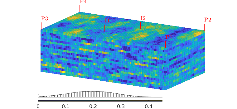
Compute flow solution and diagnostic quantities¶

As usual, we only solve a single-phase flow problem to get the flow field needed for the diagnostics

rS = initState(G, W, 0);
T  = computeTrans(G, rock);
rS = incompTPFA(rS, G, T, fluid, 'wells', W);
D = computeTOFandTracer(rS, G, rock, 'wells', W);

Sweep volumes for I1 and I2¶

We start by showing the sweep volumes for the two injectors. Here, we observe three regions and not the two we expected. The third, and very small, region corresponds to a section of the reservoir that is almost impermeable and hence will not be swept by any of the injetors.

clf(fig1);
plotCellData(G,D.ipart,'EdgeColor','k','EdgeAlpha',.05);
plotWell(G,W,'height',2,'FontSize',14); axis tight; title('Flooded volumes');
set(gca,'dataaspect',[1 1 0.06]), view(-60,15); axis off

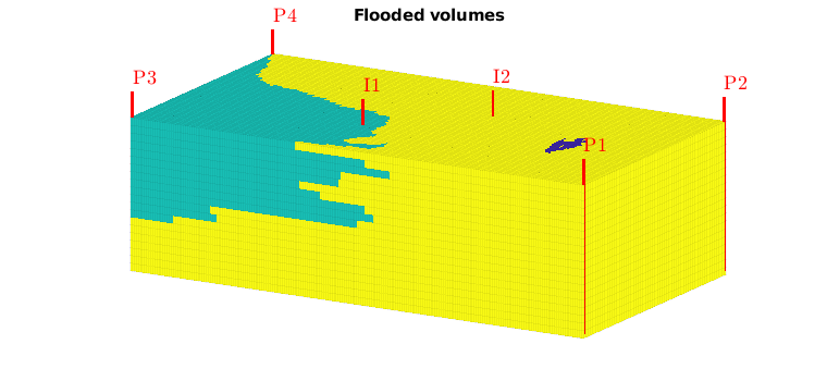
Drainage volumes for P2 to P4¶

Next, we show the drainage volumes for the producers. To be able to look inside the model, we exclude the drainage region for P1, which is closest to the view point.

clf(fig1);
Gbb = cartGrid([1 1 1]);
Gbb.nodes.coords = bsxfun(@mtimes,Gbb.nodes.coords,max(G.nodes.coords));
plotCellData(G,D.ppart,D.ppart>1,'EdgeColor','k','EdgeAlpha',.05);
plotGrid(Gbb,'FaceColor','none');
plotWell(G,W,'height',2,'FontSize',14); axis tight; title('Drainage volumes');
set(gca,'dataaspect',[1 1 0.06]), view(-60,15); axis off

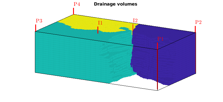
Show refined partition¶

When using a majority vote to determine drainage and sweep regions, we disregard the fact that there are regions that are influenced by more than one tracer. In this visualization, we will blend in a gray color to signify that some regions are influenced by more than one tracer

clf(fig1),
plotTracerBlend(G, D.ppart, max(D.ptracer, [], 2), 'EdgeColor','k','EdgeAlpha',.05)
plotWell(G,W,'height',2,'FontSize',14); axis tight;
set(gca,'dataaspect',[1 1 0.06]), view(-60,15); axis off

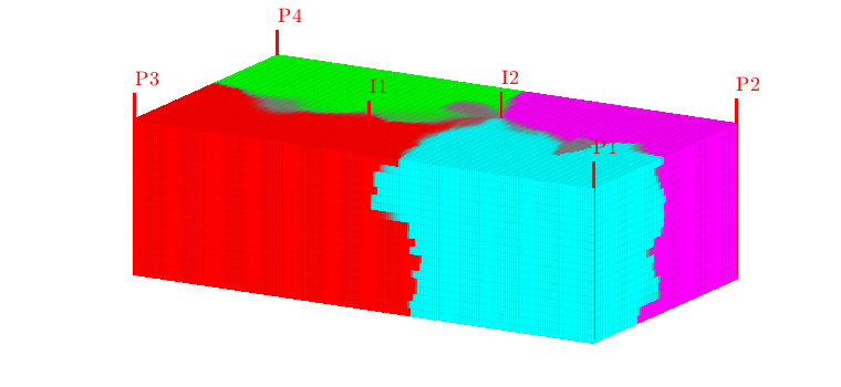
Well pairs¶

Having established the injection and tracer partitions, we can identify well pairs and compute the pore volumes of the regions that can be associated with each well pair.

fig2=figure;
WP = computeWellPairs(rS, G, rock, W, D);
pie(WP.vols, ones(size(WP.vols)));
legend(WP.pairs,'location','Best');

figure(fig1); clf
p = compressPartition(D.ipart + D.ppart*max(D.ipart))-1;
plotCellData(G,p,p>0,'EdgeColor','k','EdgeAlpha',.05);
plotWell(G,W,'height',2,'FontSize',14); axis tight;
set(gca,'dataaspect',[1 1 0.06]), view(-60,15); axis off

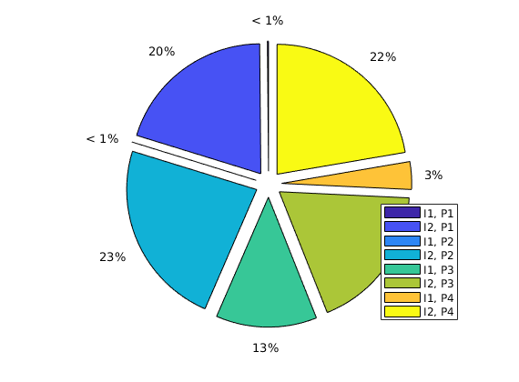
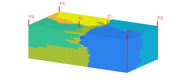
Allocation factors for well pairs¶

We show a bar plot of well allocation factors for each completion of the wells as a function of the depth of the completion. The allocation factor is defined as the normalized, cummulative flux in/out of a well from bottom and up. To investigate how the volumetric connections affect the flow in and out of wells, we can look at well-allocation factors, which are defined as the cumulative flux in/out of a well from toe to heel (here: bottom to top perforation). First, we compute the flux allocation manually for the two injectors

figure(fig1); clf
for i=1:numel(D.inj)
   subplot(1,numel(D.inj),i);
   alloc = cumsum(flipud(WP.inj(i).alloc),1);
   barh(flipud(WP.inj(i).z), alloc,'stacked'); axis tight
   lh=legend(W(D.prod).name,'Location','SouthEast');
   set(gca,'YDir','reverse');   title(W(D.inj(i)).name);
end

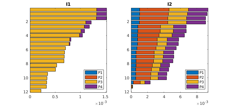
Then we use a library function to compute and visualize the well-allocation factors for all the wells in the model

figure; set(gcf,'Position',[10 70 600 760]);
plotWellAllocationPanel(D, WP);

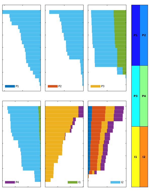
Look at individual completions¶

To look more closely at the performance of the different completions along the well path, we can divide the completion intervals into bins and assign a corresponding set of pseudo wells for which we recompute flow diagnostics. As an example, we split the completions of I1 into three bins and the completions of I2 into four bins.

[rSp,Wp] = expandWellCompletions(rS,W,[5, 3; 6, 4]);
Dp = computeTOFandTracer(rSp, G, rock, 'wells', Wp);

Injector I1¶

figure(fig1); clf
plotCellData(G, Dp.ipart,(Dp.ipart>0) & (Dp.ipart<4), 'EdgeColor','k','EdgeAlpha',.05);
plotWell(G,W,'height',2,'FontSize',14); axis tight;
plotGrid(Gbb,'FaceColor','none');
set(gca,'dataaspect',[1 1 0.06]), view(-60,15); axis off

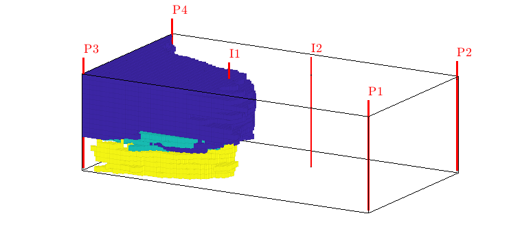
Injector I2¶

figure(fig1); clf
plotCellData(G, Dp.ipart,(Dp.ipart>3) & (Dp.ipart<8), 'EdgeColor','k','EdgeAlpha',.05);
plotWell(G,W,'height',2,'FontSize',14); axis tight;
plotGrid(Gbb,'FaceColor','none');
set(gca,'dataaspect',[1 1 0.06]), view(120,15); axis off

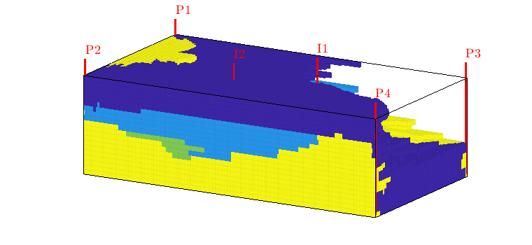
We end the example by computing the fraction of the sweep region for I2 that can be attributed to the different well segments. To this end, we first recompute well-pair regions for all well segments and then use accumarray to sum all well pairs that involve segments from I2.

figure(fig2); clf
WPp = computeWellPairs(rSp, G, rock, Wp, Dp);
avols = accumarray(WPp.pairIx(:,1),WPp.vols);
h = pie(avols(4:end)); set(h(2:2:end),'FontSize',16);

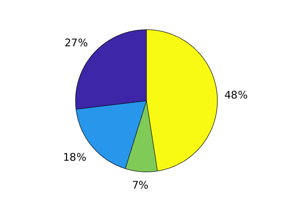
Copyright notice¶

<html>
% <p><font size="-1

Diagnostics GUI using MRST simulation output¶

Generated from diagnosticsPostProcessorWithMRST.m

This example shows how to use the diagnostics post processing GUI and visualise results from MRST simulation output. First we run the Egg model in MRST using the packSimulationProblem setup. Then we load the results into the GUI which calculates the diagnostics and displays them interactively. See also PostProcessDiagnosticsECLIPSE.m

Load relevant modules¶

mrstModule add ad-blackoil ad-core deckformat mrst-gui ad-props diagnostics

Get Eclipse deck for EGG¶

Here we perform simulations on a single realization of the EGG model

deck = getDeckEGG('realization',1);
gravity reset on

Setup model, schedule and initial state¶

We get all necessary parameters from the Eclipse deck

G = initEclipseGrid(deck);
[state0, model, schedule, nonlinear] = initEclipseProblemAD(deck, 'G', G);

Define/pack simulation problem¶

problem = packSimulationProblem(state0, model, schedule, 'egg_model_FlowDiagnostics');

Simulate problem¶

This may take some time to simulate, however if the simulation has been completed already a new call to simulatePackedProblem will recognise that the simulation is complete and will do nothing. If the simulation is aborted, a new call to simulatePackedProblem will continue the simulation. To clear previous results and rerun a simulation use: clearPackedSimulatorOutput(problem);

simulatePackedProblem(problem);

states/wellSols are accessed through handles¶

[ws, states, reports] = getPackedSimulatorOutput(problem);

Run PostProcessDiagnostics¶

PostProcessDiagnosticsMRST takes as input a packed problem, packed using the packSimulationProblem function. The simulation must have been run already to get the flow field at each timestep. Diagnostics are calculated and displayed interactively.

PostProcessDiagnosticsMRST(problem);

Copyright notice¶

<html>
% <p><font size="-1

diagnostics: Flow diagnostics functionality¶

Examples¶

Ranking of different realizations of the same model¶

We first solve the base case using a pressure solver¶

Go through the different cases and store the diagnostics output¶

Plot the different F-Phi diagrams¶

Iterate over all¶

Plot the producer tracer concentrations¶

Plot injector tracers¶

Flow Pattern and Dynamic Heterogeneity for 2D Five-Spot Problem¶

Set up and solve flow problem¶

Compute and display time-of-flight and tracer partitioning¶

Compute and display flow-capacity/storage-capacity diagram¶

Compute the Lorenz coefficient¶

Compute and display sweep efficiency versus dimensionless time¶

Copyright notice¶

Introduction to Flow Diagnostics¶

Set up and solve flow problem¶

Compute basic quantities¶

Forward time-of-flight¶

Backward time-of-flight¶

Residence time¶

Tracer from I1¶

Flooded regions¶

Tracer from P2¶

Drainage regions¶

Well regions: I1<->P1, I2<->P3¶

Compute time-of-flights inside each well region¶

F-Phi diagram¶

Lorenz coefficient¶

Sweep effciency diagram¶

Copyright notice¶

Optimizing Well Placement and Rates¶

Parameters that determine the setup¶

Set up reservoir and fluid properties¶

Set up wells¶

Plot the initial setup¶

Set up objective functions and optimize¶

Plot well paths¶

Plot total travel time for both base and optimized case¶

Plot the storage / flow capacity diagrams¶

Run two-phase simulation to validate the results¶

Plot the recovery at the half-way point¶

Plot both problems in the same plot¶

Copyright notice¶

Well Optimization using Adjoints and Flow Diagnostics¶

Setup model¶

Define objective function and plot domain¶

Optimize well rates¶

Plot the time of flight of the initial and the best well rates¶

Plot sweep and flow capacity diagrams¶

Copyright notice¶

Illustrate use of flow diagnostics to verify upscaling¶

Make model¶

Compute flow on the fine-scale model¶

Flow diagnostics on fine-scale model¶

Coarse-scale solution¶

Flow diagnostics on the upscaled model¶

Display bar charts of flow-allocation factors¶

Display the partition¶

Copyright notice¶

Interactive diagnostics on the SAIGUP dataset¶

Set up grid and rock¶

Set up wells¶

Set up a reservoir state¶

Run the interactive diagnostics¶

Copyright notice¶

Well-Pair Diagnostics for 3D Subset of SPE10¶

Set up problem¶

Show model setup¶

Compute flow solution and diagnostic quantities¶

Sweep volumes for I1 and I2¶

Drainage volumes for P2 to P4¶

Show refined partition¶

Well pairs¶

Allocation factors for well pairs¶

Look at individual completions¶

Injector I1¶

Injector I2¶

Copyright notice¶

`diagnostics`: Flow diagnostics functionality¶