`wellpaths`: Generation of wells using general curves¶

Functionality for defining wells following curvilinear trajectories. By defining each well trajectory as a series of points, this module can combine multiple trajectories and determine which cells are penetrated by the well path. The trajectories can be interpolated using any of Matlab’s built-in routines (splines, piecewise linear functions, etc).

Contents¶

UTILS

Files: combineWellPaths - Combine multiple simple paths into a full tree findWellPathCells - Convert well path to the intersected cells getWellFromPath - Convert well path to MRST well. makeSingleWellpath - Create well path from points (and optional connectivity and active flag) plotWellPath - Plot a well path refineSpline - Refine a curve to higher resolution using spline interpolation

combineWellPaths(wellpaths)¶

Combine multiple simple paths into a full tree

Synopsis:

wellpath = combineWellPaths({wp1, wp2, wp3});

Description:

Given multiple simple well paths this function assembles a single well tree from the inputs. For this to work we assume that:

The paths are ordered by depth in the tree. This is not the

vertical depth, but rather that a path will always be connected to one of the curves preceding it in the list. - Paths (aside from the first one) always start with a point that also exists in one of the preceding paths. This is used to connect the paths.

Parameters:	wellpaths – Cell array of simple well paths to be assembled together. A simple well path is assumed to contain a single list of points (i.e. it will only represent a line segment).
Returns:	wellpath – Composite wellpath made from the simple wellpaths. The topology will be tree-like in nature.

See also

makeSingleWellpath

findWellPathCells(G, wellpath, varargin)¶

Convert well path to the intersected cells

Synopsis:

cells = findWellPaths(G, wellpath);

Description:

By creating a triangulation and mapping perforations to the closest cells, this routine realizes the continuous well path into discrete cells, making it possible to build simulation wells from it.

Keyword Arguments:
Parameters:	G – The grid structure we want to realize the wells on. wellpath – Well path. See “makeSingleWellpath” for spec.
	interpType – The type of interpolation used to extend the curve between points. Supports the same types as MATLAB builtin interp1. Default: Spline. triangulation – The triangulation (typically from delaunayTriangulation) used to determine proximity in the grid. refinement – Refinement number used to further refine the well curve before computing which cells it intersect. Default: 100.
Returns:	cells – The list of cells the well intersects. segment – Segment indicator for each cell, indicating which wellpath segment produced that specific completion. If multiple choices are possible, the segment which comes first in wellpath.points is used. ptsind – Point indicator, indicating which point in the segment was the closest to a given cell. DT – Triangulation used to produce the results.

getWellFromPath(W0, G, rock, wellpath, varargin)¶

Convert well path to MRST well.

Synopsis:

W = getWellFromPath(W, G, rock, wellpath);

Description:

This routine converts a well path (representing curves and points) into a well (represented by cells and connectivity).

Parameters:	W0 – Well array to be extended with the new well. G – The grid the well is to be placed in. rock – Rock structure which defines permeability and porosity. wellpath – Well path as procued by makeSingleWellPath or combineWellPaths. OPTIONAL PARAMETERS: This function calls addWell. Any keyword arguments are passed onto addWell.
Returns:	W – Updated wells

Note

Currently no special effort is made to ensure correct well indices for the well.

See also

plotWellPath, getWellFromPath

plotWellPath(wellpaths, varargin)¶

Plot a well path

Synopsis:

plotWellPath(wellpath)
h = plotWellPath(wellpath, 'color', 'r')

Description:

Plots a given well path, using colors and showing control points along the curve.

Keyword Arguments:
Parameters:	wellpath – Well path to be plotted. See makeSingleWellpath.
	interpType – Interpolation type used. Same possible values as for MATLAB builtin interp1. Default: Spline. LineWidth – Line width of curve used to draw wellpath segments. MarkerColor – Used to colorize the control points. Color – Color of the line segments themselves. Refinement – The path is refined using interpolation to produce nice curves. Entering a positive number here will refine the curve by a number of points. Interpreted as a multiplicative factor.
Returns:	h – Two-column array of handles. The first column contains handles for the line segments and the second for the control point markers.

refineSpline(points, n_refine, interpType)¶

Refine a curve to higher resolution using spline interpolation

Synopsis:

pts = refineSpline(points, 10, 'spline');
pts = refineSpline(points, 5);

Description:

Refine a given curve given as a array of points into

Parameters:

points – A npts x dim array of points giving the curve to be refined. Implicitly assumed to be ordered.
n_refine – The refinement factor. If the original entries in points contained n points, the output will have n_refine*n total points.
interpType – Type of interpolation. Supports the same values as the fourth argument to MATLABs interp1 function. If omitted, it defaults to ‘spline’.

Returns:

pts – Refined points.
v – Parametrization of the new points. Continuous values from 1 to npts indicating how far along interpolated values are on the original trajectory.

Examples¶

Define a model¶

Generated from wellTrajectoryExample.m

mrstModule add ad-core ad-blackoil diagnostics wellpaths
km = kilo*meter;
pdims = [5, 4, 0.01]'*km;

% dims = [50, 40, 10];
dims = [25, 20, 5];

G = cartGrid(dims, pdims);
G = computeGeometry(G);

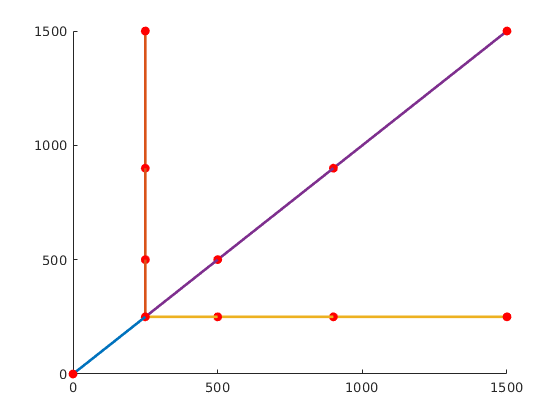
Define a forked well¶

We define four curves, with some common points to combine them into a single well path.

p1 = [0.25, 0.5, 0.9, 1.5]'*km;

n = numel(p1);

z = [.25, 0.5, 0.75, .80]'*pdims(3);

a = [p1(1)*ones(n, 1), p1];
b = [p1,               p1(1)*ones(n, 1)];
c = [p1,               p1];

origin = [0, 0, 0; a(1, :), z(1)];

% First foru well paths.
wellpath0 = makeSingleWellpath(origin);
wellpath1 = makeSingleWellpath([a, z]);
wellpath2 = makeSingleWellpath([b, z]);
wellpath3 = makeSingleWellpath([c, z]);
% Combine into single well path
wellpath_fork = combineWellPaths({wellpath0, wellpath1, wellpath2, wellpath3});

% Plotting
clf;
plotWellPath(wellpath_fork);

Make a comb-like well¶

x = [3, 3.5, 4, 4.5]'*km;
y = [3.5, 3, 2.5, 2]'*km;

y0 = [3.75*km; y];
x0 = x(end)*ones(numel(y)+1, 1);

dz = 1/numel(y);
z0 = (0:dz:1)'*pdims(3);

wp0 = [x0, y0, z0];

n0 = numel(x0);

wellpaths = cell(5, 1);

wellpaths{1} = makeSingleWellpath(wp0);

for i = 1:4
    n = numel(x);
    wp = [x, repmat(y(i), n, 1), repmat(z0(i+1), n, 1)];
    wellpaths{i+1} = makeSingleWellpath(wp(end:-1:1, :));
end

wellpath_comb = combineWellPaths(wellpaths);

Determine the cells¶

[cells_fork, segInd_fork, ~, ~, DT] = findWellPathCells(G, wellpath_fork);
[cells_comb, segInd_comb] = findWellPathCells(G, wellpath_comb, 'triangulation', DT);

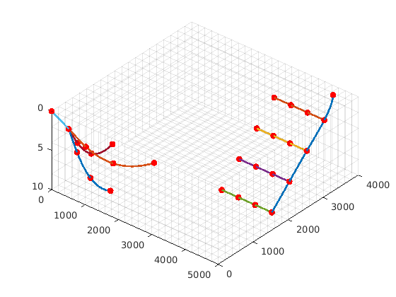
Plot the well trajectories¶

clf;
plotWellPath(wellpath_comb);
plotWellPath(wellpath_fork);

plotGrid(G, 'facec', 'none', 'edgea', .1)
view(40, 56)

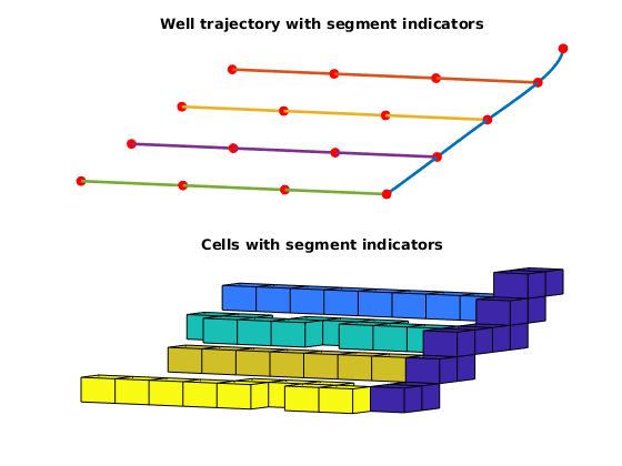
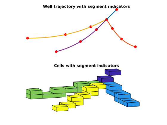
Plot wells individually + realized cell perforations¶

close all
for i = 1:2
    if i == 1
        wp = wellpath_comb;
        si = segInd_comb;
        c = cells_comb;
        v = [30, 12];
    else
        wp = wellpath_fork;
        si = segInd_fork;
        c = cells_fork;
        v = [160, 40];
    end

    figure;
    subplot(2, 1, 1)
    plotWellPath(wp);
    view(v);
    title('Well trajectory with segment indicators')
    axis tight off

    subplot(2, 1, 2)
    plotCellData(G, si, c)
    view(v);
    title('Cells with segment indicators')
    axis tight off
end

Set up actual simulation wells from the well paths¶

Initial reservoir state

initSat = [.1, .9];
state = initResSol(G, 200*barsa, initSat);
% Rock
rock = makeRock(G, 300*milli*darcy, 0.5);

time = 10*year;
rate = .25*sum(poreVolume(G, rock))/time;

segInd = cell(2, 1);
W = [];
[W, segInd{1}]  = getWellFromPath(W, G, rock, wellpath_fork, ...
    'comp_i', [1 0], 'val', 300*barsa, 'type', 'bhp', 'sign', -1, 'Name', 'Producer');
[W, segInd{2}] = getWellFromPath(W, G, rock, wellpath_comb,...
    'comp_i', [1 0], 'val', rate, 'type', 'rate', 'sign', 1, 'Name', 'Injector');

Set up simulation model¶

mrstModule add ad-core ad-blackoil ad-props

fluid = initSimpleADIFluid('rho', [1000, 700, 100]*kilogram/meter^3, ...
                           'mu', [1, 10 1]*centi*poise);

model = TwoPhaseOilWaterModel(G, rock, fluid);

model.extraStateOutput = true;
model.extraWellSolOutput = true;

Build a schedule¶

n = 50;
dt = time/n;
timesteps = repmat(dt, n, 1);
schedule = simpleSchedule(timesteps, 'W', W);

[ws, states] = simulateScheduleAD(state, model, schedule);

Solving timestep 01/50:          -> 73 Days
Solving timestep 02/50: 73 Days  -> 146 Days
Solving timestep 03/50: 146 Days -> 219 Days
Solving timestep 04/50: 219 Days -> 292 Days
Solving timestep 05/50: 292 Days -> 1 Year
Solving timestep 06/50: 1 Year   -> 1 Year, 73 Days
Solving timestep 07/50: 1 Year, 73 Days -> 1 Year, 146 Days
Solving timestep 08/50: 1 Year, 146 Days -> 1 Year, 219 Days
...

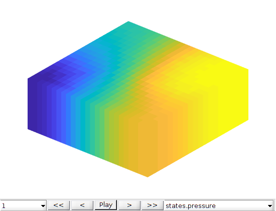
Plot well curves + reservoir properties¶

mrstModule add mrst-gui
figure;
plotToolbar(G, states);
axis tight off
view(40, 56);
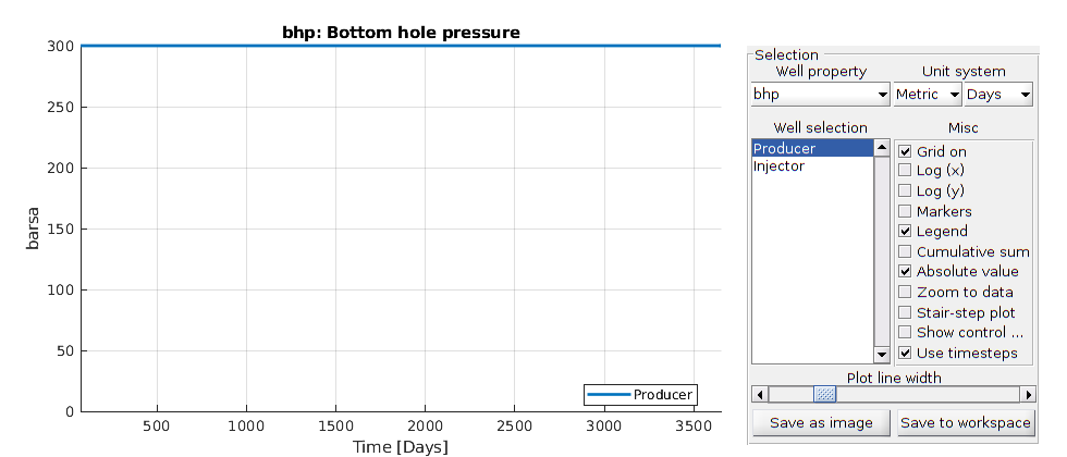
T = cumsum(schedule.step.val);

plotWellSols(ws, T)

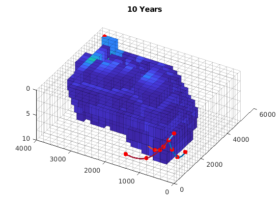
Plot the saturation front¶

close all
plotWellPath(wellpath_comb);
plotWellPath(wellpath_fork);

plotGrid(G, 'facec', 'none', 'edgea', .2);
view(-60, 60);
h = nan;
for i = 1:numel(states)
    if ishandle(h); delete(h); end

    s = states{i}.s(:, 1);
    h = plotCellData(G, s, s > 0.2, 'edgea', .2);
    title(formatTimeRange(T(i)));
    pause(0.25)
end

Apply some flow diagnostics…¶

diagstate = states{end};
[state_split, Wc] = expandWellCompletions(diagstate, W, segInd);
D  = computeTOFandTracer(state_split, G, rock, 'wells', Wc);
WP = computeWellPairs(state_split, G, rock, Wc, D);

Plot results¶

figure; plotToolbar(G, D)
plotWellPath(wellpath_comb);
plotWellPath(wellpath_fork);

wellpaths: Generation of wells using general curves¶

Examples¶

Define a model¶

Define a forked well¶

Make a comb-like well¶

Determine the cells¶

Plot the well trajectories¶

Plot wells individually + realized cell perforations¶

Set up actual simulation wells from the well paths¶

Set up simulation model¶

Build a schedule¶

Plot well curves + reservoir properties¶

Plot the saturation front¶

Apply some flow diagnostics…¶

Plot results¶

`wellpaths`: Generation of wells using general curves¶