`vemmech`: Mechanics for general grids using the virtual element method¶

Geomechanics with the Virtual Element Method

The virtual element method (VEM) is a generalization of the finite element method to very general pologonal and polyhedral grids. The method takes inspiration from mimetic methods (see the ‘mimetic’ module) and is designed to fulfill the patch test, i.e., reproduce exact solutions for displacements that vary linearly in space (strain solutions).

The module contains a preliminary implementation of VEM for linear elasticity and poro eleasticity, and includes several examples with grids combining tetrahedal, hexahedral, and general polygonal elements. The tutorial examples do not offer much explaination or discussion of results, and the computational routines are not yet fully documented. Despite this, we have decided to publish the module ahead of time after several people have asked us to do so.

Contents¶

UTILS

Files: addFluidContribMechVEM - SYNOPSIS: C2D - Compute the matrix of normalized strain energies (D) from the elasticity calStressEigsVEM - calculate eigen values of stress tensor and the basis calculateQC - SYNOPSIS: calculateQF - SYNOPSIS: calculateStressVEM - Undocumented Utility Function complex3DGrid - SYNOPSIS: Enu2C - For each cell, construct the 3x3 (in 2D) or 6x6 (in 3D) matrix representing ENu2LMu_3D - SYNOPSIS: exploreSquareGrid - Explore the different types of grids that can be set up using the function squareGrid lincompTPFA - Solve weakly compressible flow problem (fluxes/pressures) using TPFA method. linearDisplacement - SYNOPSIS: squareGrid - SYNOPSIS: squareLayersTest - SYNOPSIS: squareTest - Different test cases for linear elasticity on square domains VEM2D_div - Discrete div operator for the virtual element method in 2D VEM3D_div - Discrete div operator for the virtual element method in 3D VEM_div - Discrete div operator for the virtual element method

exploreSquareGrid¶: Explore the different types of grids that can be set up using the function squareGrid

C2D(C, G, varargin)¶

Compute the matrix of normalized strain energies (D) from the elasticity tensor (C) associated with grid (G).

convert Stiffness tensor from Voigt notation to plain notations (no factors are applied to the off-diagonal coefficients of the strain tensor). The latter is used in our formulation of VEM. The resulting tensor D is such that, for S in plain notation, we have: S’DS = energy.

ENu2LMu_3D(E, nu)¶

Synopsis:

function [lambda, mu] = ENu2LMu_3D(E, nu)

DESCRIPTION: Compute the Lamé parameters lambda and mu in the 2D case from the Young’s modulus E and Poisson’s ratio Nu. In the orthogonal direction (with respect to the 2D plane), it is assumed zero displacement. In particular, it implies that Nu = 0.5 corresponds as in the 3D case to an incompressible material. An other assumption, which is not used here, could be that there is no stress in the orthogonal direction.

Parameters:	E – Young’s modulus nu – Poisson’s ratio
Returns:	lambda – First Lamé coefficient mu – Second Lamé coefficient

EXAMPLE:

SEE ALSO:

Enu2C(E, nu, G)¶

For each cell, construct the 3x3 (in 2D) or 6x6 (in 3D) matrix representing the elasticity tensor.

Synopsis:

function C = Enu2C(E, nu, G)

DESCRIPTION:

In 3D, the matrix of the elasticity tensor for a given cell is written:

1-nu  nu    nu    0          0          0         |
nu    1-nu  nu    0          0          0         |
nu    nu    1-nu  0          0          0         |            E
0     0     0     (1-2nu)/2  0          0         |  x  ————–
0     0     0     0          (1-2nu)/2  0         |     (1+nu) (1-2nu)
0     0     0     0          0          (1-2nu)/2 |

In 3D, the inverse of the elasticity tensor is given by

[ [ 1 / E, -(nu / E), -(nu / E), 0, 0, 0 ]: [ -(nu / E), 1 / E, -(nu / E), 0, 0, 0 ] [ -(nu / E), -(nu / E), 1 / E, 0, 0, 0 ] [ 0, 0, 0, 2*(nu + 1) / E, 0, 0 ] [ 0, 0, 0, 0, 2*(nu + 1) / E, 0 ] [ 0, 0, 0, 0, 0, 2*(nu + 1) / E ] ]

In 2D, the inverse is given

[ [ 1 - nu, -nu, 0 ] 1 + nu: [ -nu, 1 - nu, 0 ] x ————– [ 0, 0, 2 ] ] E

The factors 2 in the expressions of the inverse above are due to Voigts notations, see https://en.wikipedia.org/wiki/Voigt_notation

invCi = C^{-1}*(Identity tensor)

Parameters:	E – Young’s modulus (one entry per cell) nu – Poisson ratio (one entry per cell) G – Grid
Returns:	C – (k,n) matrix, where k=3^2 (2D) or k=6^2 (3D), and n is the number of cells. Each row thus represents the entries of the elasticity tensor for a specific cell.

VEM2D_div(G, varargin)¶

Discrete div operator for the virtual element method in 2D

Synopsis:

function [div] = VEM2D_div(G)

DESCRIPTION: Computes a discrete div operator in 2D. This discrete div operator is a mapping from node-valued displacement vector to cell-valued 2D vector. Node-valued displacement vectors correspond to the degrees of freedom that determine for each cell a displacement function over the cell via the virtual basis function. The discrete div operator that is assembled here computes the L^2 projection, cell-wise, of this displacement function. For more detail, see paper [Andersen et al: http://arxiv.org/abs/1606.09508v1].

Keyword Arguments:
Parameters:	G – Grid structure
	‘extraFaceDof’ – This option has to be set to get a stable divergence operator when extra degrees of freedom have been introduced on the edges to avoid numerical locking.
Returns:	div – matrix corresponding to the discrete div operator.

EXAMPLE:

SEE ALSO:

VEM3D_div(G)¶

Discrete div operator for the virtual element method in 3D

Synopsis:

function [div] = VEM3D_div(G)

DESCRIPTION: Computes a discrete div operator in 3D. This discrete div operator is a mapping from node-valued displacement vector to cell-valued 2D vector. Node-valued displacement vectors correspond to the degrees of freedom that determine for each cell a displacement function over the cell via the virtual basis function. The discrete div operator that is assembled here computes the L^2 projection, cell-wise, of this displacement function. For more detail, see paper [Andersen et al: http://arxiv.org/abs/1606.09508v1].

Parameters:	G – Grid structure
Returns:	div – matrix corresponding to the discrete div operator.

EXAMPLE:

SEE ALSO:

VEM_div(G)¶

Discrete div operator for the virtual element method

Synopsis:

function [div] = VEM_div(G)

DESCRIPTION: Computes a discrete div operator. This discrete div operator is a mapping from node-valued displacement vector to cell-valued vector. Node-valued displacement vectors correspond to the degrees of freedom that determine for each cell a displacement function over the cell via the virtual basis function. The discrete div operator that is assembled here computes the L^2 projection, cell-wise, of this displacement function. For more detail, see paper [Andersen et al: http://arxiv.org/abs/1606.09508v1].

Parameters:	G – Grid struture
Returns:	div – matrix corresponding to the discrete div operator.

EXAMPLE:

SEE ALSO:

addFluidContribMechVEM(G, bc, rock, isdirdofs)¶

Synopsis:

function fbc = addFluidContribMechVEM(G, bc, rock, isdirdofs)

DESCRIPTION: Setup the force boundary condition for the mechanics corresponding to the fluid boundary condition.

Parameters:	G – Grid structure bc – Fluid boundary conditions. rock – Rock structure isdirdofs – Degrees of freedom where in fact Dirichlet boundary conditions are imposed
Returns:	fbc – Force load for the mechanical system.

EXAMPLE:

SEE ALSO:

calStressEigsVEM(G, stress, varargin)¶

calculate eigen values of stress tensor and the basis

transform to traditional voits notation (for stress this has no factors)

calculateQC(G)¶

Synopsis:

function [qc, qf, qcvol] = calculateQC(G)

DESCRIPTION: Calculate elementary integrals that are used to assemble the stiffness matrix for the 3D case. The precise definitions can be found in [Gain et al: doi:10.1016/j.cma.2014.05.005].

Parameters:	G – Grid structure
Returns:	qc – Elementary assembly integrals : One (3D) vector value in each cell, see (74) in [Gain et al]. qf – Elementary assembly integrals : One scalar value for each face for each node, corresponds to (98) in [Gain et al]. qcvol – Elementary assembly integrals : One scalar value for each node in each cells, gives weights to compute the L^2 projections, see VEM_linElast.m

EXAMPLE:

SEE ALSO:

calculateQF(G)¶

Synopsis:

function [qf, qf_vol] = calculateQF(G)

DESCRIPTION: Calculate elementary integrals that are used to assemble the stiffness matrix for the 2D case.

Parameters:

G – Grid structure

Returns:

qf – Elementary assembly integrals : One (2D) vector value in each cell, which corresponds to the two components of the integral of the basis function in each coordinate over the faces (see (74) in [Gain et al: doi:10.1016/j.cma.2014.05.005], then faces there correspond to edges here).
qf_vol – Elementary assembly integrals : one scalar value for each node, wich corresponds to the weights that are used to compute th L^2 projection, see VEM_linElast.m

EXAMPLE:

SEE ALSO:

calculateStressVEM(G, uu, op, varargin)¶: Undocumented Utility Function

complex3DGrid(opt, grid_case)¶

Synopsis:

function [G, G_org] = complex3DGrid(opt, grid_case)

DESCRIPTION:

Parameters:

opt –
Parameter structure with fields L - Physical dimension (‘box’ and ‘grdecl’ case) cartDims - Cartesian dimension (‘box’ and ‘grdecl’ case) disturb - disturbance parameter for the grid (‘box’ case) triangulate - If true, the horizontal faces are triangulated. vertical - Only relevant for Norne grid (straightens up

the pillars, see paper [Andersen et al: http://arxiv.org/abs/1606.09508v1])

gtol - Grid tolerance parameter (used when calling

processGRDECL, see documentation there)

ref - Refinement parameter, only used for Norne grid
grid_case – 3D Grid cases that are set up here. ‘box’ - grid set up using squareGrid function ‘grdecl’ - grid set up using Eclipse format ‘sbed’ - run dataset_bedmodel2() to get a full description ‘Norne’ - run dataset_norne() to get a full description

Returns:

G – Grid that has been created
G_org – Original grid without refinement (only ‘Norne’ case)

Example:

G=complex3DGrid(struct('vertical',true,'triangulate',false,'ref',1,'gtol',1e-3),'norne');clf,plotGrid(G),view(3)
G=complex3DGrid(struct('triangulate',false,'gtol',1e-3),'sbed');clf,plotGrid(G),view(3)
G=complex3DGrid(struct('triangulate',true,'gtol',1e-3),'sbed');clf,plotGrid(G),view(3)
G=complex3DGrid(struct('triangulate',false,'gtol',1e-3),'sbed');clf,plotGrid(flipGrid(G)),view(3)
G=complex3DGrid(struct('cartDims',[3,3,3],'L',[3 3 3],'disturb',0.04,'triangulate',false),'box');clf,plotGrid(G),view(3)
G=complex3DGrid([],'grdecl'); clf, plotGrid(G), view(3)

lincompTPFA(dt, state, G, T, pv, fluid, rock, varargin)¶

Solve weakly compressible flow problem (fluxes/pressures) using TPFA method.

Synopsis:

state = lincompTPFA(state, G, T, fluid)
state = lincompTPFA(state, G, T, fluid, 'pn1', pv1, ...)

Description:

This function assembles and solves a (block) system of linear equations defining interface fluxes and cell pressures at the next time step in a sequential splitting scheme for the reservoir simulation problem defined by Darcy’s law and a given set of external influences (wells, sources, and boundary conditions).

This function uses a two-point flux approximation (TPFA) method with minimal memory consumption within the constraints of operating on a fully unstructured polyhedral grid structure.

Parameters:

state – Reservoir and well solution structure either properly initialized from functions ‘initResSol’ and ‘initWellSol’ respectively, or the results from a previous call to function ‘lincompTPFA’ and, possibly, a transport solver such as function ‘implicitTransport’.
T (G,) – Grid and half-transmissibilities as computed by the function ‘computeTrans’.
fluid – Fluid object as defined by function ‘initSimpleFluid’.

Keyword Arguments:

wells – Well structure as defined by function ‘addWell’. May be empty (i.e., W = struct([])) which is interpreted as a model without any wells.
bc – Boundary condition structure as defined by function ‘addBC’. This structure accounts for all external boundary conditions to the reservoir flow. May be empty (i.e., bc = struct([])) which is interpreted as all external no-flow (homogeneous Neumann) conditions.
src – Explicit source contributions as defined by function ‘addSource’. May be empty (i.e., src = struct([])) which is interpreted as a reservoir model without explicit sources.
LinSolve – Handle to linear system solver software to which the fully assembled system of linear equations will be passed. Assumed to support the syntax

x = LinSolve(A, b)

in order to solve a system Ax=b of linear equations. Default value: LinSolve = @mldivide (backslash).
MatrixOutput – Whether or not to return the final system matrix ‘A’ to the caller of function ‘lincompTPFA’. Logical. Default value: MatrixOutput = FALSE.
verbose – Enable output. Default value dependent upon global verbose settings of function ‘mrstVerbose’.
condition_number – Display estimated condition number of linear system.

Returns:

state – Update reservoir and well solution structure with new values for the fields:

pressure – Pressure values for all cells in the

discretised reservoir model, ‘G’.

facePressure –

Pressure values for all interfaces in the discretised reservoir model, ‘G’.

flux – Flux across global interfaces corresponding to

the rows of ‘G.faces.neighbors’.

A – System matrix. Only returned if specifically

requested by setting option ‘MatrixOutput’.

wellSol – Well solution structure array, one element for

each well in the model, with new values for the fields:

flux – Perforation fluxes through all

perforations for corresponding well. The fluxes are interpreted as injection fluxes, meaning positive values correspond to injection into reservoir while negative values mean production/extraction out of reservoir.

pressure – Well bottom-hole pressure.

Note

If there are no external influences, i.e., if all of the structures ‘W’, ‘bc’, and ‘src’ are empty and there are no effects of gravity, then the input values ‘xr’ and ‘xw’ are returned unchanged and a warning is printed in the command window. This warning is printed with message ID

‘lincompTPFA:DrivingForce:Missing’

Example:

G   = computeGeometry(cartGrid([3, 3, 5]));

f   = initSingleFluid('mu' , 1*centi*poise, ...
                      'rho', 1000*kilogram/meter^3);
rock.perm = rand(G.cells.num, 1)*darcy()/100;

bc  = pside([], G, 'LEFT', 2*barsa);
src = addSource([], 1, 1);
W   = verticalWell([], G, rock, 1, G.cartDims(2), []   , ...
                   'Type', 'rate', 'Val', 1*meter^3/day, ...
                   'InnerProduct', 'ip_tpf');
W   = verticalWell(W, G, rock, G.cartDims(1), G.cartDims(2), [], ...
                   'Type', 'bhp', 'Val', 1*barsa, ...
                   'InnerProduct', 'ip_tpf');

T   = computeTrans(G, rock);

state         = initResSol (G, 10);
state.wellSol = initWellSol(G, 10);

state = lincompTPFA(state, G, T, f, 'bc', bc, 'src', src, ...
                   'wells', W, 'MatrixOutput', true);

plotCellData(G, state.pressure)

SEE ALSO:

squareGrid(cartDims, L, varargin)¶

Synopsis:

G = squareGrid(cartDims, L, varargin)

DESCRIPTON: Make square with different irregular grid types starting from cartesian.

run script exploreSquareGrid.m to see the different possibilities

Keyword Arguments:
Parameters:	cartDims – Cartesian dimensions L – Physical lengths
	grid_type – Possible types are ‘cartgrid’ ‘triangle’ ‘pebi’ ‘boxes[1-4]’ ‘mixed[1-4]’. Run the scripts given in the comments below to see how the grid look likes. Only the ‘cartgrid’ type is implemented for 3D. The others apply uniquely for 2D. disturb – The grids can be twisted, essentially to break the Cartesian structure. The parameter disturb determines the amount of twisting that is introduced.
Returns:	G – Grid structure

squareLayersTest(varargin)¶

Synopsis:

function [G, bc, test_cases] = squareLayersTest(varargin)

DESCRIPTION: make test cases for linear elasticity with several layers

Parameters:	varargin –
Returns:	G bc test_cases

squareTest(varargin)¶

Different test cases for linear elasticity on square domains

Synopsis:

function [G, bc, test_cases] = squareTest(varargin)

DESCRIPTION: Set up different test cases to test the linear elasticity code.

Keyword Arguments:

‘L’ – Physical dimension
‘cartDims’ – Cartesian dimension
‘grid_type’ – grid type (see squareGrid function)
‘disturb’ – Disturbance coefficient
‘E’ – Young’s modulus
‘nu’ – Poisson’s ratio
‘make_testcases’ – If true, compute linear displacement test cases.
‘test_name’ – test case name. The alternatives are ‘original_2D_test’ ‘hanging_rod_2D’ ‘weighted_slop_rod_2D_dir’ ‘weighted_slop_rod_2D’ ‘weighted_slop_rod_2D_nobcleftright’ ‘rod_2D_pressure’ ‘rod_2D_pressure_nobcleftright’ ‘rod_2D_point_pressure’ ‘rod_2D_point_pressure_noleftrighbc’ ‘all’

Returns:

G – Grid structure
bc – Boundary conditions
test_cases – Cell structure with the test cases

Contents¶

GRID_UTILS

Files: flipGrid - Flip a grid (z->x, x->y, y->z) padGrdecl - Add padding to corner-point grid so it is embedded in a box verticalGrdecl - Transform GRDECL pillars into vertical pillars

flipGrid(G)¶

Flip a grid (z->x, x->y, y->z)

Synopsis:

function G_new = flipGrid(G);

DESCRIPTION: Flip the grid (z->x, x->y, y->z)

Parameters:	G – Grid structure
Returns:	G_new – Grid structure afte flipping

padGrdecl(grdecl, dirs, box, varargin)¶

Add padding to corner-point grid so it is embedded in a box

Synopsis:

function grdecl_new = padGrdecl(grdecl, dirs, box, varargin)

DESCRIPTION: Adds padding on all the sides of a corner point grid in order to make it a Cartesian box

Keyword Arguments:
Parameters:	grdecl – Grid in eclipse format dirs – Padding directions box – Size of elements in each padding layer
	relative
Returns:	grdecl_new – Grid in eclipse format, with padding.

verticalGrdecl(grdecl, varargin)¶

Transform GRDECL pillars into vertical pillars

Synopsis:

function grdecl = verticalGrdecl(grdecl, varargin)

DESCRIPTION: Straightened up the pillars in a corner point grid, given in Eclipse, and make them vertical

Parameters:

grdecl – Grid structure in Eclipse format

Keyword Arguments:

method – ‘all’ : all pillars are made vertical

‘sides’ : Only the pillare on the sides are made vertical

Returns:

grdecl – Grid structure with vertical pillars in Eclipse format.

EXAMPLE: SEE ALSO:

Contents¶

MODELS

Files: LinearCompressibilityModel -

Contents¶

PLOTTING

Files: plotCellDataDeformed - SYNOPSIS: plotFaceDataDeformed - SYNOPSIS: plotFaces2D - Undocumented Utility Function plotGridDeformed - SYNOPSIS: plotNodeDataDeformed - SYNOPSIS:

plotCellDataDeformed(G, data, u, varargin)¶

Synopsis:

function h = plotCellDataDeformed(G, data, u, varargin)

DESCRIPTION: Plot cell data on a grid which is deformed using a given displacement field.

Parameters:	G – Grid structure data – Data to be plotted u – Displacement field varargin – Optional parameters that are passed further to the function plotCellData
Returns:	h – handle to plot

EXAMPLE:

SEE ALSO:

plotNodeDataDeformed(G, node_data, uu, varargin)¶

Synopsis:

plotNodeDataDeformed(G, node_data, uu, varargin)

DESCRIPTION: Plot node data on a grid which is deformed using a given displacement field.

Parameters:	G – Grid data structure. node_data – node data to be plotted 'pn'/pv – List of other property name/value pairs. OPTIONAL. This list will be passed directly on to function PATCH meaning all properties supported by PATCH are valid.
Returns:	h – Handle to resulting PATCH object. The patch object is added to the current AXES object.

EXAMPLE:

Examples¶

Compaction test case in 2D¶

Generated from compactionTest2D.m

mrstModule add vemmech

Define the fluid and rock parameters and set up the grid.¶

opt = struct('grid_type', 'cartgrid', ...
% see squareGrid
            'disturb'   , 0.0, ...
     % parameter for disturbing grid
            'E'         , 0.3*1e9, ...
 % young's modulus
            'nu'        , 0.4, ...
            'islinear'  , false);       % poisson's ratio

opt.cartDims       = [10 10];
opt.L              = [15*10/10 15];
opt.hanging        = false;
opt.free_top       = true; % If true, the nodes at the top can move freely (no
                           % boundary condition given there)
opt.triangulate    = true; % If true, the horizontal faces are triangulated.
opt.gravity_load   = true; % Use gravity load
opt.top_load       = false;
opt.gtol           = 0.1e-1; % Grid tolerance parameter (used when calling
                             % processGRDECL, see documentation there)
opt.twist          = true;
opt.disturb        = 0.05;
% Different methods are implemented to compute the loading term, see
% paper [Andersen et al: http://arxiv.org/abs/1606.09508v1].
opt.force_method   = 'cell_force'; % 'dual_grad_type'

G = squareGrid(opt.cartDims, opt.L, 'grid_type', opt.grid_type);

if(opt.triangulate)
    face = unique(G.cells.faces(any(bsxfun(@eq, G.cells.faces(:, 2), [3, 4]), 2), 1));
    G = triangulateFaces(G, face);
    G = sortEdges(G);
end

if (opt.twist)
    G = twister(G, opt.disturb);
end

G = createAugmentedGrid(G);
G = computeGeometry(G);

Ev  = repmat(opt.E, G.cells.num, 1);
nuv = repmat(opt.nu, G.cells.num, 1);
C   = Enu2C(Ev, nuv, G);

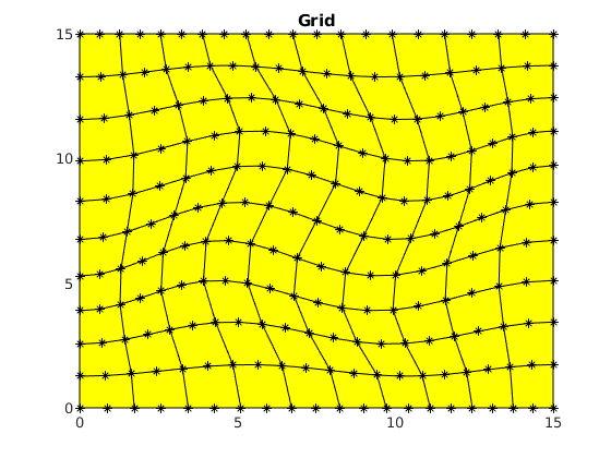
figure()
clf,
plotGrid(G, 'Marker', '*')
title('Grid')

Setup the loads and the boundary conditions¶

% We use the utility function makeCompactionTest
[el_bc, load] = makeCompactionTest(G, opt);

Assemble and solve the system¶

bbsize = 30000-(G.griddim-2)*20000; % block size for the assembly
uu = VEM_linElast(G, C, el_bc, load, ...
                  'blocksize'   , bbsize, ...
                  'force_method', opt.force_method);

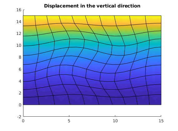
figure(),
clf
plotNodeDataDeformed(G, uu(:, G.griddim), uu);
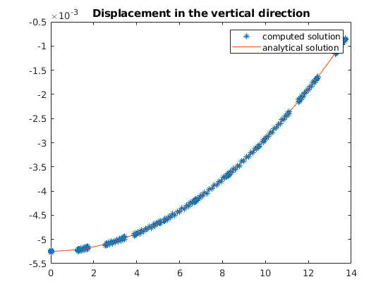
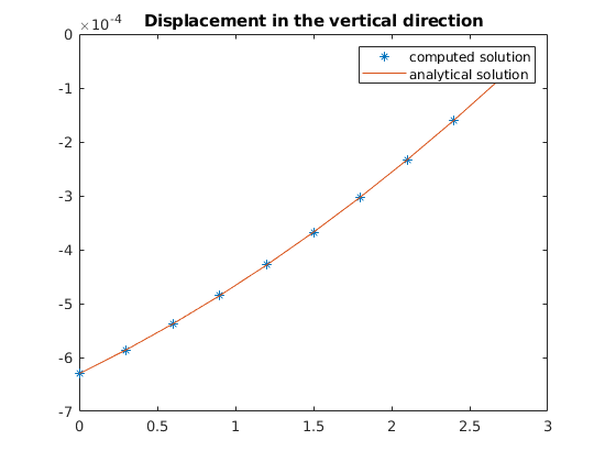
title('Displacement in the vertical direction')

Computation of the analytical solution¶

if(~isempty(el_bc.force_bc))
    ff = abs(el_bc.force_bc.force(1, G.griddim));
else
    ff = 0;
end
start = max(G.faces.centroids(:, G.griddim));
top   = min(G.faces.centroids(:, G.griddim));

fac = 100*300/2;

ana = @(z) ff*(z-start)./(C(1, 1))-double(opt.gravity_load)*fac*((top-start).^2 - (z-top).^2)/C(1, 1);
divana = @(z) (ff./C(1, 1))-double(opt.gravity_load)*fac*(-2*(z-top))/C(1, 1);

Comparison plots¶

z = G.nodes.coords(:, G.griddim);
z(abs(ana(z))<max(abs(ana(z)))*1e-2) = nan;
zl = unique(z);

figure(),
plot(z, uu(:, G.griddim), '*', zl, ana(zl))
title('Displacement in the vertical direction')
legend({'computed solution', 'analytical solution'})

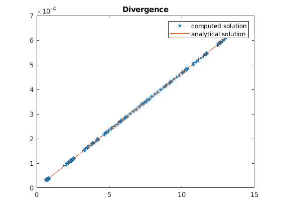
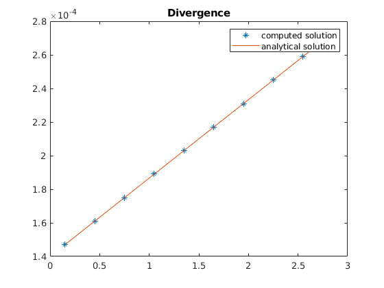
figure()
zc = G.cells.centroids(:, G.griddim);
div = VEM_div(G);
plot(zc, div*reshape(uu', [], 1)./G.cells.volumes, '*', zc, divana(zc));
title('Divergence');
legend({'computed solution', 'analytical solution'})

Compaction test case 3D¶

Generated from compactionTest3D.m

Load required modules¶

mrstModule add vemmech

Define the fluid and rock parameters and set up the grid.¶

opt = struct('grid_type' , 'triangle', ...
             'disturb'   , 0.0, ...
    % parameter for  grid distortion
             'E'         , 0.3*1e9, ...
% Young's modulus
             'nu'        , 0.4, ...
    % Poison's ratio
             'islinear'  , false);
opt.L            = [15 15 3];
opt.islinear     = false; % if true, the boundary condition is a given linear
                          % displacement, see function makeCompactionTest.
% Different methods are implemented to compute the loading term, see
% paper [Andersen et al: http://arxiv.org/abs/1606.09508v1].
opt.force_method = 'dual_grad_type';
opt.hanging      = false; % If true, zero displacement on the vertical sides.
opt.free_top     = true;  % If true, the nodes at the top can move freely (no
                          % boundary condition given there)
opt.triangulate  = false;  % If true, the horizontal faces are triangulated.
opt.vertical     = false; % Only relevant for norne test case (straightens up
                          % the pillars, see paper [Andersen et al: http://arxiv.org/abs/1606.09508v1])
opt.gravity_load = true;  % Use gravity load
opt.top_load     = true;  % Use force applied at the top
opt.gtol         = 0.1e-1; % Grid tolerance parameter (used when calling
                           % processGRDECL, see documentation there)
opt.ref          = 10;     % Refinement parameter, only used for Norne
opt.flipgrid     = false;  % Rotate the grid (z->x, x->y, y->z) (see paper [Andersen et al: http://arxiv.org/abs/1606.09508v1])
if isempty(mfilename)
    % Running example interactively
    grid_case_number = input(['Choose a grid (type corresponding number): box [1], ' ...
                              'sbed [2], Norne [3]\n']);
else
    % Running example as a function
    grid_case_number = 1;
end
switch grid_case_number
  case 1
    grid_case = 'box';
    opt.cartDims     = [[1 1]*3 10]; % set the Cartesian dimension for the box case
  case 2
    grid_case = 'sbed';
  case 3
    grid_case = 'norne';
  otherwise
    error('Choose grid case by typing number between 1 and 3.');
end

G = complex3DGrid(opt, grid_case);

if (opt.flipgrid)
    G = flipGrid(G);
end
G = createAugmentedGrid(G);
G = computeGeometry(G);

Ev     = repmat(opt.E, G.cells.num, 1);
nuv    = repmat(opt.nu, G.cells.num, 1);
C      = Enu2C(Ev, nuv, G);

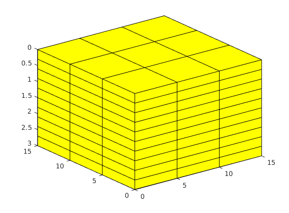
figure()
clf;
plotGrid(G);
view(3);

Setup the loads and the boundary conditions¶

if(strcmp(grid_case,'norne'))
    %only rolling in vertical direction this is need since norne has
    %irregular sides and the code do not have genneral implementation of
    %rolling condition at this point
    [el_bc, load] = makeCompactionTest(G, opt, 'rolling_vertical', true);
else
    [el_bc, load] = makeCompactionTest(G, opt);
end

Assemble and solve the system¶

bbsize = 30000-(G.griddim-2)*20000;
lsolve = @mldivide;
fprintf('Running ...
');
uu = VEM_linElast(G, C, el_bc, load, 'linsolve', lsolve, 'blocksize', bbsize, ...
                  'force_method', opt.force_method);
fprintf('done!\n');

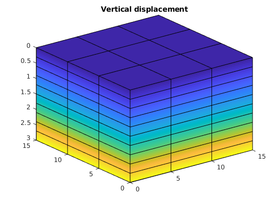
figure();
clf;
plotNodeDataDeformed(G, uu(:, 3), uu);
view(3);
title('Vertical displacement')

Running ... done!

Compute the analytical solution¶

ff = abs(el_bc.force_bc.force(1, 3));
start = max(G.faces.centroids(:, 3));
top = min(G.faces.centroids(:, 3));
[lambda, mu] = ENu2LMu_3D(opt.E, opt.nu);
gfac = 10*3000/2; % gravity is 10, density is 3000, 2 is because of derivative
ana = @(z) ff*(z-start)./(C(1, 1))-double(opt.gravity_load)*gfac*((top-start).^2 - (z-top).^2)/C(1, 1);
divana = @(z) (ff./C(1, 1))-double(opt.gravity_load)*gfac*(-2*(z-top))/C(1, 1);

Comparison plots¶

z = G.nodes.coords(:, G.griddim);
z(abs(ana(z))<max(abs(ana(z)))*1e-2) = nan;
zl = unique(z);

figure(),
plot(z, uu(:, G.griddim), '*', zl, ana(zl))
title('Displacement in the vertical direction')
legend({'computed solution', 'analytical solution'})

figure()
zc = G.cells.centroids(:, G.griddim);
div = VEM_div(G);
plot(zc, div*reshape(uu', [], 1)./G.cells.volumes, '*', zc, divana(zc));
title('Divergence');
legend({'computed solution', 'analytical solution'})

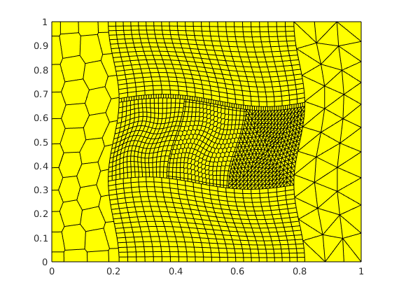
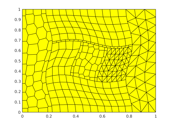
Linear Elasticity on Complex Grid¶

Generated from example_2D.m

We consider a case with a complex block-structured grid, in which each individual block is gridded using different grid types: curvilinear quadrilateral blocks, unstructured Voronoi grids, and triangular grids. The purpose of the example is to highlight the flexibility of the virtual element method.

mrstModule add vemmech

Set up the rock parameters and the grid¶

E  = 1;    % Young's modulus
nu = 0.3;  % Poisson's ratio

L = [1 1]; % Grid domain
dims = [16 16]; % The grid size

% Parameter used to twist the grid so that the Cartesian symmetries are
% broken and we can test the method on more irregular grid.
disturb = 0.03;

test_name = 'original_2D_test'; % list of test names to be found in file
                                % squareTest.
grid_type = 'mixed4'; % Run the script exploreSquareGrid to see the grids
                      % that have been set up to test this VEM code with
                      % respect to different grid features.

% We use the utility function squareTest to set up the problem, that is
% defining the load and boundary conditions.
[G, bc, test_cases] = squareTest('E', E, 'nu', nu, 'cartDims', dims, ...
                                 'L', L, 'grid_type', grid_type, 'disturb', disturb, ...
                                 'make_testcases', false, 'test_name', test_name);
G = computeGeometry(G);
clf, plotGrid(G);

% We recover the problem parameters using the structure test_cases
testcase = test_cases{1};
el_bc    = testcase.el_bc; % The boundary conditions
load     = testcase.load;  % The load
C        = testcase.C;     % The material parameters in Voigts notations

We assemble and solve the equations¶

[uVEM, extra] = VEM_linElast(G, C, el_bc, load);

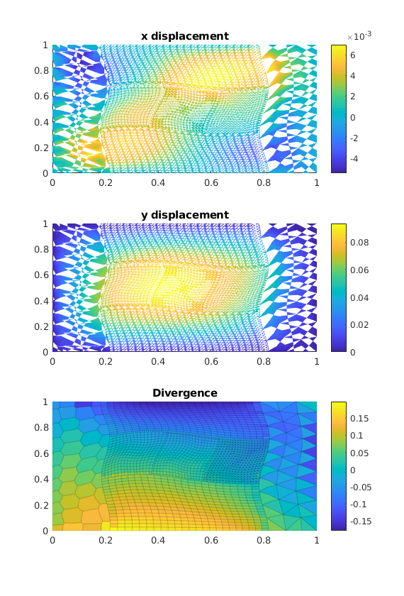
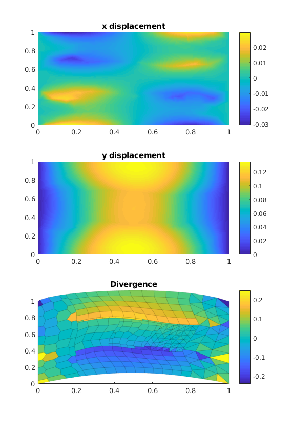
We plot the results¶

plotopts = {'EdgeAlpha', 0.0, 'EdgeColor', 'none'};
plotopts1 = {'EdgeAlpha', 0.1};
figure('Position',get(0, 'DefaultFigurePosition').*[1 1 1 2]);
subplot(3, 1, 1);
plotNodeData(G, uVEM(:, 1), plotopts{:}); colorbar();
title('x displacement');
subplot(3, 1, 2);
plotNodeData(G, uVEM(:, 2), plotopts{:}); colorbar();
title('y displacement');
subplot(3, 1, 3);
% We compute the divergence
vdiv = VEM2D_div(G);
mdiv = vdiv*reshape(uVEM', [], 1)./G.cells.volumes;
title('Divergence');
plotCellDataDeformed(G, mdiv, uVEM, plotopts1{:}); colorbar();

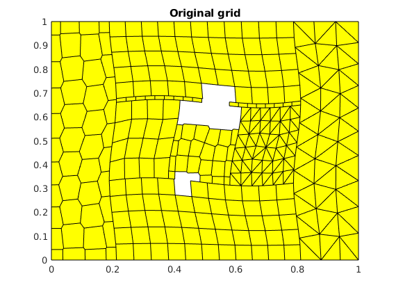
A short example solving linear elasticity on a complex grids¶

Generated from example_2D_complex_grid.m

Load required modules¶

mrstModule add vemmech

Define parameters¶

opt = struct('L'         , [1 1], ...
             'cartDims'  , [4 4], ...
             'grid_type' , 'square', ...
             'disturb'   , 0.02, ...
%parameter for disturbing grid
             'E'         , 4e7, ...
 %youngs modolo
             'nu'        , 0.44);% poiso ratio

make a mixed type of grid¶

G = squareGrid(opt.cartDims, opt.L, 'grid_type', 'mixed4', 'disturb', opt.disturb);
G = removeCells(G, [140 : 151, 233 : 235, 249 : 250, 93, 117 : 118]');
G = createAugmentedGrid(G);
G = computeGeometry(G);
figure()
plotGrid(G);
title('Original grid');

Find sides of domain¶

[Lx, Ly] = deal(opt.L(1), opt.L(2));
assert(G.griddim == 2);
x = [0, Lx];
bc = cell(4,1);
for i = 1 : 2
    faces = find(abs(G.faces.centroids(:, 1) - x(i)) < eps);
    bc{i} = addBC([], faces, 'pressure', 0);
    bc{i} = rmfield(bc{i}, 'type');
    bc{i} = rmfield(bc{i}, 'sat');
end
y = [0, Ly];
for i = 1 : 2
    faces = find(abs(G.faces.centroids(:, 2) - y(i)) < eps);
    bc{i + 2} = addBC([], faces, 'pressure', 0);
    bc{i + 2} = rmfield(bc{i + 2}, 'type');
    bc{i + 2} = rmfield(bc{i + 2}, 'sat');
end

for i = 1 : 4
    inodes = mcolon(G.faces.nodePos(bc{i}.face), G.faces.nodePos(bc{i}.face + 1) - 1);
    nodes = unique(G.faces.nodes(inodes));
    % Set up the boudary conditions.
    % Note that the fields 'faces' and 'uu_face' are not needed for VEM but
    % will become necessary when running other methods (such as MPSA)
    disp_bc = struct('nodes', nodes, ...
        'uu', 0, ...
        'faces', bc{i}.face, ...
        'uu_face', 0, ...
        'mask', true(numel(nodes), G.griddim));
    bc{i}.el_bc = struct('disp_bc', disp_bc, 'force_bc', []);
end

Set up the loading term¶

Gravity is our loading term

density = 3000; %kg/m^3
grav = 10; %gravity
load = @(x) - (grav*density)*repmat([0, 1], size(x, 1), 1);

Set up the displacement boundary condtions¶

% Set boundary displacement function to zero
bcdisp = @(x) x*0.0;

% Set up the boundary conditions for each side
bc_el_sides{1} = bc{1}; % x side is fixed
bc_el_sides{2} = bc{2}; % y side is fixed
bc_el_sides{3} = [];    % bottom  is free
bc_el_sides{4} = [];    % top is free

% Collect the displacement boundary conditions
nodes = [];
faces = [];
mask  = [];
for i = 1 : numel(bc)
    if (~isempty(bc_el_sides{i}))
        nodes = [nodes; bc_el_sides{i}.el_bc.disp_bc.nodes]; %#ok
        faces = [faces; bc_el_sides{i}.el_bc.disp_bc.faces]; %#ok
        mask  = [mask; bc_el_sides{i}.el_bc.disp_bc.mask];   %#ok
    end
end
disp_node  = bcdisp(G.nodes.coords(nodes, :));
disp_faces = bcdisp(G.faces.centroids(faces, :));
disp_bc = struct('nodes', nodes, 'uu', disp_node, 'faces', faces, 'uu_face', disp_faces, 'mask', mask);

Set up the force boundary conditions¶

% A force is applied on the top surface. It is discontinuous in the sense
% that it takes two different values on the left and on the right.
force = 50*barsa;
face_force = @(x) force*sign(x(:, 1) - opt.L(1)/2) + 100*barsa;
faces = bc{4}.face;
% Set up the force boundary structure,
% Note that the unit for the  force is  Pa/m^3.
force_bc = struct('faces', faces, 'force', bsxfun(@times, face_force(G.faces.centroids(faces, :)), [0 -1]));


% Final structure defining the boundary conditions
el_bc = struct('disp_bc', disp_bc, 'force_bc', force_bc);

Define the rock parameters¶

Ev = repmat(opt.E, G.cells.num, 1);
nuv = repmat(opt.nu*0 + 0.4, G.cells.num, 1);
C = Enu2C(Ev, nuv, G);

Assemble and solve the system¶

lsolve = @mldivide;
[uu, extra] = VEM_linElast(G, C, el_bc, load, 'linsolve', lsolve);

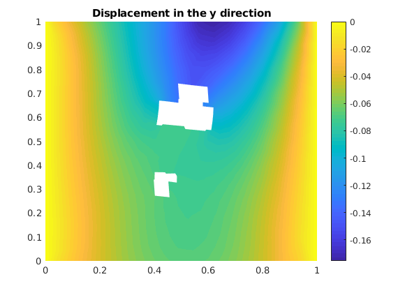
Plot displacement in y direction¶

plotopts = {'EdgeAlpha', 0.0, 'EdgeColor', 'none'};
plotopts1 = {'EdgeAlpha', 0.01};
figure()
plotNodeData(G, uu(:, 2), plotopts{ : });
colorbar();
title('Displacement in the y direction');

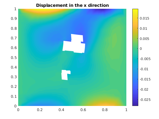
Plot the displacement in x direction¶

figure()
plotNodeData(G, uu(:, 1), plotopts{ : });
title('Displacement in the x direction');
colorbar();

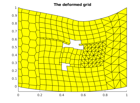
plot the deformed grid¶

figure()
fac = 1;
plotGridDeformed(G, uu*fac); axis tight
title('The deformed grid');

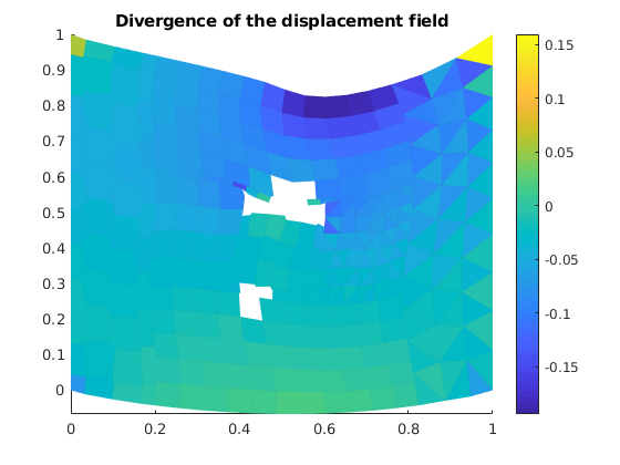
Calculate and plot the divergence¶

vdiv = VEM_div(G);
mdiv = vdiv*reshape(uu', [], 1)./G.cells.volumes;
figure()
plotCellDataDeformed(G, mdiv, uu*fac, plotopts1{ : }); axis tight
colorbar()
title('Divergence of the displacement field');

Calulate the stress and strain¶

op = extra;
stress = reshape(op.D*op.WC'*op.assemb'*reshape(uu', [], 1), 3, [])';

Example using three layers with different parameters in each layer¶

Generated from example_2D_layers.m

We set up a

mrstModule add vemmech

Set up the rock parameters and the grid¶

Use the utility function squareLayersTest to set up the problem. You may look at the documentation of this function and try the other settings presented there by modifying this example.

E  = [1; 10; 1];      % Define the Youngs moduli in the layers
nu = [0.3; 0.3; 0.3]; % Define the Poisson's ratio in the layers

zlayers = [0.3; 0.3; 0.3]; % Define the width of the layers.
zlayers = 1/sum(zlayers)*zlayers;
L    = [1 1];   % Define the domain size

% Define the grid type, for example 'mixed4'
grid_type = 'mixed4';
dims= [4 4];

% Define test case type. It determines the boundary conditions and the forces
test_name = 'hanging_rod_2D';
% Parameter used to twist the grid so that the Cartesian symmetries are
% broken and we can test the method on more irregular grid.
disturb = 0.042;

% The utility function squareLayersTest sets up the problem.
[G, bc, test_cases] = squareLayersTest('E', E, 'nu', nu, 'zlayers', ...
    zlayers, 'cartDims', dims, 'L', L, 'grid_type', grid_type, 'disturb', ...
    disturb, 'make_testcases', false, 'test_name', test_name);
G = computeGeometry(G);
figure,
plotGrid(G);

% We recover the problem parameters using the structure test_cases
testcase = test_cases{1};
el_bc    = testcase.el_bc; % The boundary conditions
load     = testcase.load;  % The load
C        = testcase.C;     % The material parameters in Voigts notations

We assemble and solve the equations¶

[uVEM, extra] = VEM_linElast(G, C, el_bc, load);

We plot the results¶

plotopts = {'EdgeAlpha', 0.0, 'EdgeColor', 'none'};
plotopts1 = {'EdgeAlpha', 0.1};
figure('Position',get(0, 'DefaultFigurePosition').*[1 1 1 2]);
subplot(3, 1, 1);
plotNodeData(G, uVEM(:, 1), plotopts{:}); colorbar();
title('x displacement');
subplot(3, 1, 2);
plotNodeData(G, uVEM(:, 2), plotopts{:}); colorbar();
title('y displacement');
subplot(3, 1, 3);
% We compute the divergence
vdiv = VEM2D_div(G);
mdiv = vdiv*reshape(uVEM', [], 1)./G.cells.volumes;
title('Divergence');
plotCellDataDeformed(G, mdiv, uVEM, plotopts1{:}); colorbar(); axis tight

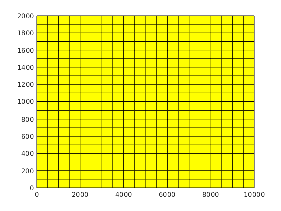
Example of poro-elastic problem¶

Generated from example_poroelasticity.m

This example sets up a poro-elastic problem which mimics a slice of the overburden, with an infinite horizontal well in an aquifer at the bottom of the domain. The poro-elastic equations are set up together with linear explicitely. At the end we simulate the same case by using the poro-elastic solver and compare with the results predicted by linear elasticity. More examples can be generated by modifying the parameters sent to the function squareTest.m,

mrstModule add incomp vemmech

Define the grid and rock parameters¶

opt = struct( 'L'         , [10000 2000], ...
              'cartDims'  , [20 20]*1,    ...
              'grid_type' , 'square',     ...
              'disturb'   , 0.0,          ...
% Parameter for disturbing grid
              'E'         , 1e9,          ...
% Young's modulus
              'nu'        , 0.2);             % Poisson's ratio


G = cartGrid(opt.cartDims, opt.L);
if (opt.disturb > 0)
    G = twister(G, opt.disturb);
end
G = createAugmentedGrid(G);
G = computeGeometry(G);

Ev  = repmat(opt.E, G.cells.num, 1);
nuv = repmat(opt.nu, G.cells.num, 1);
C   = Enu2C(Ev, nuv, G);

figure()
clf,
plotGrid(G)

Set up gravity as the loading term¶

gravity reset on
density = 3000; % in kg/m^3
grav    = norm(gravity());   % gravity
load    = @(x) -(grav*density)*repmat([0, 1], size(x, 1), 1);

Set up the displacement boundary conditions¶

oside = {'Left', 'Right', 'Back', 'Front'};
bc = cell(4, 1);
for i = 1 : numel(oside);
    bc{i} = pside([], G, oside{i}, 0);
    bc{i} = rmfield(bc{i}, 'type');
    bc{i} = rmfield(bc{i}, 'sat');
end
% Find the nodes for the different sides and set the boundaray conditions for
% elastisity.
for i = 1 : 4
    inodes = mcolon(G.faces.nodePos(bc{i}.face), G.faces.nodePos(bc{i}.face + 1) - 1);
    nodes = unique(G.faces.nodes(inodes));
    disp_bc = struct('nodes'   , nodes,      ...
                     'uu'      , 0,          ...
                     'faces'   , bc{i}.face, ...
                     'uu_face' , 0,          ...
                     'mask'    , true(numel(nodes), G.griddim));
    bc{i}.el_bc = struct('disp_bc', disp_bc, 'force_bc', []);
end
bcdisp = @(x) x*0.0; % Boundary displacement function set to zero.
% Setup diriclet boundary conditions at selected sides
%
% On the left and right-hand sides, zero displacement is imposed in the x
% direction, and free in the y direction. This is done by using masks.
bc_el_sides{1} = bc{1};
bc_el_sides{1}.el_bc.disp_bc.mask(:, 2) = false;
bc_el_sides{2} = bc{2};
bc_el_sides{2}.el_bc.disp_bc.mask(:, 2) = false;
% Zero displacement is imposed in the y direction at the bottom, free
% displacement at the top.
bc_el_sides{3} = bc{3};
bc_el_sides{3}.el_bc.disp_bc.mask(:, 1) = false;
bc_el_sides{4} = [];

% Collect the displacement boundary conditions
nodes = [];
faces = [];
mask = [];
for i = 1 : numel(bc)
    if(~isempty(bc_el_sides{i}))
        nodes = [nodes; bc_el_sides{i}.el_bc.disp_bc.nodes]; %#ok
        faces = [faces; bc_el_sides{i}.el_bc.disp_bc.faces]; %#ok
        mask  = [mask; bc_el_sides{i}.el_bc.disp_bc.mask]; %#ok
    end
end
disp_node = bcdisp(G.nodes.coords(nodes, :));
disp_faces = bcdisp(G.faces.centroids(faces, :));
disp_bc = struct('nodes', nodes, 'uu', disp_node, 'faces', faces, 'uu_face', disp_faces, 'mask', mask);

Set up the force boundary conditions¶

% A force is applied on the top surface.
sigma = opt.L(2)/10;
force = 100*barsa;
face_force = @(x) force*exp(-(((x(:, 1) - opt.L(1)/2))./sigma).^2) + 10*barsa;
faces = bc{4}.face;
% Set up the force boundary structure
% Note that the unit for the force is in units Pa/m^3
force_bc = struct('faces', faces, 'force', bsxfun(@times, face_force(G.faces.centroids(faces, :)), [0 -1]));


% Final structure for the  boundary conditions
el_bc = struct('disp_bc', disp_bc, 'force_bc', force_bc);

Assemble and solve the system¶

[uu, extra] = VEM_linElast(G, C, el_bc, load);

% We retrieve the discrete operators that have been assembled
As        = extra.disc.A;     % Global stiffness matrix
div       = extra.disc.div;   % Divergence operator
gradP     = extra.disc.gradP; % Gradient operator (dual of div)
isdirdofs = extra.disc.isdirdofs; % Degrees of freedom where in fact
                                  % Dirichlet boundary conditions are imposed.
rhs_s     = extra.disc.rhs;   % Right-hand side
Vdir      = extra.disc.V_dir; %
ind_s     = [1 : size(As, 1)]';%#ok

Set up the parameters for the flow part¶

perm = 1*darcy*ones(G.cartDims);
perm(:, floor(G.cartDims(2)/5) : end) = 1*milli*darcy;
rock = struct('perm', reshape(perm, [], 1),     ...
              'poro', 0.1*ones(G.cells.num, 1), ...
              'alpha', ones(G.cells.num, 1)); % Rock parameters
fluid = initSingleFluid('mu', 1*centi*poise, 'rho', 1000); % Fluid parameters
rock.cr = 1e-4/barsa; % Fluid compressibility
T = computeTrans(G, rock); % Compute the transmissibilities
pv = poreVolume(G, rock); % Compute the pore volume
pressure = 100*barsa*ones(G.cells.num, 1); % Initial pressure
% Set up the initial state for the flow.
state = struct('pressure', pressure, 's', ones(G.cells.num, 1), 'flux', zeros(G.faces.num, 1));
% Set up a well structure for the fluid injection and also boundary
% conditions for the flow.
mcoord = [5000 200];
[dd, wc] = min(sum(bsxfun(@minus, G.cells.centroids, mcoord).^2, 2));
W = addWell([], G, rock, wc, 'type', 'bhp', 'val', 3000*barsa);
bc_f = pside([], G, 'Front', 10*barsa);
fbc = addFluidContribMechVEM(G, bc_f, rock, isdirdofs);

Set up matrix for mechanics and flow¶

Use a TPFA solver for weakly compressible flow. From the output we retrieve the operators for the fluid.

dt = day; % time step.
state = lincompTPFA(dt, state, G, T, pv, fluid, rock, 'MatrixOutput', true, 'wells', W, 'bc', bc_f);

Af    = state.A;   % Global matrix for the flow solver
orhsf = state.rhs; % Right-hand side for the flow equations (includes well)
ct    = state.ct;  % Compressibility coefficient
ind_f = [ind_s(end) + 1 : ind_s(end) + G.cells.num]';%#ok

% x denotes the global unknown (displacement + pressure)
x = zeros(ind_f(end), 1);
x(ind_f) = pressure;
p = pressure;

uu0 = uu;            % Solution from linear elasticity
u_tmp = reshape(uu', [], 1);
x(1 : ind_s(end)) = u_tmp(~isdirdofs);
u = zeros(numel(isdirdofs), 1);
rhsf = zeros(size(orhsf));
plotops = {'EdgeColor', 'none'};
fac = rock.poro(1);

% Assemble the matrix for the global system, mechanics + flow
zeromat = sparse(size(Af, 1) - G.cells.num, size(div, 2));
SS = [As, [fac*(-gradP), zeromat']; [fac*div; zeromat], ct + dt*Af];

Time loop¶

Set up bigger figures

df = get(0, 'DefaultFigurePosition');
figure(1); set(1, 'Position', df.*[0.8, 1, 3, 1]); clf
figure(2); set(2, 'Position', df.*[1, 1, 3, 1]); clf

t = 0;
end_time = 10*dt;
while t < end_time
    t = t + dt;
    % We update the right-hand side for the fluid (divergence term comes
    % from mechanics).
    rhsf(1 : G.cells.num) = orhsf(1 : G.cells.num)*dt + ct(1 : G.cells.num, 1 : G.cells.num)*p + fac*div*x(ind_s);
    rhsf(G.cells.num + 1 : end) = orhsf(G.cells.num + 1 : end);
    rhs = [rhs_s - fbc; rhsf];

    % Solve the system
    x = SS\rhs;

    % Retrieve pressure and displacement
    p = x(ind_f); % retrieve pressure
    u(isdirdofs) = Vdir(isdirdofs);
    u(~isdirdofs) = x(ind_s); % retrieve displacement
    uu = reshape(u, G.griddim, [])';

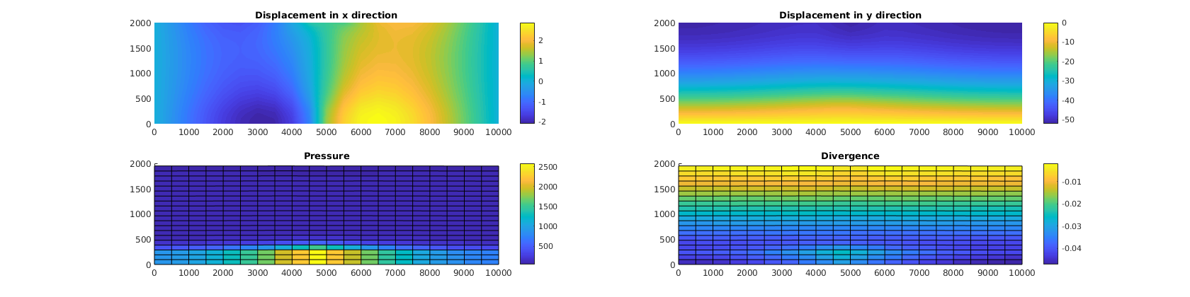
    % Plot absolute results from poromechanics
    figure(1)
    subplot(2, 2, 1), cla
    plotNodeData(G, uu(:, 1), plotops{ : }); colorbar;
    title('Displacement in x direction')
    subplot(2, 2, 2), cla
    plotNodeData(G, uu(:, 2), plotops{ : }); colorbar;
    title('Displacement in y direction')
    subplot(2, 2, 3), cla
    plotCellDataDeformed(G, p/barsa, uu); colorbar;
    title('Pressure')
    subplot(2, 2, 4), cla
    ovdiv = extra.disc.ovol_div;
    mdiv = ovdiv*reshape(uu', [], 1)./G.cells.volumes;
    plotCellDataDeformed(G, mdiv, uu); colorbar();
    title('Divergence')

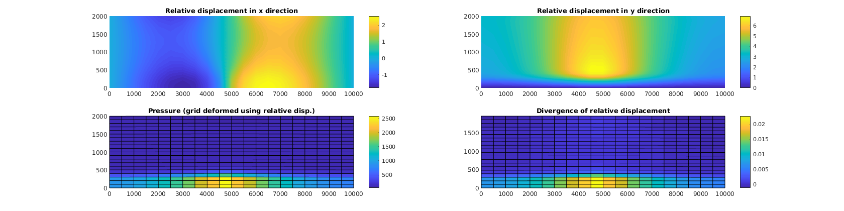
    % Plot difference from results predicted by linear elasticity
    figure(2)
    uur = uu - uu0;
    subplot(2, 2, 1), cla
    plotNodeData(G, uur(:, 1), plotops{ : }); colorbar;
    title('Relative displacement in x direction')
    subplot(2, 2, 2), cla
    plotNodeData(G, uur(:, 2), plotops{ : }); colorbar;
    title('Relative displacement in y direction')
    subplot(2, 2, 3), cla
    plotCellDataDeformed(G, p/barsa, uur); colorbar;
    title('Pressure (grid deformed using relative disp.)')
    axis tight
    subplot(2, 2, 4), cla
    ovdiv = extra.disc.ovol_div;
    mdiv = ovdiv*reshape(uur', [], 1)./G.cells.volumes;
    plotCellDataDeformed(G, mdiv, uu); colorbar();
    title('Divergence of relative displacement')
    axis tight
    %pause(0.01);

end

Parameters:	dim – Dimension
Returns:	disp names

vemmech: Mechanics for general grids using the virtual element method¶

Examples¶

Compaction test case in 2D¶

Define the fluid and rock parameters and set up the grid.¶

Setup the loads and the boundary conditions¶

Assemble and solve the system¶

Computation of the analytical solution¶

Comparison plots¶

Compaction test case 3D¶

Load required modules¶

Define the fluid and rock parameters and set up the grid.¶

Setup the loads and the boundary conditions¶

Assemble and solve the system¶

Compute the analytical solution¶

Comparison plots¶

Linear Elasticity on Complex Grid¶

Set up the rock parameters and the grid¶

We assemble and solve the equations¶

We plot the results¶

A short example solving linear elasticity on a complex grids¶

Load required modules¶

Define parameters¶

make a mixed type of grid¶

Find sides of domain¶

Set up the loading term¶

Set up the displacement boundary condtions¶

Set up the force boundary conditions¶

Define the rock parameters¶

Assemble and solve the system¶

Plot displacement in y direction¶

Plot the displacement in x direction¶

plot the deformed grid¶

Calculate and plot the divergence¶

Calulate the stress and strain¶

Example using three layers with different parameters in each layer¶

Set up the rock parameters and the grid¶

We assemble and solve the equations¶

We plot the results¶

Example of poro-elastic problem¶

Define the grid and rock parameters¶

Set up gravity as the loading term¶

Set up the displacement boundary conditions¶

Set up the force boundary conditions¶

Assemble and solve the system¶

Set up the parameters for the flow part¶

Set up matrix for mechanics and flow¶

Time loop¶

`vemmech`: Mechanics for general grids using the virtual element method¶