`re-mpfa`: Richards’ equation with multi-point flux¶

arithmeticMPFA_hydHead(krw, G_struct, bc_struct, hydHead, zetaCells, zetaFaces)¶

Computes the arithmetic average of the relative permeability

Synopsis:

krwAr = arithmeticMPFA_hydHead(krw,G_struct,bc_struct,hydHead,zetaCells,zetaFaces)

Parameters:

krw – Function, relative permeability function krw = krw(psi)
G_struct – Structure, Grid structure from MRST
bc_struct – Structure, Boundary conditions structure from MRST
hydHead – Vector, containing the values of hydraulic head. This vector must have a length equal to G_struct.cells.num
zetaCells – Vector, containing the values of the elevation head at the cell centers. This vector must have a length equal to G_struct.cells.num
zetaFaces –

Vector, contaning the values of the elevation head at

the faces centroids. This vector must have a length equal to G_struct.faces.num

RETURNS:

krwAr - Vector, containing the arithmetic averaged relative

permeabilities at the faces. This vector will have a lenght equal to G_struct.faces.num

newtonSolver(h_ad, h_eq, timeCum, dt, maxTolPresHead, maxIter)¶

Newton-AD (Automatic Differentiation) solver

Synopsis:

[h_ad,h_m0,iter,timeCum,tf] = newtonSolver(h_ad,h_eq,timeCum,dt,maxTolPresHead,maxIter)

Parameters:

h_ad – AD variable, hydraulic head (primary variable)
h_eq – Function, hydraulic head discrete equation
timeCum – Scalar, cumulative time
dt – Scalar, time step
maxTolPresHead – Scalar, maximum tolerance of pressure head ~ 1 [cm]
maxIter –
Scalar, maximum iteration number ~ 10

RETURNS:

h_ad - AD variable, updated hydraulic head AD varible h_m0 - Vector, containing pressure head of the last

iteration level

iter - Scalar, number of iterations timeCum - Scalar, updated cumulative time tf - Scalar, computational time

timeStepping(dt, dt_min, dt_max, simTime, timeCum, iter, printTimes, printCounter, lowerOptIterRange, upperOptIterRange, lowerMultFactor, upperMultFactor)¶

Calculates the next time step dt

timeStepping determines the next time step according to the number of iterations from the last step in the following way.

If the number of iterations is less (or equal) than the lower optimal range (lowerOptIterRange), it will increase the time step. In other words, it will multiply the previous time step by a factor of lowerMultFactor.

On the other hand, if the number of iterations is greater (or equal) than the upper optimal range (upperOptIterRange), it will decrease the time step. Hence, it will multiply the previous time step by a factor of upperMultFactor.

Finally, if the number of iterations lies within the lower and upper

If the time step lies withing the optimal range, the previous time step will remain unchanged.

Synopsis:

[dt,printCounter] = timeStepping(dt,dt_min,dt_max,simTime,timeCum,iter,printTimes,printCounter,...
                                 lowerOptIterRange,upperOptIterRange,lowerMultFactor,upperMultFactor)

Parameters:

dt – Scalar, previous time step
dt_min – Scalar, minimum time step
dt_max – Scalar, maximum time step
simTime – Scalar, final simulation time
timeCum – Scalar, current simulation time
iter – Scalar, number of iterations of the current time
printTimes – Vector, containing printing times
printCounter – Scalar, counter of printed times
lowerOptIterRange – Scalar, lower optimal iteration range
upperOptIterRange – Scalar, upper optimal iteration range
lowerMultFactor – Scalar, lower multiplication factor
upperMultFactor –
Scalar, upper multiplication factor

RETURNS:

dt - Scalar, time step for the next time level printCounter - Scalar, updated counter of printed times

upstreamMPFA_hydHead(krw, F, boundF, G_struct, bc_struct, bc_val, hydHead, zetaCells, zetaFaces)¶

Computes the upstream weighting of the relative permeability

Synopsis:

krwAr = upstreamMPFA_hydHead(krw,gradF,boundF,G_struct,bc_struct,bc_val,hydHead,zetaCells,zetaFaces)

Parameters:

krw – Function, relative permeability function krw = krw(psi)
F – Function, MPFA discrete operator that acts on the hydraulic head
boundF – Function, MPFA discrete operator that acts on bc_val
G_struct – Structure, Grid structure from MRST
bc_struct – Structure, Boundary conditions structure from MRST
bc_val – Vector, containing the values of boundary conditions. This vector must have a length equal to G_struct.faces.num
hydHead – Vector, containing the values of hydraulic head. This vector must have a length equal to G_struct.cells.num
zetaCells – Vector, containing the values of the elevation head at the cell centers. This vector must have a length equal to G_struct.cells.num
zetaFaces –

Vector, contaning the values of the elevation head at

the faces centroids. This vector must have a length equal to G_struct.faces.num

RETURNS:

krwUp - Vector, containing the upstream weighted relative

permeabilities at the faces. This vector will have a lenght equal to G_struct.faces.num

Examples¶

Three-dimensional water evaporation process¶

Generated from waterEvaporation3D.m

This code is an implementation of the mixed-based form of the Richards’ Equation in a three-dimensional domain using Automatic Differentiation from MRST (see http://www.sintef.no/projectweb/mrst/). The grid is set to be cartesian and structured. For the spatial discretization we use cell-centered finite volume method with multi-point flux approximation from https://github.com/keileg/fvbiot. For the time derivative we use the modified picard iteration proposed in: http://onlinelibrary.wiley.com/doi/10.1029/92WR01488/abstract. We decided to use the hydraulic head as primary variable instead of the classical approach (the pressure head) in order to avoid any inconsistency in the gravity contribution. The intrisic permeability at the faces are approximated using harmonic average while the relative permeabilities are upstream weighted. The problem of interest is the instanteous evaporation of water through the top boundary, which is assumed to be constant. All the boundary conditions are set as no flux, except the top boundary which is set as constant flux. We expect a decrease in pressure as well as saturation as time evolves.

Mass Conservation

$\frac{\partial \theta}{\partial t} + \nabla \cdot \vec{q} = 0$

Multiphase Darcy’s Law

$\vec{q} = -k \frac{\rho g}{\mu} k_{rw} \nabla h$

Mass Conservation

$\frac{V_{\{c\}}}{\Delta t} \left( \theta_{\{c\}}^{n+1,m} + C_{\{c\}}^{n+1,m} \left( h_{\{c\}}^{n+1,m+1} - h_{\{c\}}^{n+1,m} \right) - \theta_{\{c\}}^n \right) + \left[ \mathbf{div} \left( \vec{q}_{\{f\}} \right) \right]_{\{c\}} = 0$

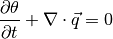
Multiphase Darcy’s Law

$\vec{q}_{\{f\}} = \frac{\rho g}{\mu} \left[ \mathbf{upstr} \left( {k_{rw}}_{\{c\}}^{n+1,m} \right) \right]_{\{f\}} \left( \left[ \mathbf{F} \left( h_{\{c\}}^{n+1,m+1}\right)\right]_{\{f\}} + \left[ \mathbf{boundF} \left(b_{\{f\}} \right) \right]_{\{f\}} \right)$

where

is the soil moisture content,

is the residual moisture content and

,

and

are the van Genuchten’s parameters.

Clearing workspace and cleaning console¶

clear; clc();

Importing modules¶

mrstModule add re-mpfa fvbiot

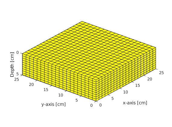
Setting up the Grid¶

nx = 20;              % Cells in x-direction
ny = 20;              % Cells in y-direction
nz = 10;              % Cells in z-direction
Lx = 25;              % Lenght in x-direction
Ly = 25;              % Length in y-direction
Lz = 5;               % Length in z-direction
G = computeGeometry(cartGrid([nx,ny,nz],[Lx,Ly,Lz])); % computing geometry
V = G.cells.volumes;  % Cell volumes

% Plotting Grid
figure(1); plotGrid(G);
xlabel('x-axis [cm]'); ylabel('y-axis [cm]'); zlabel('Depth [cm]');
axis tight; pbaspect([1,1,0.25]); view([-51,26]);

Fluid Properties¶

rho = 1;                    % [g/cm^3] water density
mu = 0.01;                  % [g/cm.s] water viscosity
g = 980.6650;               % [cm/s^2] gravity acceleration

Rock Properties¶

K_sat = 0.00922;            % [cm/s] saturated hydraulic conductivity
k = (K_sat*mu)/(rho*g);     % [cm^2] intrinsic permeability
rock.perm = repmat([k, k, k], [G.cells.num, 1]); % creating perm structure

Van Genuchten Parameters¶

alpha = 0.0335;       % [1/cm] Equation parameter
nVan = 2;             % [-]    Equation parameter
mVan = 1-(1/nVan);    % [-]    Equation parameter
theta_s = 0.368;      % [-]    Saturation soil moisture
theta_r = 0.102;      % [-]    Residual soil moisture

Boundary and Initial Conditions¶

% Extracting Grid information
zCentr = G.cells.centroids(:,3);   % centroids of cells in z-direction
zFaces = G.faces.centroids(:,3);   % centroids of faces in z-direction
zetaCentr = Lz - zCentr;           % centroids of cells of elev. head
zetaFaces = Lz - zFaces;           % centroids of faces of elev. head

% Determining boundary indices
x_min = find(G.faces.centroids(:,1) == 0);             % west bound indices
x_max = find(G.faces.centroids(:,1) > 0.9999*Lx & ...
             G.faces.centroids(:,1) < 1.0001*Lx );     % east bound indices

y_min = find(G.faces.centroids(:,2) == 0);             % south bound indices
y_max = find(G.faces.centroids(:,2) > 0.9999*Ly & ...
             G.faces.centroids(:,2) < 1.0001*Ly );     % north bound indices

z_min = find(G.faces.centroids(:,3) == 0);             % top bound indices
z_max = find( G.faces.centroids(:,3) > 0.9999*Lz & ...
              G.faces.centroids(:,3) < 1.0001*Lz );    % bottom bound indices

% Boundary values
fluxW = 0;                                   % [cm^3/s] West boundary
fluxE = 0;                                   % [cm^3/s] East boundary
fluxS = 0;                                   % [cm^3/s] South boundary
fluxN = 0;                                   % [cm^3/s] North boundary
topCellsNum = G.cells.num/nz;                % number of cells of the top boundary
topArea = sum(G.faces.areas(z_min));         % [cm^2] total area of the top boundary
evapVel  = -0.75 * (1/3600);                 % [cm/s] evaporation velocity
evapFlux = evapVel * topArea;                % [cm^3/s] evaporation flux
% fluxTop_flux is the "artificial flux" that we have to pass to the
% bcFlow_flux structure. In this case we applied a constant flux that leaves
% the system through the top layer. We need to multiply by (mu*g/rho) and
% divide by the number of cells in order to assign a local contribution
fluxT = -evapFlux * (mu/(rho*g)) / topCellsNum;% [cm^3/s] Top boundary
fluxB = 0;                                   % [cm^3/s] Bottom boundary

% Creating the boundary structure
bc = addBC([], x_min, 'flux', fluxW);       % setting West boundary
bc = addBC(bc, x_max, 'flux', fluxE);       % setting East boundary
bc = addBC(bc, y_min, 'flux', fluxS);       % setting South boundary
bc = addBC(bc, y_max, 'flux', fluxN);       % setting North boundary
bc = addBC(bc, z_min, 'flux', fluxT);       % setting Top boundary
bc = addBC(bc, z_max, 'flux', fluxB);       % setting Bottom boundary

% Setting the boundary values vector
bc_val = zeros(G.faces.num, 1);             % initializing
bc_val(x_min) = fluxW;                      % assigning West boundary
bc_val(x_max) = fluxE;                      % assigning East boundary
bc_val(y_min) = fluxS;                      % assigning South boundary
bc_val(y_max) = fluxN;                      % assigning North boundary
bc_val(z_min) = fluxT;                      % assigning Top boundary
bc_val(z_max) = fluxB;                      % assigning Bottom boundary

% Initial Condition
psi_init = -1;                              % [cm] Pressure head initial cond.
h_init = psi_init + zetaCentr;              % [cm] Hydraulic head initial cond.

Calling MPFA routine¶

mpfa_discr = mpfa(G,rock,[],'bc',bc,'invertBlocks','matlab');

Creating discrete mpfa-operators¶

F = @(x) mpfa_discr.F * x;                  % flux discretization
boundF = @(x) mpfa_discr.boundFlux * x;     % boundary discretization
divf = @(x) mpfa_discr.div * x;             % divergence

Creating AD variable¶

h_ad = initVariablesADI(h_init);

Water retention curves¶

% Boolean function to determine if we are in the unsat or sat zone
isUnsat = @(x) x < 0;

% Water content
theta= @(x)     isUnsat(x) .* ((theta_s - theta_r) ./ ...
                (1 + (alpha .* abs(x)).^nVan).^mVan + theta_r ) + ...
                ~isUnsat(x) .* theta_s;

% Specific Moisture Capacity
cVan= @(x)      isUnsat(x) .* ((mVan .* nVan .* x .* (theta_r-theta_s) .* ...
                alpha.^nVan .* abs(x).^(nVan-2) ) ./ ...
                (alpha^nVan .* abs(x).^nVan + 1).^(mVan+1)) + ...
                ~isUnsat(x) .* 0;

% Relative permeability
krw= @(x)       isUnsat(x) .* ((1 - (alpha .* abs(x)).^(nVan-1) .* ...
                (1 + (alpha .* abs(x)).^nVan).^(-mVan)).^2 ./ ...
                (1 + (alpha .* abs(x)).^nVan).^(mVan./2)) + ...
                ~isUnsat(x) .* 1;

Time parameters¶

simTime = 3250;         % [s]    final simulation time
dt_init = 0.01;         % [s]    initial time step
dt_min = 0.01;          % [s]    minimum time step
dt_max = 1000;          % [s]    maximum time step
lowerOptIterRange = 3;  % [iter] lower optimal iteration range
upperOptIterRange = 7;  % [iter] upper optimal iteration range
lowerMultFactor = 1.3;  % [-]    lower multiplication factor
upperMultFactor = 0.7;  % [-]    upper multiplication factor
dt = dt_init;           % [s]    initializing time step
timeCum = 0;            % [s]    initializing cumulative time
currentTime = 0;        % [s]    current time

Printing parameters¶

printLevels = 30;       % number of printing levels
printTimes = ((simTime/printLevels):(simTime/printLevels):simTime)';   % printing times
printCounter = 1;       % initializing printing counter
exportCounter = 1;      % intializing exporting counter

Discrete equations¶

% Arithmetic Average
krwAr = @(h_m0) arithmeticMPFA_hydHead(krw,G,bc,h_m0,zetaCentr,zetaFaces);

% Darcy Flux
q = @(h,h_m0)  (rho.*g./mu) .* krwAr(h_m0) .* (F(h) + boundF(bc_val));

% Mass Conservation
hEq = @(h,h_n0,h_m0,dt) (V./dt) .* (...
                                theta(h_m0-zetaCentr) + ...
                                cVan(h_m0-zetaCentr) .* (h - h_m0) - ...
                                theta(h_n0-zetaCentr) ...
                                ) + divf(q(h,h_m0));

Creating solution structure¶

sol = struct('time',[],'h',[],'psi',[],'zeta',[],'theta',[],'flux',[],...
             'iter',[],'residual',[],'cpuTime',[]);

% We need to initialize doubles and cells to store the values in sol
t = zeros(printLevels,1);            % Cummulative time
h_cell = cell(printLevels,1);        % Hydraulic Heads
psi_cell = cell(printLevels,1);      % Pressure Heads
zeta_cell = cell(printLevels,1);     % Elevation Heads
theta_cell = cell(printLevels,1);    % Water content
flux_cell = cell(printLevels,1);     % Fluxes
residual = cell(printLevels,1);      % Residuals
iterations = zeros(printLevels,1);   % Iterations
cpuTime = zeros(printLevels,1);      % CPU time

Solving via Newton¶

while timeCum < simTime

    % Newton parameters
    maxTolPresHead = 1; % [cm] maximum absolute tolerance of pressure head
    maxIter = 10;       % maximum number iterations

    % Calling Newton solver
    [h_ad,h_m0,iter,timeCum,tf] = newtonSolver(h_ad,hEq,timeCum,...
                                               dt,maxTolPresHead,maxIter);

    % Calling Time stepping routine
    [dt,printCounter] = timeStepping(dt,dt_min,dt_max,simTime,...
                           timeCum,iter,printTimes,printCounter,...
                           lowerOptIterRange,upperOptIterRange,...
                           lowerMultFactor,upperMultFactor);

    % Storing solutions at each printing time
    if timeCum == printTimes(exportCounter)
        h_cell{exportCounter,1} = h_ad.val;
        psi_cell{exportCounter,1} = h_ad.val - zetaCentr;
        zeta_cell{exportCounter,1} = zetaCentr;
        theta_cell{exportCounter,1} = theta(h_ad.val - zetaCentr);
        flux_cell{exportCounter,1} = q(h_ad.val,h_m0);
        t(exportCounter,1) = timeCum;
        iterations(exportCounter,1) = iter-1;
        cpuTime(exportCounter,1) = tf;
        exportCounter = exportCounter + 1;
    end

end

Time: 0.010 [s]        Iter: 1         Error: 3.556265e-01 [cm]
Time: 0.023 [s]        Iter: 1         Error: 3.806415e-01 [cm]
Time: 0.040 [s]        Iter: 1         Error: 4.757754e-01 [cm]
Time: 0.062 [s]        Iter: 1         Error: 6.222749e-01 [cm]
Time: 0.090 [s]        Iter: 1         Error: 5.877094e-01 [cm]
Time: 0.128 [s]        Iter: 1         Error: 3.852761e-01 [cm]
Time: 0.176 [s]        Iter: 1         Error: 1.626544e-01 [cm]
Time: 0.239 [s]        Iter: 1         Error: 5.180366e-02 [cm]
...

Storing results in the sol structure¶

sol.time = t;           sol.h = h_cell;             sol.psi = psi_cell;
sol.zeta = zeta_cell;   sol.theta = theta_cell;     sol.flux = flux_cell;
sol.iter = iterations;  sol.residual = residual;    sol.cpuTime = cpuTime;

fprintf('\n sol: \n'); disp(sol);  % printing solutions in the command window

sol:
        time: [30×1 double]
           h: {30×1 cell}
         psi: {30×1 cell}
        zeta: {30×1 cell}
       theta: {30×1 cell}
        flux: {30×1 cell}
...

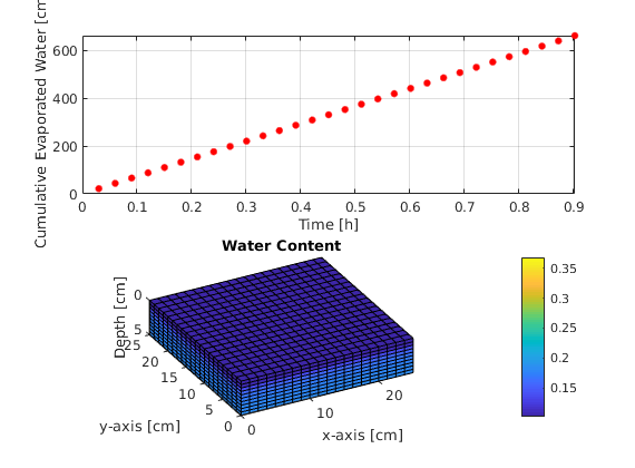
Cumulative evaporated water and water content reduction¶

figure(3);

% Determining cumulative water flux
waterProd = zeros(printLevels,1);
for ii=1:printLevels
    waterProd(ii) = waterProd(ii) + sum(sol.flux{ii,1}(z_min))*sol.time(ii);
end

% Plotting cumulative flux and water content
for ii=1:printLevels
    subplot(2,1,1)
    plot(sol.time(ii)/3600,abs(waterProd(ii)),'.r','MarkerSize',15);
    hold on; grid on; axis tight;
    xlabel('Time [h]'), ylabel('Cumulative Evaporated Water [cm^3]');
    xlim([0 simTime/3600]); ylim([0 abs(waterProd(end))]);

    subplot(2,1,2)
    plotCellData(G,sol.theta{ii});
    xlabel('x-axis [cm]'), ylabel('y-axis [cm]'), zlabel('Depth [cm]');
    xlim([0 Lx]); ylim([0 Ly]); zlim([0 Lz]); axis equal;
    view([-28 28]); shading faceted;
    box on; pbaspect([1 1 2.5]);
    t_h1=handle(text('Units','normalized',...
   % Use [%] of the axis length
                     'Position',[1,0.9,1],...
   % Position of text
                     'EdgeColor','w'));          % Textbox
    t_h1.String=sprintf('Time: %2.2f [h]',sol.time(ii)/3600); % print "time" counter
    title('Water Content'); pause(0.5);
    colorbar; caxis([theta_r theta_s]);
    t_h1.String =[];
end

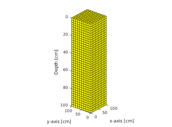
Pseudo One-Dimensional water infiltration process¶

Generated from waterInfiltration1D.m

This code is an implementation of the mixed-based form of the Richards’ Equation in a pseudo-one dimensional domain using Automatic Differentiation from MRST (see http://www.sintef.no/projectweb/mrst/). The grid is set to be cartesian and structured. For the spatial discretization we use cell-centered finite volume method with multi-point flux approximation from https://github.com/keileg/fvbiot. For the time derivative we use the modified picard iteration proposed in: http://onlinelibrary.wiley.com/doi/10.1029/92WR01488/abstract. We decided to use the hydraulic head as primary variable instead of the classical approach (the pressure head) in order to avoid any inconsistency in the gravity contribution. The intrisic permeability at the faces are approximated using harmonic average while the relative permeabilities are upstream weighted. The problem of interest is the vertical infiltration of water (from top to bottom). For the boundary conditions we use constant

at top and bottom of the domain and no flux elsewhere.

Mass Conservation

$\frac{\partial \theta}{\partial t} + \nabla \cdot \vec{q} = 0$

Multiphase Darcy’s Law

$\vec{q} = -k \frac{\rho g}{\mu} k_{rw} \nabla h$

Mass Conservation

$\frac{V_{\{c\}}}{\Delta t} \left( \theta_{\{c\}}^{n+1,m} + C_{\{c\}}^{n+1,m} \left( h_{\{c\}}^{n+1,m+1} - h_{\{c\}}^{n+1,m} \right) - \theta_{\{c\}}^n \right) + \left[ \mathbf{div} \left( \vec{q}_{\{f\}} \right) \right]_{\{c\}} = 0$

Multiphase Darcy’s Law

$\vec{q}_{\{f\}} = \frac{\rho g}{\mu} \left[ \mathbf{upstr} \left( {k_{rw}}_{\{c\}}^{n+1,m} \right) \right]_{\{f\}} \left( \left[ \mathbf{F} \left( h_{\{c\}}^{n+1,m+1}\right)\right]_{\{f\}} + \left[ \mathbf{boundF} \left(b_{\{f\}} \right) \right]_{\{f\}} \right)$

where

is the soil moisture content,

is the residual moisture content and

,

and

are the van Genuchten’s parameters.

Clearing workspace and cleaning console¶

clear; clc();

Importing modules¶

mrstModule add re-mpfa fvbiot

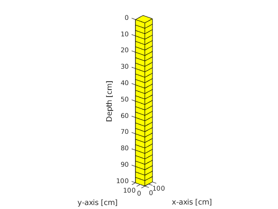
Setting up the Grid¶

nx = 1;               % Cells in x-direction
ny = 1;               % Cells in y-direction
nz = 30;              % Cells in z-direction
Lx = 100;             % Lenght in x-direction
Ly = 100;             % Length in y-direction
Lz = 100;             % Length in z-direction
G = computeGeometry(cartGrid([nx,ny,nz],[Lx,Ly,Lz])); % computing geometry
V = G.cells.volumes;  % Cell volumes

% Plotting Grid
figure(1); plotGrid(G);
xlabel('x-axis [cm]'); ylabel('y-axis [cm]'); zlabel('Depth [cm]');
axis tight; pbaspect([1,1,15]); view([-51,26]);

Fluid Properties¶

rho = 1;                    % [g/cm^3] water density
mu = 0.01;                  % [g/cm.s] water viscosity
g = 980.6650;               % [cm/s^2] gravity acceleration

Rock Properties¶

K_sat = 0.00922;            % [cm/s] saturated hydraulic conductivity
k = (K_sat*mu)/(rho*g);     % [cm^2] intrinsic permeability
rock.perm = repmat([k, k, k], [G.cells.num, 1]); % creating perm structure

Van Genuchten Parameters (Water retention curve)¶

alpha = 0.0335;             % [1/cm] Equation parameter
nVan = 2;                   % [-]    Equation parameter
mVan = 1-(1/nVan);          % [-]    Equation parameter
theta_s = 0.368;            % [-]    Saturation soil moisture
theta_r = 0.102;            % [-]    Residual soil moisture

Boundary and Initial Conditions¶

% Extracting Grid information
zCentr = G.cells.centroids(:,3);   % centroids of cells in z-direction
zFaces = G.faces.centroids(:,3);   % centroids of faces in z-direction
zetaCentr = Lz - zCentr;           % centroids of cells of elev. head
zetaFaces = Lz - zFaces;           % centroids of faces of elev. head

% Determining boundary indices
x_min = find(G.faces.centroids(:,1) == 0);             % west bound indices
x_max = find(G.faces.centroids(:,1) > 0.9999*Lx & ...
             G.faces.centroids(:,1) < 1.0001*Lx );     % east bound indices

y_min = find(G.faces.centroids(:,2) == 0);             % south bound indices
y_max = find(G.faces.centroids(:,2) > 0.9999*Ly & ...
             G.faces.centroids(:,2) < 1.0001*Ly );     % north bound indices

z_min = find(G.faces.centroids(:,3) == 0);             % top bound indices
z_max = find( G.faces.centroids(:,3) > 0.9999*Lz & ...
              G.faces.centroids(:,3) < 1.0001*Lz );    % bottom bound indices

% Boundary values
fluxW = 0;                                  % [cm^3/s] West boundary
fluxE = 0;                                  % [cm^3/s] East boundary
fluxS = 0;                                  % [cm^3/s] South boundary
fluxN = 0;                                  % [cm^3/s] North boundary
psiT = -75;                                 % [cm]     Top boundary
psiB = -1000;                               % [cm]     Bottom boundary

hT = psiT + zetaFaces(z_min);               % [cm] Top hydraulic head
hB = psiB + zetaFaces(z_max);               % [cm] Bottom hydrualic head

% Creating the boundary structure
bc = addBC([], x_min, 'flux', fluxW);       % setting West boundary
bc = addBC(bc, x_max, 'flux', fluxE);       % setting East boundary
bc = addBC(bc, y_min, 'flux', fluxS);       % setting South boundary
bc = addBC(bc, y_max, 'flux', fluxN);       % setting North boundary
bc = addBC(bc, z_min, 'pressure', hT);      % setting Top boundary
bc = addBC(bc, z_max, 'pressure', hB);      % setting Bottom boundary

% Setting the boundary values vector
bc_val = zeros(G.faces.num, 1);             % initializing
bc_val(x_min) = fluxW;                      % assigning West boundary
bc_val(x_max) = fluxE;                      % assigning East boundary
bc_val(y_min) = fluxS;                      % assigning South boundary
bc_val(y_max) = fluxN;                      % assigning North boundary
bc_val(z_min) = hT;                         % assigning Top boundary
bc_val(z_max) = hB;                         % assigning Bottom boundary

% Initial Condition
h_init = psiB + zetaCentr;                  % [cm] Initial condition

Calling MPFA routine¶

mpfa_discr = mpfa(G,rock,[],'bc',bc,'invertBlocks','matlab');

Creating discrete mpfa-operators¶

F = @(x) mpfa_discr.F * x;                  % flux discretization
boundF = @(x) mpfa_discr.boundFlux * x;     % boundary discretization
divF = @(x) mpfa_discr.div * x;             % divergence of the flux

Creating AD variable¶

h_ad = initVariablesADI(h_init);            % Initial value set to h_init

Water retention curves¶

% Boolean function which determines if we are in the unsat or sat zone
isUnsat = @(x) x < 0;

% Water content
theta= @(x)     isUnsat(x) .* ((theta_s - theta_r) ./ ...
                (1 + (alpha .* abs(x)).^nVan).^mVan + theta_r ) + ...
                ~isUnsat(x) .* theta_s;

% Specific Moisture Capacity
C = @(x)        isUnsat(x) .* ((mVan .* nVan .* x .* (theta_r-theta_s) .* ...
                alpha.^nVan .* abs(x).^(nVan-2) ) ./ ...
                (alpha^nVan .* abs(x).^nVan + 1).^(mVan+1)) + ...
                ~isUnsat(x) .* 0;

% Relative permeability
krw= @(x)       isUnsat(x) .* ((1 - (alpha .* abs(x)).^(nVan-1) .* ...
                (1 + (alpha .* abs(x)).^nVan).^(-mVan)).^2 ./ ...
                (1 + (alpha .* abs(x)).^nVan).^(mVan./2)) + ...
                ~isUnsat(x) .* 1;

Time parameters¶

simTime = 72*3600;      % [s]    final simulation time
dt_init = 0.01;         % [s]    initial time step
dt_min = 0.01;          % [s]    minimum time step
dt_max = 10000;         % [s]    maximum time step
lowerOptIterRange = 3;  % [iter] lower optimal iteration range
upperOptIterRange = 7;  % [iter] upper optimal iteration range
lowerMultFactor = 1.3;  % [-]    lower multiplication factor
upperMultFactor = 0.7;  % [-]    upper multiplication factor
dt = dt_init;           % [s]    initializing time step
timeCum = 0;            % [s]    initializing cumulative time
currentTime = 0;        % [s]    current time

Printing parameters¶

printLevels = 10;       % number of printing levels
printTimes = ((simTime/printLevels):(simTime/printLevels):simTime)';
printCounter = 1;       % initializing printing counter
exportCounter = 1;      % intializing exporting counter

Discrete equations¶

% Arithmetic Mean
krwAr = @(h_m0) arithmeticMPFA_hydHead(krw,G,bc,h_m0,zetaCentr,zetaFaces);

% Darcy Flux
q = @(h,h_m0)  (rho.*g./mu) .* krwAr(h_m0) .* (F(h) + boundF(bc_val));

% Mass Conservation
hEq = @(h,h_n0,h_m0,dt) (V./dt) .* (...
                                theta(h_m0-zetaCentr) + ...
                                C(h_m0-zetaCentr) .* (h - h_m0) - ...
                                theta(h_n0-zetaCentr) ...
                                ) + divF(q(h,h_m0));

Creating solution structure¶

sol = struct('time',[],'h',[],'psi',[],'zeta',[],'theta',[],'flux',[],...
             'iter',[],'residual',[],'cpuTime',[]);

% We need to initialize doubles and cells to store the values in sol
t = zeros(printLevels,1);            % Cummulative time
h_cell = cell(printLevels,1);        % Hydraulic Heads
psi_cell = cell(printLevels,1);      % Pressure Heads
zeta_cell = cell(printLevels,1);     % Elevation Heads
theta_cell = cell(printLevels,1);    % Water content
flux_cell = cell(printLevels,1);     % Fluxes
residual = cell(printLevels,1);      % Residuals
iterations = zeros(printLevels,1);   % Iterations
cpuTime = zeros(printLevels,1);      % CPU time

Time loop¶

while timeCum < simTime

    % Newton parameters
    maxTolPresHead = 1; % [cm] maximum absolute tolerance of pressure head
    maxIter = 10;       % maximum number iterations

    % Calling Newton solver
    [h_ad,h_m0,iter,timeCum,tf] = newtonSolver(h_ad,hEq,timeCum,...
                                               dt,maxTolPresHead,maxIter);

    % Calling Time stepping routine
    [dt,printCounter] = timeStepping(dt,dt_min,dt_max,simTime,...
                           timeCum,iter,printTimes,printCounter,...
                           lowerOptIterRange,upperOptIterRange,...
                           lowerMultFactor,upperMultFactor);

    % Storing solutions at each printing time
    if timeCum == printTimes(exportCounter)
        h_cell{exportCounter,1} = h_ad.val;
        psi_cell{exportCounter,1} = h_ad.val - zetaCentr;
        zeta_cell{exportCounter,1} = zetaCentr;
        theta_cell{exportCounter,1} = theta(h_ad.val - zetaCentr);
        flux_cell{exportCounter,1} = q(h_ad.val,h_m0);
        t(exportCounter,1) = timeCum;
        iterations(exportCounter,1) = iter-1;
        cpuTime(exportCounter,1) = tf;
        exportCounter = exportCounter + 1;
    end

end

Time: 0.010 [s]        Iter: 2         Error: 8.659330e-03 [cm]
Time: 0.023 [s]        Iter: 2         Error: 1.436099e-02 [cm]
Time: 0.040 [s]        Iter: 2         Error: 2.368773e-02 [cm]
Time: 0.062 [s]        Iter: 2         Error: 3.880211e-02 [cm]
Time: 0.090 [s]        Iter: 2         Error: 6.300565e-02 [cm]
Time: 0.128 [s]        Iter: 2         Error: 1.011852e-01 [cm]
Time: 0.176 [s]        Iter: 2         Error: 1.602848e-01 [cm]
Time: 0.239 [s]        Iter: 2         Error: 2.496464e-01 [cm]
...

Storing results in the sol structure¶

sol.time = t;           sol.h = h_cell;             sol.psi = psi_cell;
sol.zeta = zeta_cell;   sol.theta = theta_cell;     sol.flux = flux_cell;
sol.iter = iterations;  sol.residual = residual;    sol.cpuTime = cpuTime;

fprintf('\n sol: \n'); disp(sol); % printing solutions in the command window

sol:
        time: [10×1 double]
           h: {10×1 cell}
         psi: {10×1 cell}
        zeta: {10×1 cell}
       theta: {10×1 cell}
        flux: {10×1 cell}
...

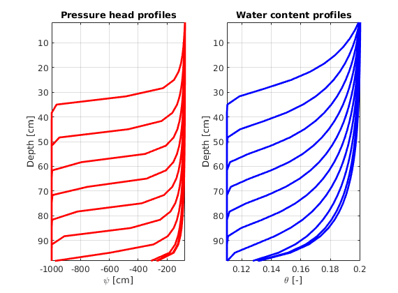
Plotting pressure head and water content profiles¶

figure(2);
for ii=1:printLevels

    subplot(1,2,1); % pressure head plots
    plot(sol.psi{ii,1},G.cells.centroids(:,3),'-r','LineWidth',2)
    t_h1=handle(text('Units','normalized',...
    % Use [%] of the axis length
                     'Position',[0.05,0.95,1],...
% Position of text
                     'EdgeColor','w'));           % Textbox
    t_h1.String=sprintf('Time: %2.1f [hours]',sol.time(ii)/3600);
    ylabel('Depth [cm]'); xlabel('\psi [cm]');
    set(gca,'Ydir','reverse'); axis tight; hold on; box on; grid on;
    title('Pressure head profiles');

    subplot(1,2,2); % water content plots
    plot(sol.theta{ii,1},G.cells.centroids(:,3),'-b','LineWidth',2)
    t_h2=handle(text('Units','normalized',...
    % Use [%] of the axis length
                     'Position',[0.05,0.95,1],...
% Position of text
                     'EdgeColor','w'));           % Textbox
    t_h2.String=sprintf('Time: %2.1f [hours]',sol.time(ii)/3600);
    ylabel('Depth [cm]'); xlabel('\theta [-]');
    set(gca,'Ydir','reverse'); axis tight; hold on; box on; grid on;
    title('Water content profiles');

    pause(1); t_h1.String =[]; t_h2.String =[];
end

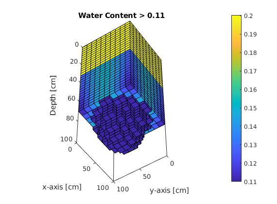
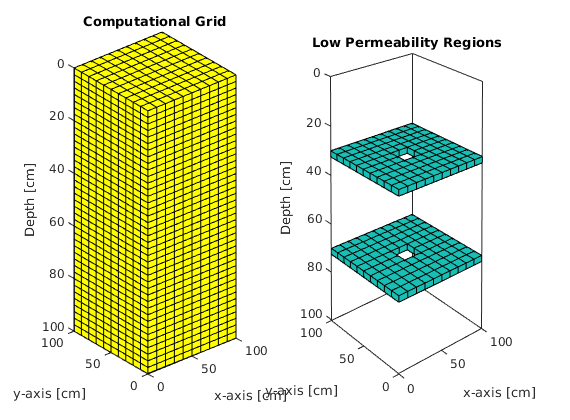
Three-dimensional water infiltration in a heterogeneous domain¶

Generated from waterInfiltration3D.m

This code is an implementation of the mixed-based form of the Richards’ Equation in a three-dimensional domain using Automatic Differentiation from MRST (see http://www.sintef.no/projectweb/mrst/). The grid is set to be cartesian and structured. For the spatial discretization we use cell-centered finite volume method with multi-point flux approximation from https://github.com/keileg/fvbiot. For the time derivative we use the modified picard iteration proposed in: http://onlinelibrary.wiley.com/doi/10.1029/92WR01488/abstract. We decided to use the hydraulic head as primary variable instead of the classical approach (the pressure head) in order to avoid any inconsistency in the gravity contribution. The intrisic permeability at the faces are approximated using harmonic average while the relative permeabilities are upstream weighted. The problem of interest is the vertical infiltration of water (from top to bottom). Moreover, we included low permeability formations near the top and bottom boundaries. For the boundary conditions we use constant

at top and bottom of the domain and no flux elsewhere.

Mass Conservation

$\frac{\partial \theta}{\partial t} + \nabla \cdot \vec{q} = 0$

Multiphase Darcy’s Law

$\vec{q} = -k \frac{\rho g}{\mu} k_{rw} \nabla h$

Mass Conservation

$\frac{V_{\{c\}}}{\Delta t} \left( \theta_{\{c\}}^{n+1,m} + C_{\{c\}}^{n+1,m} \left( h_{\{c\}}^{n+1,m+1} - h_{\{c\}}^{n+1,m} \right) - \theta_{\{c\}}^n \right) + \left[ \mathbf{div} \left( \vec{q}_{\{f\}} \right) \right]_{\{c\}} = 0$

Multiphase Darcy’s Law

$\vec{q}_{\{f\}} = \frac{\rho g}{\mu} \left[ \mathbf{upstr} \left( {k_{rw}}_{\{c\}}^{n+1,m} \right) \right]_{\{f\}} \left( \left[ \mathbf{F} \left( h_{\{c\}}^{n+1,m+1}\right)\right]_{\{f\}} + \left[ \mathbf{boundF} \left(b_{\{f\}} \right) \right]_{\{f\}} \right)$

where

is the soil moisture content,

is the residual moisture content and

,

and

are the van Genuchten’s parameters.

Clearing workspace and cleaning console¶

clear; clc();

Importing modules¶

mrstModule add re-mpfa fvbiot

Setting up the Grid¶

nx = 10;              % Cells in x-direction
ny = 10;              % Cells in y-direction
nz = 40;              % Cells in z-direction
Lx = 100;             % Lenght in x-direction
Ly = 100;             % Length in y-direction
Lz = 100;             % Length in z-direction
G = computeGeometry(cartGrid([nx,ny,nz],[Lx,Ly,Lz])); % computing geometry
V = G.cells.volumes;  % Cell volumes

% Plotting Grid
figure(1); plotGrid(G);
xlabel('x-axis [cm]'); ylabel('y-axis [cm]'); zlabel('Depth [cm]');
axis tight; pbaspect([1,1,4]); view([-51,26]);

Fluid Properties¶

rho = 1;                    % [g/cm^3] water density
mu = 0.01;                  % [g/cm.s] water viscosity
g = 980.6650;               % [cm/s^2] gravity acceleration

Rock Properties¶

K_sat = 0.00922;            % [cm/s] saturated hydraulic conductivity
k = (K_sat*mu)/(rho*g);     % [cm^2] intrinsic permeability
kz = 1E-20 * k;             % [cm^2] low permeability formation
rock.perm = repmat([k, k, k], [G.cells.num, 1]);  % creating perm structure

% Let's add a region of low permeability near the top boundary
rock.perm((12*nx*ny)+1:(12*nx*ny)+(nx*ny),3) = kz;
rock.perm((12*nx*ny)+45:(12*nx*ny)+46,3) = k;
rock.perm((12*nx*ny)+55:(12*nx*ny)+56,3) = k;

% Let's add a region of low permeability near the bottom boundary
rock.perm((28*nx*ny)+1:(28*nx*ny)+(nx*ny),3) = kz;
rock.perm((28*nx*ny)+45:(28*nx*ny)+46,3) = k;
rock.perm((28*nx*ny)+55:(28*nx*ny)+56,3) = k;

Plotting Grid and Low Permeability regions¶

subplot(1,2,1)
   plotGrid(G);
   xlabel('x-axis [cm]'); ylabel('y-axis [cm]'); zlabel('Depth [cm]');
   view([-40 12]); set(gcf,'color','w');
   title('Computational Grid');
subplot(1,2,2)
   plotCellData(G,rock.perm(:,3),rock.perm(:,3) < 1E-20);
   plotGrid(G, 'FaceAlpha', 0, 'EdgeAlpha', .1)
   xlabel('x-axis [cm]'), ylabel('y-axis [cm]'), zlabel('Depth [cm]');
   view([-40 12]); shading faceted; camproj perspective; axis tight;
   set(gca, 'ZDir', 'reverse'); box on;
   title('Low Permeability Regions');

Van Genuchten Parameters¶

alpha = 0.0335;       % [1/cm] Equation parameter
nVan = 2;             % [-]    Equation parameter
mVan = 1-(1/nVan);    % [-]    Equation parameter
theta_s = 0.368;      % [-]    Saturation soil moisture
theta_r = 0.102;      % [-]    Residual soil moisture

Boundary and Initial Conditions¶

% Extracting Grid information
zCentr = G.cells.centroids(:,3);   % centroids of cells in z-direction
zFaces = G.faces.centroids(:,3);   % centroids of faces in z-direction
zetaCentr = Lz - zCentr;           % centroids of cells of elev. head
zetaFaces = Lz - zFaces;           % centroids of faces of elev. head

% Determining boundary indices
x_min = find(G.faces.centroids(:,1) == 0);             % west bound indices
x_max = find(G.faces.centroids(:,1) > 0.9999*Lx & ...
             G.faces.centroids(:,1) < 1.0001*Lx );     % east bound indices

y_min = find(G.faces.centroids(:,2) == 0);             % south bound indices
y_max = find(G.faces.centroids(:,2) > 0.9999*Ly & ...
             G.faces.centroids(:,2) < 1.0001*Ly );     % north bound indices

z_min = find(G.faces.centroids(:,3) == 0);             % top bound indices
z_max = find( G.faces.centroids(:,3) > 0.9999*Lz & ...
              G.faces.centroids(:,3) < 1.0001*Lz );    % bottom bound indices

% Boundary values
fluxW = 0;                                  % [cm^3/s] West boundary
fluxE = 0;                                  % [cm^3/s] East boundary
fluxS = 0;                                  % [cm^3/s] South boundary
fluxN = 0;                                  % [cm^3/s] North boundary
psiT = -75;                                 % [cm]     Top boundary
psiB = -1000;                               % [cm]     Bottom boundary

hT = psiT + zetaFaces(z_min);               % [cm] Top hydraulic head
hB = psiB + zetaFaces(z_max);               % [cm] Bottom hydrualic head

% Creating the boundary structure
bc = addBC([], x_min, 'flux', fluxW);       % setting West boundary
bc = addBC(bc, x_max, 'flux', fluxE);       % setting East boundary
bc = addBC(bc, y_min, 'flux', fluxS);       % setting South boundary
bc = addBC(bc, y_max, 'flux', fluxN);       % setting North boundary
bc = addBC(bc, z_min, 'pressure', hT);      % setting Top boundary
bc = addBC(bc, z_max, 'pressure', hB);      % setting Bottom boundary

% Setting the boundary values vector
bc_val = zeros(G.faces.num, 1);             % initializing
bc_val(x_min) = fluxW;                      % assigning West boundary
bc_val(x_max) = fluxE;                      % assigning East boundary
bc_val(y_min) = fluxS;                      % assigning South boundary
bc_val(y_max) = fluxN;                      % assigning North boundary
bc_val(z_min) = hT;                         % assigning Top boundary
bc_val(z_max) = hB;                         % assigning Bottom boundary

% Initial Condition
h_init = psiB + zetaCentr;                  % [cm] Initial condition

Calling MPFA routine¶

mpfa_discr = mpfa(G,rock,[],'bc',bc,'invertBlocks','matlab');

Creating discrete mpfa-operators¶

F = @(x) mpfa_discr.F * x;                  % flux discretization
boundF = @(x) mpfa_discr.boundFlux * x;     % boundary discretization
divf = @(x) mpfa_discr.div * x;             % divergence

Creating AD variable¶

h_ad = initVariablesADI(h_init);

Water retention curves¶

% Boolean function to determine if we are in the unsat or sat zone
isUnsat = @(x) x < 0;

% Water content
theta= @(x)     isUnsat(x) .* ((theta_s - theta_r) ./ ...
                (1 + (alpha .* abs(x)).^nVan).^mVan + theta_r ) + ...
                ~isUnsat(x) .* theta_s;

% Specific Moisture Capacity
cVan= @(x)      isUnsat(x) .* ((mVan .* nVan .* x .* (theta_r-theta_s) .* ...
                alpha.^nVan .* abs(x).^(nVan-2) ) ./ ...
                (alpha^nVan .* abs(x).^nVan + 1).^(mVan+1)) + ...
                ~isUnsat(x) .* 0;

% Relative permeability
krw= @(x)       isUnsat(x) .* ((1 - (alpha .* abs(x)).^(nVan-1) .* ...
                (1 + (alpha .* abs(x)).^nVan).^(-mVan)).^2 ./ ...
                (1 + (alpha .* abs(x)).^nVan).^(mVan./2)) + ...
                ~isUnsat(x) .* 1;

Time parameters¶

simTime = 96*3600;      % [s]    final simulation time
dt_init = 0.01;         % [s]    initial time step
dt_min = 0.01;          % [s]    minimum time step
dt_max = 10000;         % [s]    maximum time step
lowerOptIterRange = 3;  % [iter] lower optimal iteration range
upperOptIterRange = 7;  % [iter] upper optimal iteration range
lowerMultFactor = 1.3;  % [-]    lower multiplication factor
upperMultFactor = 0.7;  % [-]    upper multiplication factor
dt = dt_init;           % [s]    initializing time step
timeCum = 0;            % [s]    initializing cumulative time
currentTime = 0;        % [s]    current time

Printing parameters¶

printLevels = 20;       % number of printing levels
printTimes = ((simTime/printLevels):(simTime/printLevels):simTime)';   % printing times
printCounter = 1;       % initializing printing counter
exportCounter = 1;      % intializing exporting counter

Discrete equations¶

% Upstream Weighting
krwUp = @(h_m0) upstreamMPFA_hydHead(krw,F,boundF,G,bc,bc_val,h_m0,...
                                     zetaCentr,zetaFaces);

% Darcy Flux
q = @(h,h_m0)  (rho.*g./mu) .* krwUp(h_m0) .* (F(h) + boundF(bc_val));

% Mass Conservation
hEq = @(h,h_n0,h_m0,dt) (V./dt) .* (...
                                theta(h_m0-zetaCentr) + ...
                                cVan(h_m0-zetaCentr) .* (h - h_m0) - ...
                                theta(h_n0-zetaCentr) ...
                                ) + divf(q(h,h_m0));

Creating solution structure¶

sol = struct('time',[],'h',[],'psi',[],'zeta',[],'theta',[],'flux',[],...
             'iter',[],'residual',[],'cpuTime',[]);

% We need to initialize doubles and cells to store the values in sol
t = zeros(printLevels,1);            % Cummulative time
h_cell = cell(printLevels,1);        % Hydraulic Heads
psi_cell = cell(printLevels,1);      % Pressure Heads
zeta_cell = cell(printLevels,1);     % Elevation Heads
theta_cell = cell(printLevels,1);    % Water content
flux_cell = cell(printLevels,1);     % Fluxes
residual = cell(printLevels,1);      % Residuals
iterations = zeros(printLevels,1);   % Iterations
cpuTime = zeros(printLevels,1);      % CPU time

Solving via Newton¶

while timeCum < simTime

    % Newton parameters
    maxTolPresHead = 1; % [cm] maximum absolute tolerance of pressure head
    maxIter = 10;       % maximum number iterations

    % Calling Newton solver
    [h_ad,h_m0,iter,timeCum,tf] = newtonSolver(h_ad,hEq,timeCum,...
                                               dt,maxTolPresHead,maxIter);

    % Calling Time stepping routine
    [dt,printCounter] = timeStepping(dt,dt_min,dt_max,simTime,...
                           timeCum,iter,printTimes,printCounter,...
                           lowerOptIterRange,upperOptIterRange,...
                           lowerMultFactor,upperMultFactor);

    % Storing solutions at each printing time
    if timeCum == printTimes(exportCounter)
        h_cell{exportCounter,1} = h_ad.val;
        psi_cell{exportCounter,1} = h_ad.val - zetaCentr;
        zeta_cell{exportCounter,1} = zetaCentr;
        theta_cell{exportCounter,1} = theta(h_ad.val - zetaCentr);
        flux_cell{exportCounter,1} = q(h_ad.val,h_m0);
        t(exportCounter,1) = timeCum;
        iterations(exportCounter,1) = iter-1;
        cpuTime(exportCounter,1) = tf;
        exportCounter = exportCounter + 1;
    end

end

Time: 0.010 [s]        Iter: 2         Error: 1.059707e-01 [cm]
Time: 0.023 [s]        Iter: 2         Error: 1.677660e-01 [cm]
Time: 0.040 [s]        Iter: 2         Error: 2.611095e-01 [cm]
Time: 0.062 [s]        Iter: 2         Error: 3.980707e-01 [cm]
Time: 0.090 [s]        Iter: 2         Error: 5.920788e-01 [cm]
Time: 0.128 [s]        Iter: 2         Error: 8.555800e-01 [cm]
Time: 0.176 [s]        Iter: 3         Error: 1.606805e-03 [cm]
Time: 0.239 [s]        Iter: 3         Error: 3.031972e-03 [cm]
...

Storing results in the sol structure¶

sol.time = t;           sol.h = h_cell;             sol.psi = psi_cell;
sol.zeta = zeta_cell;   sol.theta = theta_cell;     sol.flux = flux_cell;
sol.iter = iterations;  sol.residual = residual;    sol.cpuTime = cpuTime;

fprintf('\n sol: \n'); disp(sol);  % printing solutions in the command window

sol:
        time: [20×1 double]
           h: {20×1 cell}
         psi: {20×1 cell}
        zeta: {20×1 cell}
       theta: {20×1 cell}
        flux: {20×1 cell}
...

Water content as a function of time¶

figure(3);
for ii=1:printLevels
    plotCellData(G,sol.theta{ii},sol.theta{ii} > theta(-990));
    xlabel('x-axis [cm]'), ylabel('y-axis [cm]'), zlabel('Depth [cm]');
    xlim([0 Lx]); ylim([0 Ly]); zlim([0 Lz]);
    view([-56 -51]); shading faceted; camproj perspective;
    set(gca, 'ZDir', 'reverse'); box on; pbaspect([1 1 2.5]);
    t_h1=handle(text('Units','normalized',...
   % Use [%] of the axis length
                     'Position',[1,0.9,1],...
   % Position of text
                     'EdgeColor','w'));          % Textbox
    t_h1.String=sprintf('Time: %2.2f [h]',sol.time(ii)/3600); % print "time" counter
    title('Water Content > 0.11'); pause(0.5);
    colorbar; caxis([theta(psiB) theta(psiT)]);
    t_h1.String =[];
end

re-mpfa: Richards’ equation with multi-point flux¶

Examples¶

Three-dimensional water evaporation process¶

Clearing workspace and cleaning console¶

Importing modules¶

Setting up the Grid¶

Fluid Properties¶

Rock Properties¶

Van Genuchten Parameters¶

Boundary and Initial Conditions¶

Calling MPFA routine¶

Creating discrete mpfa-operators¶

Creating AD variable¶

Water retention curves¶

Time parameters¶

Printing parameters¶

Discrete equations¶

Creating solution structure¶

Solving via Newton¶

Storing results in the sol structure¶

Cumulative evaporated water and water content reduction¶

Pseudo One-Dimensional water infiltration process¶

Clearing workspace and cleaning console¶

Importing modules¶

Setting up the Grid¶

Fluid Properties¶

Rock Properties¶

Van Genuchten Parameters (Water retention curve)¶

Boundary and Initial Conditions¶

Calling MPFA routine¶

Creating discrete mpfa-operators¶

Creating AD variable¶

Water retention curves¶

Time parameters¶

Printing parameters¶

Discrete equations¶

Creating solution structure¶

Time loop¶

Storing results in the sol structure¶

Plotting pressure head and water content profiles¶

Three-dimensional water infiltration in a heterogeneous domain¶

Clearing workspace and cleaning console¶

Importing modules¶

Setting up the Grid¶

Fluid Properties¶

Rock Properties¶

Plotting Grid and Low Permeability regions¶

Van Genuchten Parameters¶

Boundary and Initial Conditions¶

Calling MPFA routine¶

Creating discrete mpfa-operators¶

Creating AD variable¶

Water retention curves¶

Time parameters¶

Printing parameters¶

Discrete equations¶

Creating solution structure¶

Solving via Newton¶

Storing results in the sol structure¶

Water content as a function of time¶

`re-mpfa`: Richards’ equation with multi-point flux¶