mimetic: Mimetic solvers for pressure problems

Implementation of mimetic finite volume methods for incompressible (Poisson-type) pressure equations. Mimetic finite differences is a class of consistent discretizations that produce cellwise conservative velocity fields. These solvers support the same types of boundary conditions and wells as the incomp module does and can easily be used with the transport solvers contained therein (implicitTransport, explicitTransport).

Contents

Routines supporting the mimetic method for the pressure equation.

Files

computeMimeticIP - Compute mimetic inner product matrices. incompMimetic - Solve incompressible flow problem (fluxes/pressures). solveIncompFlow - Solve incompressible flow problem (fluxes/pressures). [DEPRECATED]

computeMimeticIP(G, rock, varargin)

Compute mimetic inner product matrices.

Synopsis:

S = computeMimeticIP(G, rock)
S = computeMimeticIP(G, rock, 'pn', pv, ...)

Parameters:

• G – Grid structure as described by grid_structure.
• rock –

  Rock data structure with valid field ‘perm’. The permeability is assumed to be in measured in units of metres squared (m^2). Use function ‘darcy’ to convert from (milli)darcies to m^2, e.g.,

  perm = convertFrom(perm, milli*darcy)

  if the permeability is provided in units of millidarcies.

  The field rock.perm may have ONE column for a scalar permeability in each cell, TWO/THREE columns for a diagonal permeability in each cell (in 2/3 D) and THREE/SIX columns for a symmetric full tensor permeability. In the latter case, each cell gets the permeability tensor

  K_i = [ k1 k2 ] in two space dimensions

  [ k2 k3 ]

  K_i = [ k1 k2 k3 ] in three space dimensions

  [ k2 k4 k5 ] [ k3 k5 k6 ]

• 'pn'/pv –

  List of ‘key’/value pairs defining optional parameters. The supported options are:

  • Type – The kind of system to assemble. The choice made

    for this option influences which pressure solvers can be employed later. String. Default value = ‘hybrid’.

    Supported values are:

    • ’hybrid’ : Hybrid system with inverse of B

      (for Schur complement reduction)

    • ’mixed’ : Hybrid system with B

      (for reduction to mixed form)

    • ’tpfa’ : Hybrid system with B

      (for reduction to tpfa form)

    • ’comp_hybrid’ : Both ‘hybrid’ and ‘mixed’

  • InnerProduct – The inner product with which to define

    the mass matrix. String. Default value = ‘ip_simple’.

    Supported values are:

    • ’ip_simple’ : inner product having the 2*tr(K)-term.

    • ’ip_tpf’ : inner product giving method equivalent

      to two-point flux approximation (TPFA).

    • ’ip_quasitpf’ : inner product ‘’close to’’ TPFA

      (equivalent for Cartesian grids with

      diagonal permeability tensor).

    • ’ip_rt’ : Raviart-Thomas for Cartesian grids,

      else not valid.

    • ’ip_quasirt’ :
    • ’ip_qfamily’ :parametric family of inner products.

  • QParam – Extra parameter to inner product family

    qfamily.

  • Verbose – Whether or not to emit progress reports during

    the assembly process. Logical. Default value is dependent upon global MRST setting ‘mrstVerbose’.

  • facetrans If facetrans is specified, the innerproduct is

    modified to account for a face transmissibilities specified as

    [faces, face_transmissibilities]

Returns:

S – Pressure linear system structure having the following fields: - BI / B : inverse of B / B in hybrid/mixed system - type : system type (hybrid or mixed) - ip : inner product name

See also

solveIncompFlow, darcy, permTensor, mrstVerbose.

incompMimetic(state, g, s, fluid, varargin)

Solve incompressible flow problem (fluxes/pressures).

Synopsis:

state = incompMimetic(state, G, S, fluid)
state = incompMimetic(state, G, S, fluid, 'pn1', pv1, ...)

Description:

This function assembles and solves a (block) system of linear equations defining interface fluxes and cell and interface pressures at the next time step in a sequential splitting scheme for the reservoir simulation problem defined by Darcy’s law and a given set of external influences (wells, sources, and boundary conditions).

Parameters:

• state – Reservoir and well solution structure either properly initialized from function ‘initState’, or the results from a previous call to function ‘incompMimetic’ and, possibly, a transport solver such as function ‘explicitTransport’.
• S (G,) – Grid and (mimetic) linear system data structures as defined by function ‘computeMimeticIP’.
• fluid – Fluid data structure as described by ‘fluid_structure’.

Keyword Arguments:  

• W – Well structure as defined by function ‘addWell’. May be empty (i.e., W = []) which is interpreted as a model without any wells.

• bc – Boundary condition structure as defined by function ‘addBC’. This structure accounts for all external boundary conditions to the reservoir flow. May be empty (i.e., bc = []) which is interpreted as all external no-flow (homogeneous Neumann) conditions.

• src – Explicit source contributions as defined by function ‘addSource’. May be empty (i.e., src = []) which is interpreted as a reservoir model without explicit sources.

• rhs – Supply system right-hand side ‘b’ directly. Overrides internally constructed system right-hand side. Must be a three-element cell array, the elements of which are correctly sized for the block system component to be replaced.

  NOTE: This is a special purpose option for use by code which needs to modify the system of linear equations directly, e.g., the ‘adjoint’ code.

• Solver – Which solver mode function ‘incompMimetic’ should employ in assembling and solving the block system of linear equations. String. Default value: Solver = ‘hybrid’.

  Supported values are:

  • ‘hybrid’ –

    Assemble and solve hybrid system for interface pressures. System is eventually solved by Schur complement reduction and back substitution.

    The system ‘S’ must in this case be assembled by passing option pair (‘Type’,’hybrid’) or option pair (‘Type’,’comp_hybrid’) to function ‘computeMimeticIP’.

  • ‘mixed’ –

    Assemble and solve a hybrid system for interface pressures, cell pressures and interface fluxes. System is eventually reduced to a mixed system as per function ‘mixedSymm’.

    The system ‘S’ must in this case be assembled by passing option pair (‘Type’,’mixed’) or option pair (‘Type’,’comp_hybrid’) to function ‘computeMimeticIP’.

  • ‘tpfa’ –

    Assemble and solve a cell-centred system for cell pressures. Interface fluxes recovered through back substitution.

    The system ‘S’ must in this case be assembled by passing option pair (‘Type’,’mixed’) or option pair (‘Type’,’comp_hybrid’) to function ‘computeMimeticIP’.

• LinSolve – Handle to linear system solver software to which the fully assembled system of linear equations will be passed. Assumed to support the syntax

  x = LinSolve(A, b)

  in order to solve a system Ax=b of linear equations. Default value: LinSolve = @mldivide (backslash).

• MatrixOutput – Whether or not to return the final system matrix ‘A’ to the caller of function ‘incompMimetic’. Logical. Default value: MatrixOutput = FALSE.

Returns:

state – Update reservoir and well solution structure with new values for the fields:

• pressure – Pressure values for all cells in the

  discretised reservoir model, ‘G’.

• facePressure –

  Pressure values for all interfaces in the discretised reservoir model, ‘G’.

• flux – Flux across global interfaces corresponding to

  the rows of ‘G.faces.neighbors’.

• A – System matrix. Only returned if specifically

  requested by setting option ‘MatrixOutput’.

• wellSol – Well solution structure array, one element for

  each well in the model, with new values for the fields:

  • flux – Perforation fluxes through all

    perforations for corresponding well. The fluxes are interpreted as injection fluxes, meaning positive values correspond to injection into reservoir while negative values mean production/extraction out of reservoir.

  • pressure – Well bottom-hole pressure.

Note

If there are no external influences, i.e., if all of the structures ‘W’, ‘bc’, and ‘src’ are empty and there are no effects of gravity, and no system right hand side has been supplied externally, then the input state is returned unchanged and a warning is printed in the command window. This warning is printed with message ID

‘incompMimetic:DrivingForce:Missing’

See also

computeMimeticIP, addBC, addSource, addWell, initSimpleFluid initState, solveIncompFlowMS.

solveIncompFlow(varargin)

Solve incompressible flow problem (fluxes/pressures). [DEPRECATED]

Synopsis:

state = solveIncompFlow(state, G, S, fluid)
state = solveIncompFlow(state, G, S, fluid, 'pn1', pv1, ...)

Description:

This function assembles and solves a (block) system of linear equations defining interface fluxes and cell and interface pressures at the next time step in a sequential splitting scheme for the reservoir simulation problem defined by Darcy’s law and a given set of external influences (wells, sources, and boundary conditions).

Parameters:

• state – Reservoir and well solution structure either properly initialized from function ‘initState’, or the results from a previous call to function ‘solveIncompFlow’ and, possibly, a transport solver such as function ‘explicitTransport’.
• S (G,) – Grid and (mimetic) linear system data structures as defined by function ‘computeMimeticIP’.
• fluid – Fluid data structure as described by ‘fluid_structure’.

Keyword Arguments:  

• wells – Well structure as defined by function ‘addWell’. May be empty (i.e., W = []) which is interpreted as a model without any wells.

• bc – Boundary condition structure as defined by function ‘addBC’. This structure accounts for all external boundary conditions to the reservoir flow. May be empty (i.e., bc = []) which is interpreted as all external no-flow (homogeneous Neumann) conditions.

• src – Explicit source contributions as defined by function ‘addSource’. May be empty (i.e., src = []) which is interpreted as a reservoir model without explicit sources.

• rhs – Supply system right-hand side ‘b’ directly. Overrides internally constructed system right-hand side. Must be a three-element cell array, the elements of which are correctly sized for the block system component to be replaced.

  NOTE: This is a special purpose option for use by code which needs to modify the system of linear equations directly, e.g., the ‘adjoint’ code.

• Solver – Which solver mode function ‘solveIncompFlow’ should employ in assembling and solving the block system of linear equations. String. Default value: Solver = ‘hybrid’.

  Supported values are:

  • ‘hybrid’ –

    Assemble and solve hybrid system for interface pressures. System is eventually solved by Schur complement reduction and back substitution.

    The system ‘S’ must in this case be assembled by passing option pair (‘Type’,’hybrid’) or option pair (‘Type’,’comp_hybrid’) to function ‘computeMimeticIP’.

  • ‘mixed’ –

    Assemble and solve a hybrid system for interface pressures, cell pressures and interface fluxes. System is eventually reduced to a mixed system as per function ‘mixedSymm’.

    The system ‘S’ must in this case be assembled by passing option pair (‘Type’,’mixed’) or option pair (‘Type’,’comp_hybrid’) to function ‘computeMimeticIP’.

  • ‘tpfa’ –

    Assemble and solve a cell-centred system for cell pressures. Interface fluxes recovered through back substitution.

    The system ‘S’ must in this case be assembled by passing option pair (‘Type’,’mixed’) or option pair (‘Type’,’comp_hybrid’) to function ‘computeMimeticIP’.

• LinSolve – Handle to linear system solver software to which the fully assembled system of linear equations will be passed. Assumed to support the syntax

  x = LinSolve(A, b)

  in order to solve a system Ax=b of linear equations. Default value: LinSolve = @mldivide (backslash).

• MatrixOutput – Whether or not to return the final system matrix ‘A’ to the caller of function ‘solveIncompFlow’. Logical. Default value: MatrixOutput = FALSE.

Returns:

state – Update reservoir and well solution structure with new values for the fields:

• pressure – Pressure values for all cells in the

  discretised reservoir model, ‘G’.

• facePressure –

  Pressure values for all interfaces in the discretised reservoir model, ‘G’.

• flux – Flux across global interfaces corresponding to

  the rows of ‘G.faces.neighbors’.

• A – System matrix. Only returned if specifically

  requested by setting option ‘MatrixOutput’.

• wellSol – Well solution structure array, one element for

  each well in the model, with new values for the fields:

  • flux – Perforation fluxes through all

    perforations for corresponding well. The fluxes are interpreted as injection fluxes, meaning positive values correspond to injection into reservoir while negative values mean production/extraction out of reservoir.

  • pressure – Well bottom-hole pressure.

Note

This function is deprecated and will be removed in a future release of MRST Please switch to replacement function ‘incompMimetic’.

If there are no external influences, i.e., if all of the structures ‘W’, ‘bc’, and ‘src’ are empty and there are no effects of gravity, and no system right hand side has been supplied externally, then the input state is returned unchanged and a warning is printed in the command window. This warning is printed with message ID

‘incompMimetic:DrivingForce:Missing’

See also

computeMimeticIP, addBC, addSource, addWell, initSimpleFluid initState, solveIncompFlowMS, incompMimetic.

Contents

Files mixedSymm - Solve symmetric system of linear eqns using reduction to a mixed system. schurComplementSymm - Solve symmetric system of linear eqns using Schur Complement analysis. schurComplementSymmFault - Solve symmetric system of linear eqns using Schur Complement analysis. tpfSymm - Solve symmetric system of linear eqns using reduction to two-point system.

mixedSymm(B, C, D, f, g, h, Do, varargin)

Solve symmetric system of linear eqns using reduction to a mixed system.

Synopsis:

[faceFlux, press, lam_n]    = mixedSymm(B, C, D, f, g, h, Do)
[faceFlux, press, lam_n]    = mixedSymm(B, C, D, f, g, h, Do, ...
                                        'pn', pv, ...)
[faceFlux, press, lam_n, A] = mixedSymm(...)

Description:

Solves the symmetric, hybrid (block) system of linear equations

[ B C D ] [ v ] [ f ] [ C’ 0 0 ] [ -p ] = [ g ] [ D’ 0 0 ] [ cp ] [ h ]

with respect to the face flux ‘vf’, the cell pressure ‘p’, and the face (contact) pressure ‘cp’ for Neumann boundary. The system is solved using a reduction to a symmetric mixed system of linear equations

[ Bm Cm Dm ] [ vf ] [ fm ] [ Cm’ 0 0 ] [ -p ] = [ g ] [ Dm’ 0 0 ] [ cp_n ] [ h_n ]

where Bm, Cm are ‘the’ mixed block matrices, and Dm enforces Neumann BCs (size(Dm) = m x mb, where n is the number of faces and mb is the number of boundary faces).

Parameters:

• B – Matrix B in the block system. Assumed SPD.
• C – Block ‘C’ of the block system.
• D – Block ‘D’ of the block system, reduced so as to only apply to the Neumann faces (i.e., external faces for which the pressure is not prescribed).
• f – Block ‘f’ of the block system right hand side.
• g – Block ‘g’ of the block system right hand side.
• h – Block ‘h’ of the block system right hand side, reduced so as to apply only to Neumann faces.
• Do – Matrix mapping face-fluxes to half-face-fluxes.
• 'pn'/pv –

  List of name/value pairs describing options to solver. The following options are supported:

  • ’Regularize’ – TRUE/FALSE, whether or not to enforce

    p(1)==0 (i.e., set pressure zero level). This option may be useful when solving pure Neumann problems.

  • ’MixedB’ – TRUE/FALSE (Default FALSE). Must be set

    to TRUE if input ‘B’ is actually the mixed dicsretization matrix Bm (and not the hybrid). Useful for multiscale when Bm is formed directly.

  • ’LinSolve’ – Function handle to a solver for the

    system above. Assumed to support the syntax

    x = LinSolve(A, b)

    to solve a system Ax=b of linear equations. Default value: LinSolve = @mldivide (backslash).

Returns:

• faceFlux – The face fluxes ‘vf’.
• press – The cell pressure ‘p’.
• lam_n – The contact pressure ‘cp’ on Neumann faces.
• A – Mixed system matrix. OPTIONAL. Only returned if specifically requested.

See also

tpfSymm, schurComplementSymm, solveIncompFlow, solveIncompFlowMS.

schurComplementSymm(BI, C, D, f, g, h, varargin)

Solve symmetric system of linear eqns using Schur Complement analysis.

Synopsis:

[flux, press, lam]    = schurComplementSymm(BI, C, D, f, g, h)
[flux, press, lam]    = schurComplementSymm(BI, C, D, f, g, h, ...
                                            'pn', pv, ...)
[flux, press, lam, S] = schurComplementSymm(...)

Description:

Solves the symmetric, hybrid (block) system of linear equations

[ B C D ] [ v ] [ f ] [ C’ 0 0 ] [ -p ] = [ g ] [ D’ 0 0 ] [ cp ] [ h ]

with respect to the half-face (half-contact) flux ‘v’, the cell pressure ‘p’, and the face (contact) pressure ‘cp’. The system is solved using a Schur complement reduction to a symmetric system of linear equations

S cp = R (*)

from which the contact pressure ‘cp’ is recovered. Then, using back substitution, the cell pressure and half-contact fluxes are recovered.

Note, however, that the function assumes that any faces having prescribed pressure values (such as Dirichlet boundary condtions or wells constrained by BHP targets) have already been eliminated from the blocks ‘D’ and ‘h’.

Parameters:

• BI – Inverse of the matrix B in the block system. Assumed SPD.
• C – Block ‘C’ of the block system.
• D – Block ‘D’ of the block system.
• f – Block ‘f’ of the block system right hand side.
• g – Block ‘g’ of the block system right hand side.
• h – Block ‘h’ of the block system right hand side.
• 'pn'/pv –

  List of ‘key’/value pairs defining optional parameters. The supported options are:

  Regularize – Whether or not to enforce p(1)==0 (i.e., set

  pressure zero level) which may be useful when solving pure Neumann problems. Logicial. Default value = FALSE.

  LinSolve – Function handle to a solver for the system

  (*) above. Assumed to support the syntax

  x = LinSolve(A, b)

  to solve a system Ax=b of linear equations. Default value: LinSolve = @mldivide (backslash).

Returns:

• flux – The half-contact fluxes ‘v’.
• press – The cell pressure ‘p’.
• lam – The contact pressure ‘cp’.
• S – Schur complement reduced system matrix used in recovering contact pressures. OPTIONAL. Only returned if specifically requested.

See also

tpfSymm, mixedSymm, solveIncompFlow, solveIncompFlowMS.

schurComplementSymmFault(BI, C, D, E, f, g, h, varargin)

Solve symmetric system of linear eqns using Schur Complement analysis.

Synopsis:

[flux, press, lam]    = schurComplementSymm(BI, C, D, f, g, h)
[flux, press, lam]    = schurComplementSymm(BI, C, D, f, g, h, ...
                                            'pn', pv, ...)
[flux, press, lam, S] = schurComplementSymm(...)

Description:

Solves the symmetric, hybrid (block) system of linear equations

[ B C D ] [ v ] [ f ] [ C’ 0 0 ] [ -p ] = [ g ] [ D’ 0 E ] [ cp ] [ h ]

with respect to the half-face (half-contact) flux ‘v’, the cell pressure ‘p’, and the face (contact) pressure ‘cp’. The system is solved using a Schur complement reduction to a symmetric system of linear equations

S cp = R (*)

from which the contact pressure ‘cp’ is recovered. Then, using back substitution, the cell pressure and half-contact fluxes are recovered.

Note, however, that the function assumes that any faces having prescribed pressure values (such as Dirichlet boundary condtions or wells constrained by BHP targets) have already been eliminated from the blocks ‘D’ and ‘h’.

Parameters:

• BI – Inverse of the matrix B in the block system. Assumed SPD.
• C – Block ‘C’ of the block system.
• D – Block ‘D’ of the block system.
• f – Block ‘f’ of the block system right hand side.
• g – Block ‘g’ of the block system right hand side.
• h – Block ‘h’ of the block system right hand side.
• 'pn'/pv –

  List of ‘key’/value pairs defining optional parameters. The supported options are:

  Regularize – Whether or not to enforce p(1)==0 (i.e., set

  pressure zero level) which may be useful when solving pure Neumann problems. Logicial. Default value = FALSE.

  LinSolve – Function handle to a solver for the system

  (*) above. Assumed to support the syntax

  x = LinSolve(A, b)

  to solve a system Ax=b of linear equations. Default value: LinSolve = @mldivide (backslash).

Returns:

• flux – The half-contact fluxes ‘v’.
• press – The cell pressure ‘p’.
• lam – The contact pressure ‘cp’.
• S – Schur complement reduced system matrix used in recovering contact pressures. OPTIONAL. Only returned if specifically requested.

See also

tpfSymm, mixedSymm, solveIncompFlow, solveIncompFlowMS.

tpfSymm(B, C, D, f, g, h, Do, varargin)

Solve symmetric system of linear eqns using reduction to two-point system.

Synopsis:

[faceFlux, press, lam_n]    = tpfSymm(B, C, D, f, g, h, Do)
[faceFlux, press, lam_n]    = tpfSymm(B, C, D, f, g, h, Do, ...
                                      'pn', pv, ...)
[faceFlux, press, lam_n, A] = tpfSymm(...)

Description:

Solves the symmetric, hybrid (block) system of linear equations

[ B C D ] [ v ] [ f ] [ C’ 0 0 ] [ -p ] = [ g ] [ D’ 0 0 ] [ cp ] [ h ]

with respect to the face flux ‘vf’, the cell pressure ‘p’, and the face (contact) pressure ‘cp’ for neumann boundary. The system is solved using a reduction to two-point flux system of linear equations

A [p cp_n] = rhs

where A is size m-by-m, m = number of cells + number of Neumann faces. If B is not diagonal, off-diagonal terms are ignored.

Parameters:

• B – Matrix B in the block system. Assumed SPD.
• C – Block ‘C’ of the block system.
• D – Block ‘D’ of the block system, reduced so as to only apply to the Neumann faces (i.e., external faces for which the pressure is not prescribed).
• f – Block ‘f’ of the block system right hand side.
• g – Block ‘g’ of the block system right hand side.
• h – Block ‘h’ of the block system right hand side, reduced so as to apply only to Neumann faces.
• Do – Matrix mapping face-fluxes to half-face-fluxes.
• 'pn'/pv –

  List of name/value pairs describing options to solver. The following options are supported:

  • ’Regularize’ – TRUE/FALSE, whether or not to enforce

    p(1)==0 (i.e., set pressure zero level). This option may be useful when solving pure Neumann problems.

  • ’MixedB’ – TRUE/FALSE (Default FALSE). Must be set

    to TRUE if input ‘B’ is actually the mixed dicsretization matrix Bm (and not the hybrid). Useful for multiscale when Bm is formed directly.

  • ’LinSolve’ – Function handle to a solver for the

    system above. Assumed to support the syntax

    x = LinSolve(A, b)

    to solve a system Ax=b of linear equations. Default value: LinSolve = @mldivide (backslash).

Returns:

• faceFlux – The face fluxes ‘vf’.
• press – The cell pressure ‘p’.
• lam_n – The contact pressure ‘cp’ on Neumann faces.
• A – TPF system matrix. OPTIONAL. Only returned if specifically requested.

See also

mixedSymm, schurComplementSymm, solveIncompFlow, solveIncompFlowMS.

Examples

Basic Mimetic Tutorial

Generated from mimeticExample1.m

The purpose of this example is to give an overview of how to set up and use the single-phase mimetic pressure solver to solve the single-phase pressure equation

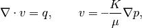
for a flow driven by Dirichlet and Neumann boundary conditions. Our geological model will be simple a Cartesian grid with anisotropic, homogeneous permeability. In this tutorial example, you will learn about:

mrstModule add mimetic incomp

Define geometry

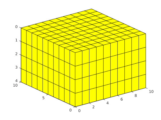
Construct a Cartesian grid of size 10-by-10-by-4 cells, where each cell has dimension 1-by-1-by-1. Because our flow solvers are applicable for general unstructured grids, the Cartesian grid is here represented using an unstructured format, in which cells, faces, nodes, etc. are given explicitly.

nx = 10; ny = 10; nz = 4;
G = cartGrid([nx, ny, nz]);
display(G);

G =

  struct with fields:

       cells: [1×1 struct]
       faces: [1×1 struct]
       nodes: [1×1 struct]
...

After the grid structure is generated, we plot the geometry.

clf, plotGrid(G); view(3),

Process geometry

Having set up the basic structure, we continue to compute centroids and volumes of the cells and centroids, normals, and areas for the faces. For a Cartesian grid, this information can trivially be computed, but is given explicitly so that the flow solver is compatible with fully unstructured grids.

G = computeGeometry(G);

Processing Cells   1 : 400 of 400 ... done (0.02 [s], 2.11e+04 cells/second)
Total 3D Geometry Processing Time = 0.020 [s]

Set rock and fluid data

The only parameters in the single-phase pressure equation are the permeability

and the fluid viscosity

. We set the permeability to be homogeneous and anisotropic

The viscosity is specified by saying that the reservoir is filled with a single fluid, for which de default viscosity value equals unity. Our flow solver is written for a general incompressible flow and requires the evaluation of a total mobility, which is provided by the fluid object.

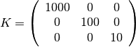
rock.perm = repmat([1000, 100, 10].* milli*darcy(), [G.cells.num, 1]);
fluid     = initSingleFluid('mu' ,    1*centi*poise     , ...
                            'rho', 1014*kilogram/meter^3);

Initialize reservoir simulator

To simplify communication among different flow and transport solvers, all unknowns are collected in a structure. Here this structure is initialized with uniform initial reservoir pressure equal 0 and (single-phase) saturation equal 0.0 (using the default behavior of initResSol)

resSol = initResSol(G, 0.0);
display(resSol);

resSol =

  struct with fields:

    pressure: [400×1 double]
        flux: [1380×1 double]
           s: [400×1 double]

Impose Dirichlet boundary conditions

Our flow solvers automatically assume no-flow conditions on all outer (and inner) boundaries; other type of boundary conditions need to be specified explicitly. Here, we impose Neumann conditions (flux of 1 m^3/day) on the global left-hand side. The fluxes must be given in units of m^3/s, and thus we need to divide by the number of seconds in a day (day()). Similarly, we set Dirichlet boundary conditions p = 0 on the global right-hand side of the grid, respectively. For a single-phase flow, we need not specify the saturation at inflow boundaries. Similarly, fluid composition over outflow faces (here, right) is ignored by pside.

bc = fluxside([], G, 'LEFT',  1*meter^3/day());
bc = pside   (bc, G, 'RIGHT', 0);
display(bc);

bc =

  struct with fields:

     face: [80×1 double]
     type: {1×80 cell}
    value: [80×1 double]
...

Construct linear system

Construct mimetic pressure linear system components for the system Ax = b

based on input grid and rock properties for the case with no gravity.

gravity off;
S = computeMimeticIP(G, rock);

% Plot the structure of the matrix (here we use BI, the inverse of B,
% rather than B because the two have exactly the same structure)
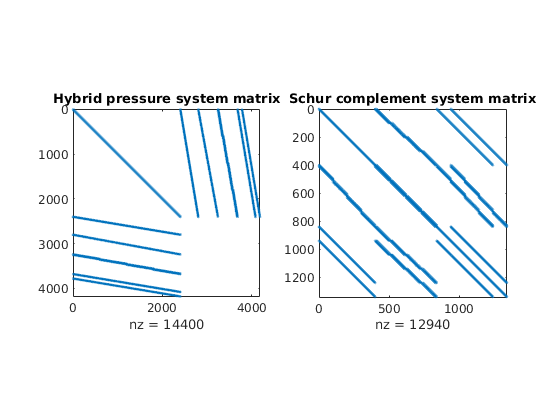
clf, subplot(1,2,1)
cellNo  = rldecode(1:G.cells.num, diff(G.cells.facePos), 2) .';
C       = sparse(1:numel(cellNo), cellNo, 1);
D       = sparse(1:numel(cellNo), double(G.cells.faces(:,1)), 1, ...
                 numel(cellNo), G.faces.num);

spy([S.BI               , C        , D        ; ...
     C', zeros(size(C,2), size(C,2) + size(D,2)); ...
     D', zeros(size(D,2), size(C,2) + size(D,2))]);
title('Hybrid pressure system matrix')

Using inner product: 'ip_simple'.
Computing cell inner products ...             Elapsed time is 0.032099 seconds.
Assembling global inner product matrix ...    Elapsed time is 0.000422 seconds.

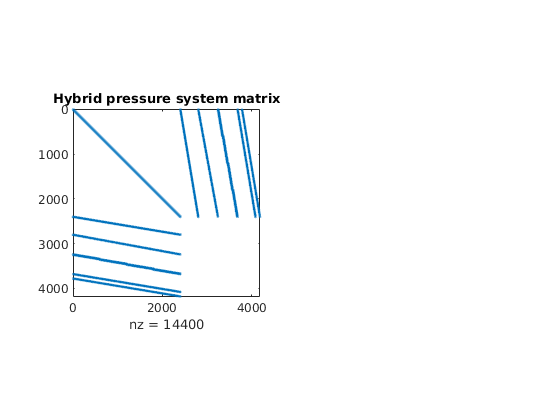
The block structure can clearly be seen in the sparse matrix A, which is never formed in full. Indeed, rather than storing B, we store its inverse B^-1. Similarly, the C and D blocks are not represented in the S structure; they can easily be formed explicitly whenever needed, or their action can easily be computed.

display(S);

S =

  struct with fields:

      BI: [2400×2400 double]
      ip: 'ip_simple'
    type: 'hybrid'

Solve the linear system

Solve linear system construced from S and bc to obtain solution for flow and pressure in the reservoir. The option ‘MatrixOutput=true’ adds the system matrix A to resSol to enable inspection of the matrix.

resSol = incompMimetic(resSol, G, S, fluid, ...
                         'bc', bc, 'MatrixOutput', true);
display(resSol);

resSol =

  struct with fields:

        pressure: [400×1 double]
            flux: [1380×1 double]
               s: [400×1 double]
...

Inspect results

The resSol object contains the Schur complement matrix used to solve the hybrid system.

subplot(1,2,2), spy(resSol.A);
title('Schur complement system matrix');

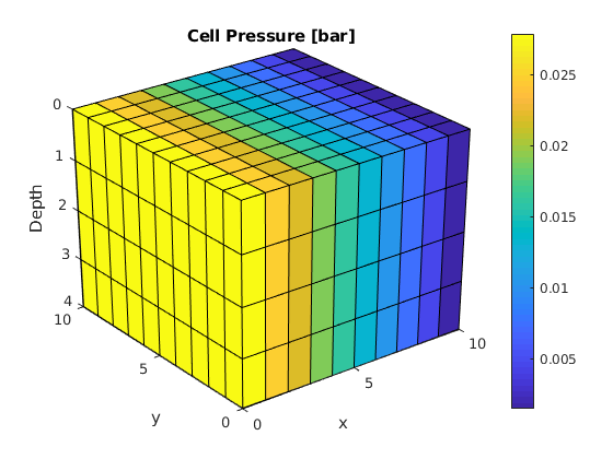
We then plot convert the computed pressure to unit

‘bar’ before plotting result.

clf
plotCellData(G, convertTo(resSol.pressure(1:G.cells.num), barsa()), ...
             'EdgeColor', 'k');
title('Cell Pressure [bar]')
xlabel('x'), ylabel('y'), zlabel('Depth');
view(3); shading faceted; camproj perspective; axis tight;
colorbar

Two-Point Flux Approximation Solvers

Generated from mimeticExample2.m

Use the two-point flux approximation (TPFA) method to solve the single-phase pressure equation

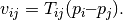
for a Cartesian grid with isotropic, homogeneous permeability and two wells. The problem solved in this example is the same as in the tutorial “Using Peacemann Well Models”, and a more detailed description of the model setup is shown there. The main idea of the TPFA method is to approximate the flux v over a face by the difference of the cell-centered pressures in the neighboring cells weigthed by a face transmissibility T:

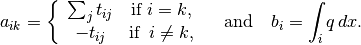
The pressure in each cell is approximated by solving a linear system Ap = b. When ignoring wells, sources, and bc, A and b are given by

Once the pressure is known, the flux is calculated using the expression given above. In this example we show how one can use the mimetic framework to develop a solver that is identical to the classical TPFA solver on Cartesian grids. (However, unlike the TPFA method, the mimetic solver will be consistent also on grids that are not K-orthogonal). The grid and the wells will be the same for both approaches.

mrstModule add mimetic incomp

Define and process geometry

Construct a Cartesian grid of size 10-by-10-by-4 cells, where each cell has dimension 1-by-1-by-1. Because our flow solvers are applicable for general unstructured grids, the Cartesian grid is here represented using an unstructured formate in which cells, faces, nodes, etc. are given explicitly.

nx = 20; ny = 20; nz = 5;
G = cartGrid([nx, ny, nz]);
G = computeGeometry(G, 'Verbose', true);

Processing Cells    1 : 2000 of 2000 ... done (0.02 [s], 1.21e+05 cells/second)
Total 3D Geometry Processing Time = 0.017 [s]

Set rock and fluid data

The only parameters in the single-phase pressure equation are the permeability

, which here is homogeneous, isotropic and equal 100 mD. The fluid has density 1000 kg/m^3 and viscosity 1 cP.

rock.perm = repmat(100 * milli*darcy, [G.cells.num, 1]);
fluid     = initSingleFluid('mu' ,    1*centi*poise     , ...
                            'rho', 1014*kilogram/meter^3);

gravity off

Introduce wells

We will include two wells, one rate-controlled vertical well and one horizontal well controlled by bottom-hole pressure. Wells are described using a Peacemann model, giving an extra set of equations that need to be assembled. We need to specify (‘InnerProduct’, ‘ip_tpf’) to get the correct well model for TPFA. The first well is vertical well (vertical is default):

cellsWell1 =  1 : nx*ny : nx*ny*nz;
radius     = .1;
W = addWell([], G, rock, cellsWell1,          ...
            'Type', 'rate', 'Val', 1.0/day(), ...
            'Radius', radius, 'InnerProduct', 'ip_tpf', 'Comp_i', 1);

cellsWell2 = nx : ny : nx*ny;
W = addWell(W, G, rock, cellsWell2,      ...
            'Type', 'bhp' , 'Val', 1*barsa(), ...
            'Radius', radius, 'Dir', 'y', 'InnerProduct', 'ip_tpf', ...
            'Comp_i', 1);

APPROACH 1: Direct/Classic TPFA

Initialize solution structure with reservoir pressure equal 0. Compute one-sided transmissibilities for each face of the grid from input grid and rock properties. The harmonic averages of ones-sided transmissibilities are computed in the solver incompTPFA.

T = computeTrans(G, rock, 'Verbose', true);

Computing one-sided transmissibilities...     Elapsed time is 0.005090 seconds.

Initialize well solution structure (with correct bhp). No need to assemble well system (wells are added to the linear system inside the incompTPFA-solver).

resSol1 = initState(G, W, 0, 1);

% Solve linear system construced from T and W to obtain solution for flow
% and pressure in the reservoir and the wells. Notice that the TPFA solver
% is different from the one used for mimetic systems.
resSol1 = incompTPFA(resSol1, G, T, fluid, 'wells', W, 'Verbose', true);

Setting up linear system...                   Elapsed time is 0.011004 seconds.
Solving linear system...                      Elapsed time is 0.006908 seconds.
Computing fluxes, face pressures etc...               Elapsed time is 0.002381 seconds.

APPROACH 2: Mimetic with TPFA-inner product

Initialize solution structure with reservoir pressure equal 0. Compute the mimetic inner product from input grid and rock properties.

IP = computeMimeticIP(G, rock, 'Verbose', true, ...
                      'InnerProduct', 'ip_tpf');

Using inner product: 'ip_tpf'.
Computing cell inner products ...             Elapsed time is 0.049135 seconds.
Assembling global inner product matrix ...    Elapsed time is 0.001853 seconds.

Generate the components of the mimetic linear system corresponding to the two wells and initialize the solution structure (with correct bhp)

resSol2 = initState(G, W, 0, 1);

Solve mimetic linear hybrid system

resSol2 = incompMimetic(resSol2, G, IP, fluid, 'wells', W);

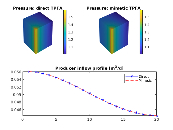
Report results

Report pressure drop computed by the two solvers.

dP1 = convertTo(resSol1.wellSol(1).pressure - ...
                resSol1.wellSol(2).pressure, barsa);
dP2 = convertTo(resSol2.wellSol(1).pressure - ...
                resSol2.wellSol(2).pressure, barsa);
disp(['DeltaP,  direct TPFA: ', num2str(dP1)])
disp(['DeltaP, mimetic TPFA: ', num2str(dP2)])

DeltaP,  direct TPFA: 0.62196
DeltaP, mimetic TPFA: 0.62196

Plot the pressure and producer inflow profile

clf
subplot(2,2,1)
   plotCellData(G, convertTo(resSol1.pressure, barsa),'EdgeColor','none');
   title('Pressure: direct TPFA')
   view(3), camproj perspective, axis tight off, camlight headlight
   colorbar; cax = caxis;

subplot(2,2,2)
   plotCellData(G, convertTo(resSol2.pressure, barsa),'EdgeColor','none');
   title('Pressure: mimetic TPFA')
   view(3), camproj perspective, axis tight off, camlight headlight
   colorbar; caxis(cax);

subplot(2,2,3:4)
   wflux = -[reshape(resSol1.wellSol(2).flux, [], 1), ...
             reshape(resSol2.wellSol(2).flux, [], 1)];
   plot(convertTo(wflux(:,1), meter^3/day), 'b-*'); hold on
   plot(convertTo(wflux(:,2), meter^3/day), 'r--');
   legend('Direct','Mimetic')
   title('Producer inflow profile [m^3/d]');

Copyright notice

<html>
% <p><font size="-1

Two-Point Flux Approximation Solvers with Gravity

Generated from mimeticExample3.m

In this example, we consider a quarter five-spot problem with either wells controlled by pressure or by rate. To compute approximate solutions, we use the two-point flux-approximation scheme formulated in the classical way using transmissibilities and formulated as a mimetic method with a two-point inner product.

mrstModule add mimetic incomp

Define and process geometry

Construct a Cartesian grid of size 10-by-10-by-4 cells, where each cell has dimension 1-by-1-by-1. Because our flow solvers are applicable for general unstructured grids, the Cartesian grid is here represented using an unstructured format in which cells, faces, nodes, etc. are given explicitly.

nx = 20; ny = 20; nz = 20;
G = cartGrid([nx, ny, nz]);
G = computeGeometry(G);

Set rock and fluid data

The only parameters in the single-phase pressure equation are the permeability

, which here is homogeneous, isotropic and equal 100 mD. The fluid has density 1000 kg/m^3 and viscosity 1 cP.

gravity reset on
rock.perm = repmat(100 * milli*darcy, [G.cells.num, 1]);
fluid     = initSingleFluid('mu' ,    1*centi*poise, ...
                            'rho', 1014*kilogram/meter^3);

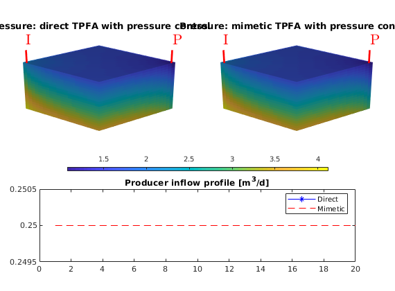
Pressure-controlled wells

We will include two vertical pressure-controlled wells. The wells are described using a Peacemann model, giving an extra set of (trivial) equations that need to be assembled. We need to specify (‘InnerProduct’, ‘ip_tpf’) to get the correct well model for TPFA.

cellsWell1 =  1 : nx*ny : nx*ny*nz;
W = addWell([], G, rock, cellsWell1,          ...
            'Type', 'bhp', 'Val', 2.2049*barsa(), ...
            'InnerProduct', 'ip_tpf', 'Comp_i', 1, 'name', 'I');

cellsWell2 = nx*ny: nx*ny : nx*ny*nz;
W = addWell(W, G, rock, cellsWell2,      ...
            'Type', 'bhp' , 'Val', 1.0*barsa(), ...
            'InnerProduct', 'ip_tpf', 'Comp_i', 1, 'name', 'P');

APPROACH 1: Direct/Classic TPFA Initialize solution structures for reservoir and wells.

resSol1 = initState(G, W, 1.0*barsa, 1);

% Compute one-sided transmissibilities.
T = computeTrans(G, rock, 'Verbose', true);

% Solve linear system construced from T and W to obtain solution for flow
% and pressure in the reservoir and the wells. Notice that the TPFA solver
% is different from the one used for mimetic systems.
resSol1 = incompTPFA(resSol1, G, T, fluid, 'wells', W, 'Verbose', true);

Computing one-sided transmissibilities...     Elapsed time is 0.008366 seconds.
Setting up linear system...                   Elapsed time is 0.018586 seconds.
Solving linear system...                      Elapsed time is 0.042013 seconds.
Computing fluxes, face pressures etc...               Elapsed time is 0.004110 seconds.

APPROACH 2: Mimetic with TPFA-inner product Initialize solution structures for reservoir and wells.

resSol2 = initState(G, W, 0, 1);

% Compute mimetic innerproduct equivalent to two-point flux for Cartesian
% grids.
IP = computeMimeticIP(G, rock, 'Verbose', true, ...
                      'InnerProduct', 'ip_tpf');

%
% Solve mimetic linear hybrid system
resSol2 = incompMimetic(resSol2, G, IP, fluid, 'wells', W);

Using inner product: 'ip_tpf'.
Computing cell inner products ...             Elapsed time is 0.119369 seconds.
Assembling global inner product matrix ...    Elapsed time is 0.004942 seconds.

Report pressure drop computed by the two solvers.

dp = @(x) convertTo(x.wellSol(1).pressure - ...
                    x.wellSol(2).pressure, barsa);

disp(['DeltaP,  direct TPFA: ', num2str(dp(resSol1))])
disp(['DeltaP, mimetic TPFA: ', num2str(dp(resSol2))])

DeltaP,  direct TPFA: 1.2049
DeltaP, mimetic TPFA: 1.2049

Plot the pressure and producer inflow profile

clf
pplot = @(x) plotCellData(G, x, 'EdgeColor','none');
subplot('Position', [0.05,0.55,0.4, 0.35])
   pplot(convertTo(resSol1.pressure(1:G.cells.num), barsa()));
   title('Pressure: direct TPFA with pressure control')
   plotWell(G,W);
   view(45, 25), camproj perspective, axis tight off, camlight headlight
   cax = caxis;

subplot('Position', [0.55,0.55,0.4, 0.35])
   pplot(convertTo(resSol2.pressure(1:G.cells.num), barsa()));
   title('Pressure: mimetic TPFA with pressure control')
   plotWell(G,W);
   view(45, 25), camproj perspective, axis tight off, camlight headlight
   caxis(cax);

subplot('Position', [0.15,0.4,0.7, 0.08])

colorbar south; caxis(cax);axis tight off;

subplot('position', [0.1, 0.1, 0.8, 0.25])
   plot(-convertTo(resSol1.wellSol(2).flux, meter^3/day), 'b-*'); hold on
   plot(-convertTo(resSol2.wellSol(2).flux, meter^3/day), 'r--');
   legend('Direct','Mimetic')
   title('Producer inflow profile [m^3/d]');
   set(gca,'YLim', [.2495 .2505]);

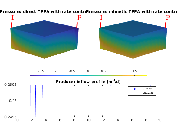
Rate controlled wells

W = addWell([], G, rock, cellsWell1,          ...
            'Type', 'rate', 'Val', 5.0*meter^3/day, ...
            'InnerProduct', 'ip_tpf', 'Comp_i', 1, 'name', 'I');
W = addWell(W, G, rock, cellsWell2,      ...
            'Type', 'rate' , 'Val', -5.0*meter^3/day, ...
            'InnerProduct', 'ip_tpf', 'Comp_i', 1, 'name', 'P');

APPROACH 1: Direct/Classic TPFA

resSol1 = initState(G, W, 0, 1);
resSol1 = incompTPFA(resSol1, G, T, fluid, 'wells', W, 'Verbose', true);

Setting up linear system...                   Elapsed time is 0.016942 seconds.
Solving linear system...                      Elapsed time is 0.031467 seconds.
Computing fluxes, face pressures etc...               Elapsed time is 0.003603 seconds.

APPROACH 2: Mimetic with TPFA-inner product

resSol2 = initState(G, W, 0, 1);
resSol2 = incompMimetic(resSol2, G, IP, fluid, 'wells', W);

Report pressure drop computed by the two solvers.

disp(['DeltaP,  direct TPFA: ', num2str(dp(resSol1))])
disp(['DeltaP, mimetic TPFA: ', num2str(dp(resSol1))])

DeltaP,  direct TPFA: 1.9273
DeltaP, mimetic TPFA: 1.9273

Plot the pressure and producer inflow profile

clf
subplot('Position', [0.05,0.55,0.4, 0.35])
   pplot(convertTo(resSol1.pressure(1:G.cells.num), barsa()));
   title('Pressure: direct TPFA with rate control')
   plotWell(G,W);
   view(45, 25), camproj perspective, axis tight off, camlight headlight
   cax = caxis;

subplot('Position', [0.55,0.55,0.4, 0.35])
   pplot(convertTo(resSol2.pressure(1:G.cells.num), barsa()));
   title('Pressure: mimetic TPFA with rate control')
   plotWell(G,W);
   view(45, 25), camproj perspective, axis tight off, camlight headlight
   caxis(cax);

subplot('Position', [0.15,0.4,0.7, 0.08])

colorbar south; caxis(cax);axis tight off;

subplot('position', [0.1, 0.1, 0.8, 0.25])
   plot(-convertTo(resSol1.wellSol(2).flux, meter^3/day), 'b-*'); hold on
   plot(-convertTo(resSol2.wellSol(2).flux, meter^3/day), 'r--');
   legend('Direct','Mimetic')
   title('Producer inflow profile [m^3/d]');
   set(gca,'YLim', [.2495 .2505]);

Copyright notice

<html>
% <p><font size="-1

Effects of Transmissibility Multipliers

Generated from mimeticExampleSAIGUP.m

Consider once more the incompressible, immiscible two-phase pressure equation

One approach to modelling conduits and barriers to flow is to introduce scalar multipliers on the transmissiblity of a set of grid block connections (cell interfaces). While historically strongly tied to the application of a particular discretisation method (the two-point flux approximation), recent development has demonstrated how to incorporate such multipliers into other consistent and convergent discretisation schemes such as the mimtic method. Here we illustrate effects of transmissibility mulipliers on the qualitative behaviour of the solution of the above problem. Moreover, we demonstrate how the practitioner may introduce multiplier effects in the mimetic method as implemented in MRST.

mrstModule add mimetic incomp deckformat
mrstVerbose false
gravity off

Read input file and construct model

The SAIGUP model is one of the standard data sets provided with MRST. We therefore check if it is present, and if not, download and install it. Then, we read the ECLIPSE input and construct the necessary data objects to make a simulation model

fn = fullfile(getDatasetPath('SAIGUP'),'SAIGUP.GRDECL');
grdecl = readGRDECL(fn);
grdecl = convertInputUnits(grdecl, getUnitSystem('METRIC'));
G      = processGRDECL(grdecl);
G      = computeGeometry(G);
rock   = grdecl2Rock(grdecl, G.cells.indexMap);

Modify the permeability to avoid singular tensors

MRST, or rather the mimetic method implemented in MRST, requires a positive definite permeability tensor in all active grid blocks. The input data of the SAIGUP realisation, however, has zero vertical permeability in a number of cells. We work around this issue by (arbitrarily) assigning the minimum positive vertical (cross-layer) permeability to the grid blocks that have zero cross-layer permeability. We do emphasise that the above restriction does mean that the mimetic method currently implemented in MRST is not capable of handling fully sealing barriers, at least if those barriers are represented as zero grid block permeability.

is_pos = rock.perm(:, 3) > 0;
rock.perm(~is_pos, 3) = min(rock.perm(is_pos, 3));

Extract multipliers from the input data

The computeTranMult function, new in MRST release 2011a, extracts multiplier data from input, typically represented by the ECLIPSE keywords MULTX, MULTY or MULTZ, and computes a scalar multiplier value (default 1.0) for each reservoir connection. The result, m, is represented as a scalar for each face for each grid block, with internal faces being represented twice. In a sense, the computeTranMult function plays a rôle similar to the grdecl2Rock function that extracts and reshapes permeability data from the input model information.

m = computeTranMult(G, grdecl); clear grdecl

Inspect multiplier structure

The multiplier data m is provided once for each face in each grid cell, meaning internal faces are represented twice. However, we need one value per unique face (connection) when we’re plotting this data. Fortunately, the computeTranMult function computes a symmetric assignment, so we need only extract the last multiplier value pertaining to any particular face. This is accomplished by indexing into the (smaller) result array mface with the cell-to-face mapping and then doing regular assignment.

mface = zeros([G.faces.num, 1]);
mface(G.cells.faces(:,1)) = m;

We display the grid structure as a background and add some transparency to the graphics so as not to obscure the multiplier data. Moreover, we only display the multipliers that introduce barriers, i.e., the multipliers that are less than unity. To accentuate the structure of this data, we plot the logarithm of the actual multiplier values.

newplot
[az, el] = deal(-51, 30); daspctrat = [1.2, 2, 1/2];

plotGrid (G, 'EdgeAlpha', 0.05, 'FaceColor', 'none');
plotFaces(G, find(mface < 1), log10(mface(mface < 1)));

view(az, el)
axis tight off, colorbar NorthOutside

set(gca, 'DataAspectRatio', daspctrat);
zoom(1.25)

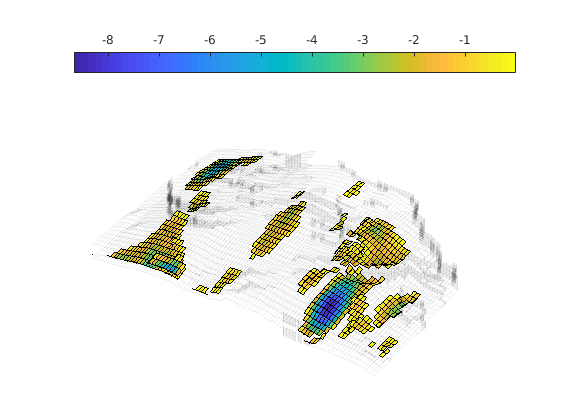
We notice that these multipliers almost exclusively introduce partially sealing flow barriers in the vertical direction. We will additionally introduce lateral flow barriers. The processGRDECL function marks non-neighbouring connections associated with a non-matching corner-point description using a non-zero tag. We first inspect the geometrical structure spanned by these non-neighbouring connections.

newplot
plotGrid (G, 'EdgeAlpha', 0.05, 'FaceColor', 'none');
plotFaces(G, find(abs(G.faces.tag) > 0), ...
          'FaceColor', 'Red', 'EdgeColor', 'none');
view(-126, 40), set(gca, 'DataAspectRatio', daspctrat);
axis tight off
zoom(1.5)

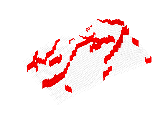
We observe that the fault structures span much of the lateral portion of the model. We will introduce significant flow restriction by assigning a transmissibility multiplier of

to faces associated with any of the faults.

fault_mult = ones([G.faces.num, 1]);
fault_mult(abs(G.faces.tag) > 0) = 5.0e-5;

fault_mult = fault_mult(G.cells.faces(:,1));

Define driving forces

We define a water-flooding scenario in which we inject one 50,000th of the total model pore volume per day in a single injection well. We similarly define a production well controlled by a bottom-hole pressure target of 150 bars.

tot_pv     = sum(poreVolume(G, rock));
inj_rate   = (tot_pv / 50e3) / day;
prod_press = 150*barsa;

We will discretise the pressure equation using both the mimetic and the TPFA method. These methods require different empirical constants in the Peaceman well model, here representeded by the 'InnerProduct' option to the verticalWell well constructor function. First we construct the injection and production wells using the 'ip_quasirt' inner product. This inner product is applicable to the mimetic method we construct below. 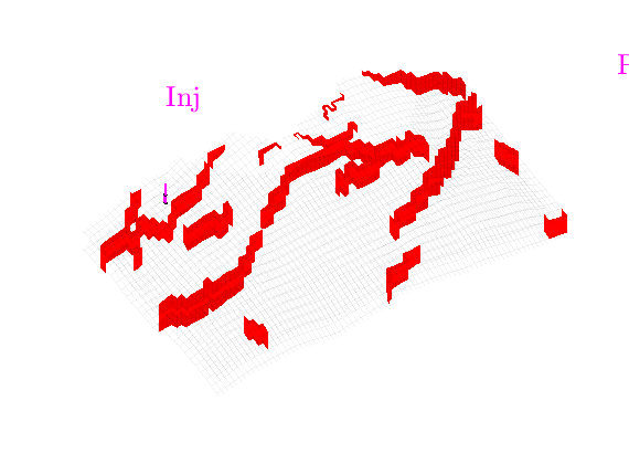We place the injector in an area of the model that is mostly boxed in by the fault structure, so we expect the faults to significantly affect the resulting reservoir flows. Moreover, the producer is in an area that is also mostly shielded from the remainder of the reservoir.

Wm = verticalWell([], G, rock, 30, 85, 1:10       , ...
                 'Type', 'rate', 'Val', inj_rate, ...
                 'Radius', 12.5*centi*meter     , ...
                 'Name', 'Inj'                  , ...
                 'InnerProduct', 'ip_quasirt', 'Comp_i', [1, 0]);

Wm = verticalWell(Wm, G, rock,  5,  12, 1:10       , ...
                 'Type', 'bhp', 'Val', prod_press, ...
                 'Radius', 12.5*centi*meter      , ...
                 'Name', 'Prod'                  , ...
                 'InnerProduct', 'ip_quasirt', 'Comp_i', [0, 1]);

plotWell(G, Wm, 'Height', 200, 'Color', 'magenta', ...
         'cylpts', 30, 'FontSize', 20);

Secondly, we construct the injection and production wells using the 'ip_tpf' inner product. This is Peaceman’s traditional well model that contains the empirical factor 0.14 and is applicable to the two-point discretisation defined below.

Wtp = verticalWell([], G, rock, 30, 85, 1:10   , ...
                   'Type', 'rate', 'Val', inj_rate, ...
                   'Radius', 12.5*centi*meter     , ...
                   'Name', 'Inj'                  , ...
                   'InnerProduct', 'ip_tpf', 'Comp_i', [1, 0]);

Wtp = verticalWell(Wtp, G, rock,  5,  12, 1:10    , ...
                    'Type', 'bhp', 'Val', prod_press, ...
                    'Radius', 12.5*centi*meter      , ...
                    'Name', 'Prod'                  , ...
                    'InnerProduct', 'ip_tpf', 'Comp_i', [0, 1]);

Calculate face transmissibilites

In this problem we consider only barriers to flow. These manifest as transmissibility multipliers less than unity. Selecting multipliers less than

we pick out those multipliers whose effect on the overall solution will be the most distinctive.

An upcoming paper in the SPE Journal shows that multipliers can be incorporated into the mimetic method by computing an associated face transmissibility and subsequently modifying the mimetic inner product using this transmissibility. In particular, if the connection (face) between cells i and j is affected by a multiplier

, then we may add a diagonal contribution of

to the corresponding term in the mimetic inner product in cells i and j, respectively. Here we incorporate the synthetic fault transmissibilities defined above into the actual multiplier data defined in the input, compute the face transmissibilities

(result ftrans) and the multiplier update outlined above (result facetrans). Function computeMimeticIP will then incorporate these values into the pertinent inner products.

m = m .* fault_mult;
i = m < 1e-3;
T = computeTrans(G, rock);

ftrans    = 1 ./ accumarray(G.cells.faces(:,1), 1 ./ T);
facetrans = ftrans(G.cells.faces(i,1)) .* (m(i) ./ (1 - m(i)));

We now calculate the mimetic inner product with and without explicit face transmissibility. Note that we employ the 'ip_quasirt' inner product when constructing the discretisations. This is consistent with the well object defined above.

S0 = computeMimeticIP(G, rock, 'InnerProduct', 'ip_quasirt');
S1 = computeMimeticIP(G, rock, 'InnerProduct', 'ip_quasirt', ...
                      'FaceTrans', ...
                      [G.cells.faces(i,1), facetrans]);

Warning: Matrix is close to singular or badly scaled. Results may be inaccurate.
RCOND =  1.940355e-16.

Create a reservoir fluid

This model problem uses a standard, incompressible fluid with a factor 10 mobility ratio and quadratic relative permeability curves without residual effects.

fluid = initSimpleFluid('mu' , [   1,  10]*centi*poise     , ...
                        'rho', [1000, 700]*kilogram/meter^3, ...
                        'n'  , [   2,   2]);

Initialize the reservoir state object.

The function initState function, new in MRST 2011a, initialises a reservoir- and well solution state object whilst checking its input parameters for basic consistency. In particular, the number of phases must be the same in the well objects and the reservoir state object. We define the reservoir initial condition as a constant pressure of 100 bars and filled with oil (zero water saturation).

xm  = initState(G, Wm   , 100*barsa, [0, 1]);
xtp = initState(G, Wtp, 100*barsa, [0, 1]);

Solve flow problems with and without multiplier effects

Mimetic discretisation without multipliers.

sols{1} = incompMimetic(xm, G, S0, fluid, 'Wells', Wm);

% Mimetic discretisation *with* multipliers.
sols{2} = incompMimetic(xm, G, S1, fluid, 'Wells', Wm);

% Solve the system using TPFA *without* multipliers.
sols{3} = incompTPFA(xtp, G, T, fluid, 'Wells', Wtp);

% Solve the system using TPFA *with* multipliers.
sols{4} = incompTPFA(xtp, G, T .* m, fluid, 'Wells', Wtp);

Warning: Matrix is close to singular or badly scaled. Results may be inaccurate.
RCOND =  1.746419e-17.

Visualise the results

We finally align the pressure results in a 2-by-2 matrix with the results unaffected by multipliers on the left and the multiplier results on the right. The top row is discretised using the mimetic method while the bottom row shows the TPFA results.

clf
ttxt = {'Mimetic without multipliers', 'Mimetic with multipliers', ...
    'TPFA without multipliers', 'TPFA with multipliers'};
for i=1:4
    subplot(2,2,i)
    plotCellData(G, convertTo(sols{i}.pressure, barsa), ...
        'EdgeColor', 'k', 'EdgeAlpha', 0.1)
    view(-80,24), colorbar('horiz'), axis tight off
    set(gca, 'DataAspectRatio', daspctrat), zoom(1.9)
    title(ttxt{i})
end
for i=4:-1:1, subplot(2,2,i), set(gca,'Position',get(gca,'Position')-[0 .1 0 0]); end

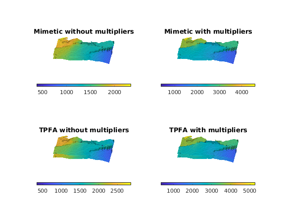
We notice that the results are qualitatively the same between the discretisations (rows), while distinctly different between the models with and without multiplier effects. This demonstrates that it is possible to include barrier modelling in the mimetic method by means of transmissibility multipliers, at least when the multipliers are between zero and one (i.e.,

), and that barrier effects can be quite dramatic.

Copyright notice