book: Book examples
Module containing all the scripts used for the examples, exercises, and figures in the book “An introduction to reservoir simulation using MATLAB” by Knut-Andreas Lie.
Examples
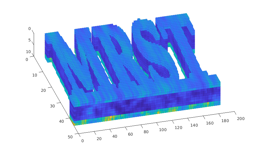
load mrst-logo.mat;
p = .05 + .3*(K(G.cells.indexMap)-30)/600;
rock = makeRock(G, p.^3.*(1e-5)^2./(0.81*72*(1-p).^2), p);
figure('Position',[440 290 860 500]);
plotCellData(G,rock.poro,'EdgeAlpha',.1); view(74,74);
clear p K;
mrstModule add libgeometry incomp;
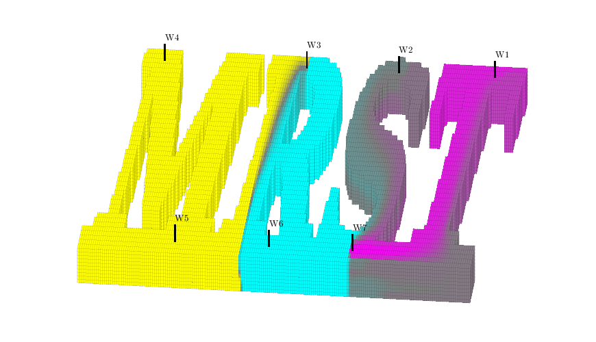
rad = @(x,y) sum(bsxfun(@minus,x(:,1:2),y).^2,2);
G = mcomputeGeometry(G);
pv = sum(poreVolume(G,rock));
W = addWell([],G,rock, find(rad(G.cells.centroids,[3.5,180.5])<0.6), ...
'Type', 'rate','Val', -pv/(20*year));
W = addWell(W,G,rock, find(rad(G.cells.centroids,[3.5,134.5])<0.6), ...
'Type', 'rate','Val', -pv/(20*year));
W = addWell(W,G,rock, find(rad(G.cells.centroids,[3.5,90.5])<0.6), ...
'Type', 'rate','Val', -pv/(20*year));
W = addWell(W,G,rock, find(rad(G.cells.centroids,[3.5,22.5])<0.6), ...
'Type', 'rate','Val', -pv/(20*year));
W = addWell(W,G,rock, find(rad(G.cells.centroids,[42.5,45.5])<0.6), ...
'Type', 'rate','Val', pv/(15*year));
W = addWell(W,G,rock, find(rad(G.cells.centroids,[42.5,90.5])<0.6), ...
'Type', 'rate','Val', pv/(15*year));
W = addWell(W,G,rock, find(rad(G.cells.centroids,[42.5,130.5])<0.6), ...
'Type', 'rate','Val', pv/(15*year));
T = computeTrans(G, rock);
fluid = initSingleFluid('mu' , 1*centi*poise, ...
'rho', 1000*kilogram/meter^3);
state = initState(G,W,100*barsa);
state = incompTPFA(state, G, T, fluid, 'wells', W);
mrstModule add diagnostics
D = computeTOFandTracer(state,G,rock,'wells',W);
figure('Position',[440 290 860 500]);
plotTracerBlend(G, D.ipart, max(D.itracer, [], 2)),
plotWell(G,W,'Color','k','FontSize',10); view(96,76)
plotGrid(G,'EdgeAlpha',.1,'FaceColor','none'); axis off
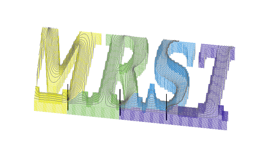
mrstModule add coarsegrid streamlines
cla
p = partitionUI(G,[1 1 G.cartDims(3)]);
plotCellData(G,D.ppart,p>1,'EdgeAlpha',.1,'EdgeColor','k','FaceAlpha',.6);
ip = find( (abs(G.cells.centroids(:,1)-15.5)<.6) & (p==1) & ...
   ((G.cells.centroids(:,2)<35) | (G.cells.centroids(:,2)>65)));
h=streamline(pollock(G,state,ip(1:1:end),'reverse',true));
set(h,'Color',.4*[1 1 1],'LineWidth',.5);
h=streamline(pollock(G,state,ip(1:1:end)));
set(h,'Color',.4*[1 1 1],'LineWidth',.5);
plotWell(G,W,'Color','k','FontSize',0,'height',12,'radius',2);
set(gca,'dataasp',[1.25 2 .4]); zoom(1.2)
Example: specification of boundary conditions
Generated from boundaryConditions.m
In this example, we will show how to set boundary conditions to create pressure drop across a reservoir. For a rectangular model with homogeneous properties, this will create a linear pressure drop. The user can choose between different setups:
mrstModule add incomp

addpath('src');
setup = 3;
Warning: Name is nonexistent or not a directory:
/home/francesca/mrstReleaseCleanRepo/mrst-bitbucket/src
Define geometry
[nx,ny,nz] = deal(20, 20, 5);
[Lx,Ly,Lz] = deal(1000, 1000, 50);
switch setup
   case 1,
      gravity reset off
      G = cartGrid([nx ny nz], [Lx Ly Lz]);
   case 2,
      gravity reset on
      G = cartGrid([nx ny nz], [Lx Ly Lz]);
   case 3,
      gravity reset on
      G = processGRDECL(makeModel3([nx ny nz], [Lx Ly Lz/5]));
      G.nodes.coords(:,3) = 5*(G.nodes.coords(:,3) ...
                               - min(G.nodes.coords(:,3)));
end
G.nodes.coords(:,3) = G.nodes.coords(:,3) + 500;
G = computeGeometry(G);
Adding 800 artificial cells at top/bottom

Processing regular i-faces
 Found 2304 new regular faces
Elapsed time is 0.002980 seconds.

Processing i-faces on faults
 Found 23 faulted stacks
...
Set rock and fluid data
rock.poro = repmat(.2, [G.cells.num, 1]);
rock.perm = repmat([1000, 300, 10].* milli*darcy(), [G.cells.num, 1]);
fluid = initSingleFluid('mu', 1*centi*poise, 'rho', 1014*kilogram/meter^3);
Compute transmissibility and initialize reservoir state
hT = simpleComputeTrans(G, rock);
[mu,rho] = fluid.properties();
state = initResSol(G, G.cells.centroids(:,3)*rho*norm(gravity), 1.0);
Warning:
      4 negative transmissibilities.
      Replaced by absolute values...
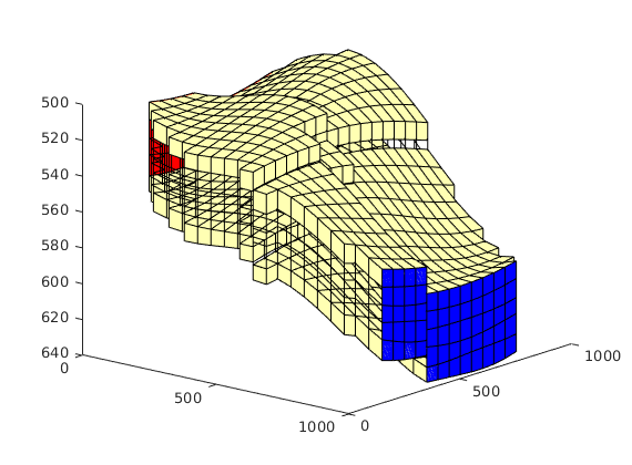
Impose boundary conditions
Our flow solvers automatically assume no-flow conditions on all outer (and inner) boundaries; other type of boundary conditions need to be specified explicitly.
[src,bc] = deal([]);
switch setup
   case 1,
      bc = fluxside(bc, G, 'EAST', 5e3*meter^3/day);
      bc = pside   (bc, G, 'WEST', 50*barsa);

      clf, plotGrid(G,'FaceColor', 'none'); view(3);
      plotFaces(G, bc.face(strcmp(bc.type,'flux')), 'b');
      plotFaces(G, bc.face(strcmp(bc.type,'pressure')), 'r');

   case 2,
      % Alternative 1: use psideh
      % bc = psideh(bc, G, 'EAST', fluid);
      % bc = psideh(bc, G, 'WEST', fluid);
      % bc = psideh(bc, G, 'SOUTH', fluid);
      % bc = psideh(bc, G, 'NORTH', fluid);
      %
      % Alternative 2: compute using face centroids
      % f = boundaryFaces(G);
      % f = f(abs(G.faces.normals(f,3))<eps);
      % bc = addBC(bc,f,'pressure',G.faces.centroids(f,3)*rho*norm(gravity));
      %
      % Alternative 3: sample from initialized state object
      f = boundaryFaces(G);
      f = f(abs(G.faces.normals(f,3))<eps);  % vertical faces only
      cif = sum(G.faces.neighbors(f,:),2);   % cells adjacent to face
      bc = addBC(bc, f, 'pressure', state.pressure(cif));

      clf, plotGrid(G,'FaceColor', 'none'); view(-40,40)
      plotFaces(G, f, state.pressure(cif)/barsa);

      ci = round(.5*(nx*ny-nx));
      ci = [ci; ci+nx*ny];
      src = addSource(src, ci, repmat(-1e3*meter^3/day,numel(ci),1));
      plotGrid(G, ci, 'FaceColor', 'y'); axis tight
      h=colorbar; set(h,'XTick', 1, 'XTickLabel','[bar]');

   case 3,
      clf,
      show = false(nz,1); show([1 nz])=true;
      k = repmat((1:nz),nx*ny,1); k = k(G.cells.indexMap);
      plotGrid(G,'FaceColor','none');
      plotGrid(G, show(k), 'FaceColor', [1 1 .7]);
      view(40,20);

      % First attempt: use pside/fluxside
      bcf = fluxside([], G, 'EAST', 5e3*meter^3/day);
      bcp = pside   ([], G, 'WEST', 50*barsa);
      hf  = plotFaces(G, bcf.face, 'b');
      hp  = plotFaces(G, bcp.face, 'r');

      % Second attempt: count faces
      bcf = fluxside([], G, 'EAST', 5e3*meter^3/day, 4:15, 1:5);
      bcp = pside   ([], G, 'WEST', 50*barsa,        7:17, []);
      delete([hf hp]);
      hf  = plotFaces(G, bcf.face, 'b');
      hp  = plotFaces(G, bcp.face, 'r');

      % Third attempt: do it the hard way
      f = boundaryFaces(G);
      f = f(abs(G.faces.normals(f,3))<eps);  % vertical faces only

      x = G.faces.centroids(f,1);
      [xm,xM] = deal(min(x), max(x));
      ff = f(x>xM-1e-5);
      bc = addBC(bc, ff, 'flux', (5e3*meter^3/day) ...
                 * G.faces.areas(ff)/ sum(G.faces.areas(ff)));
      fp = f(x<xm+1e-5);
      bc = addBC(bc, fp, 'pressure', repmat(50*barsa, numel(fp), 1));

      delete([hf hp]);
      plotFaces(G, ff, 'b'); plotFaces(G, fp, 'r');

end
Solve the linear system and plot result
tate = simpleIncompTPFA(state, G, hT, fluid, 'bc', bc, 'src', src);
clf
plotCellData(G, convertTo(state.pressure, barsa()), 'EdgeColor', 'k');
xlabel('x'), ylabel('y'), zlabel('Depth');
view(3); axis tight;
h=colorbar; set(h,'XTick', 1, 'XTickLabel','[bar]');
Use of Peacemann well models
Generated from firstWellExample.m
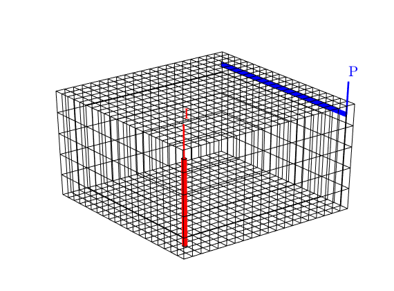
In this example we will demonstrate how to set up a flow problems with two wells, one rate-controlled, vertical well and one horizontal well controlled by bottom-hole pressure. The reservoir is a regular box with homogeneous petrophysical properties.
mrstModule add incomp
Set up reservoir model
[nx,ny,nz] = deal(20,20,5);
G = computeGeometry( cartGrid([nx,ny,nz], [500 500 25]) );
rock  = makeRock(G, 100.*milli*darcy, .2);
fluid = initSingleFluid('mu', 1*centi*poise,'rho', 1014*kilogram/meter^3);
hT    = computeTrans(G, rock);
Add wells wells
W = verticalWell([], G, rock, 1, 1, 1:nz, 'Type', 'rate', 'Comp_i', 1,...
                'Val', 3e3/day, 'Radius', .12*meter, 'name', 'I');
disp('Well #1: '); display(W(1));

W = addWell(W, G, rock, nx : ny : nx*ny, 'Type', 'bhp', 'Comp_i', 1, ...
            'Val', 1.0e5, 'Radius', .12*meter, 'Dir', 'y', 'name', 'P');
disp('Well #2: '); display(W(2));

state = initState(G, W, 0);
Well #1:
        cells: [5×1 double]
         type: 'rate'
          val: 0.0347
            r: [5×1 double]
          dir: [5×1 char]
           rR: [5×1 double]
           WI: [5×1 double]
...
We plot the wells to check if the wells are placed as we wanted them. (The plot will later be moved to subplot(2,2,1), hence we first find the corresponding axes position before generating the handle graphics).
subplot(2,2,1), pos = get(gca,'Position'); clf
plotGrid(G, 'FaceColor', 'none');
view(3), camproj perspective, axis tight off,
plotWell(G, W(1), 'radius',  1, 'height', 5, 'color', 'r');
plotWell(G, W(2), 'radius', .5, 'height', 5, 'color', 'b');
Assemble and solve system
gravity reset on;
state = incompTPFA(state, G, hT, fluid, 'wells', W);
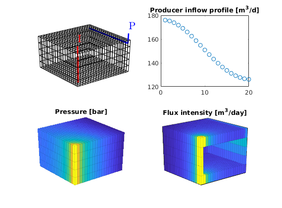
Report results
We move the plot of the grids and wells to the upper-left subplot. The producer inflow profile is shown in the upper-right and the cell pressures in the lower-left subplot. In the lower-right subplot, we show the flux intensity, which must be constructed by averaging over cell faces
subplot(2,2,1)
   set(gca, 'Position', pos);  % move the current plot

subplot(2,2,2)
   plot(convertTo(-state.wellSol(2).flux, meter^3/day),'o')
   title('Producer inflow profile [m^3/d]');

subplot(2,2,3)
   plotCellData(G, convertTo(state.pressure(1:G.cells.num), barsa),'EdgeAlpha',.1);
   title('Pressure [bar]')
   view(3), camproj perspective, axis tight off

subplot(2,2,4)
   [i j k] = ind2sub(G.cartDims, 1:G.cells.num);
   I = false(nx,1); I([1 end])=true;
   J = false(ny,1); J(end)=true;
   K = false(nz,1); K([1 end]) = true;
   cf = accumarray(getCellNoFaces(G), ...
      abs(faceFlux2cellFlux(G, state.flux)));
   plotCellData(G, convertTo(cf, meter^3/day), I(i) | J(j) | K(k),'EdgeAlpha',.1);
   title('Flux intensity [m^3/day]')
   view(-40,20), camproj perspective, axis tight, box on
   set(gca,'XTick',[],'YTick',[],'ZTick',[]);
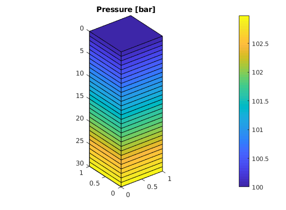
Gravity Column
Generated from gravityColumn.m
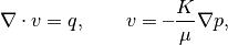
In this example, we introduce a simple pressure solver and use it to solve the single-phase pressure equation
![\nabla\cdot v = q, \qquad
v=\textbf{--}\frac{K}{\mu} \bigl[\nabla p+\rho g\nabla z\bigr],](_images/math/c264092627fac11273b12990e05ce27c1518c064.png)
within the domain [0,1]x[0,1]x[0,30] using a Cartesian grid with homogeneous isotropic permeability of 100 mD. The fluid has density 1000 kg/m^3 and viscosity 1 cP and the pressure is 100 bar at the top of the structure. The purpose of the example is to show the basic steps for setting up, solving, and visualizing a flow problem. More details on the grid structure, the structure used to hold the solutions, and so on, are given in the basic flow-solver tutorial.
addpath('src');
mrstModule add incomp
Warning: Name is nonexistent or not a directory:
/home/francesca/mrstReleaseCleanRepo/mrst-bitbucket/src
Define the model
To set up a model, we need: a grid, rock properties (permeability), a fluid object with density and viscosity, and boundary conditions.
gravity reset on
G     = cartGrid([1, 1, 30], [1, 1, 30]);
G     = computeGeometry(G);
rock  = makeRock(G, 0.1*darcy(), 0.2);
fluid = initSingleFluid('mu' ,    1*centi*poise, ...
                             'rho', 1014*kilogram/meter^3);
bc  = pside([], G, 'TOP', 100.*barsa());
Processing Cells  1 : 30 of 30 ... done (0.00 [s], 1.46e+04 cells/second)
Total 3D Geometry Processing Time = 0.002 [s]
Assemble and solve the linear system
To solve the flow problem, we use the standard two-point flux-approximation method (TPFA), which for a Cartesian grid is the same as a classical seven-point finite-difference scheme for Poisson’s equation. This is done in two steps: first we compute the transmissibilities and then we assemble and solve the corresponding discrete system.
T   = simpleComputeTrans(G, rock);
sol = simpleIncompTPFA(initResSol(G, 0.0), G, T, fluid, 'bc', bc);
Plot the face pressures
ewplot;
plotFaces(G, 1:G.faces.num, convertTo(sol.facePressure, barsa()));
set(gca, 'ZDir', 'reverse'), title('Pressure [bar]')
view(3), colorbar
set(gca,'DataAspect',[1 1 10]);
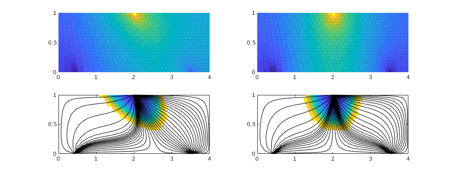
Compare grid-orientation effects for TPFA/mimetic schemes
Generated from gridOrientationError.m
mrstModule add incomp mimetic streamlines diagnostics

% Rectangular reservoir with a skew grid.
G = cartGrid([41,20],[2,1]);
makeSkew = @(c) c(:,1) + .4*(1-(c(:,1)-1).^2).*(1-c(:,2));
G.nodes.coords(:,1) = 2*makeSkew(G.nodes.coords);
% G.nodes.coords = twister(G.nodes.coords);
% G.nodes.coords(:,1) = 2*G.nodes.coords(:,1);
G = computeGeometry(G);

% Homogeneous reservoir properties
rock = makeRock(G, 100*milli*darcy, .2);
pv   = sum(poreVolume(G,rock));

% Symmetric well pattern
srcCells = findEnclosingCell(G,[2 .975; .5 .025; 3.5 .025]);
src = addSource([], srcCells, [pv; -.5*pv; -.5*pv]);

% Single-phase fluid
fluid = initSingleFluid('mu', 1*centi*poise,'rho', 1000*kilogram/meter^3);
Figure and figure settings
figure('Position',[400 460 900 350]);
parg = {'EdgeColor','k','EdgeAlpha',.05};

TPFA solution
hT   = computeTrans(G, rock);
s_tp = initState(G,[], 0);
s_tp = incompTPFA(s_tp, G, hT, fluid, 'src', src);
subplot(2,2,1);
plotCellData(G, s_tp.pressure, 'EdgeColor', 'k', 'EdgeAlpha', .05);
Mimetic solution
S = computeMimeticIP(G, rock);
s_mi = initState(G, [], 0);
s_mi = incompMimetic(s_mi, G, S, fluid, 'src', src);
subplot(2,2,2);
plotCellData(G, s_mi.pressure, 'EdgeColor', 'k', 'EdgeAlpha', .05);
Compare time-of-flight
ubplot(2,2,3);
tof_tp = computeTimeOfFlight(s_tp, G, rock, 'src', src);
plotCellData(G, tof_tp, tof_tp<.2,'EdgeColor','none'); caxis([0 .2]); box on
seed = floor(G.cells.num/5)+(1:G.cartDims(1))';
hf = streamline(pollock(G, s_tp, seed, 'substeps', 1) );
hb = streamline(pollock(G, s_tp, seed, 'substeps', 1, 'reverse' , true));
set ([ hf ; hb ], 'Color' , 'k' );

subplot(2,2,4);
tof_mi = computeTimeOfFlight(s_mi, G, rock, 'src', src);
plotCellData(G, tof_mi, tof_mi<.2,'EdgeColor','none'); caxis([0 .2]); box on
hf = streamline(pollock(G, s_mi, seed, 'substeps', 1) );
hb = streamline(pollock(G, s_mi, seed, 'substeps', 1, 'reverse' , true));
set ([ hf ; hb ], 'Color' , 'k' );
Quarter five spot
Generated from quarterFiveSpot.m
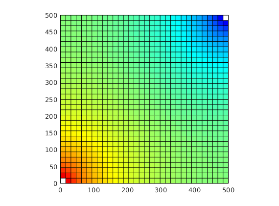
The purpose of this example is to give an overview of how to set up and use the single-phase TPFA pressure solver to solve the pressure equation
with no-flow boundary conditions and two source terms at diagonally opposite corners of a 2D Cartesian grid. This setup mimics a quarter five-spot well pattern, which is a standard test in reservoir simulation. In addition to computing pressure, we will also compute streamlines from the flux field as well as the corresponding time-of-flight, i.e., the time it takes for a neutral particle to travel from a fluid inlet (source term, well, inflow boundary, etc) to a given point in the reservoir.
mrstModule add incomp
Set up grid and petrophysical data
We use a Cartesian grid of size nx-by-ny with homogeneous petrophysical data: permeability of 100 mD and porosity of 0.2.
[nx,ny] = deal(32);
G = cartGrid([nx,ny],[500,500]);
G = computeGeometry(G);
rock = makeRock(G, 100*milli*darcy, .2);
Computing normals, areas, and centroids...    Elapsed time is 0.000321 seconds.
Computing cell volumes and centroids...               Elapsed time is 0.001712 seconds.
Compute half transmissibilities
All we need to know to develop the spatial discretization is the reservoir geometry and the petrophysical properties. This means that we can compute the half transmissibilities without knowing any details about the fluid properties and the boundary conditions and/or sources/sinks that will drive the global flow:
hT = simpleComputeTrans(G, rock);
Fluid model
When gravity forces are absent, the only fluid property we need in the incompressible, single-phase flow equation is the viscosity. However, the flow solver is written for general incompressible flow and requires the evaluation of a fluid object that can be expanded to represent more advanced fluid models. Here, however, we only use a simple fluid object that requires a viscosity and a density (the latter is needed when gravity is present)
gravity reset off
fluid = initSingleFluid('mu' , 1*centi*poise, ...
                        'rho', 1014*kilogram/meter^3);
display(fluid)
fluid =

  struct with fields:

    properties: @(varargin)properties(opt,varargin{:})
    saturation: @(x,varargin)x.s
       relperm: @(s,varargin)relperm(s,opt,varargin{:})
Add source terms
To drive the flow, we will use a fluid source at the SW corner and a fluid sink at the NE corner. The time scale of the problem is defined by the strength of the source term. In our case, we set the source terms such that a unit time corresponds to the injection of one pore volume of fluids. All flow solvers in MRST automatically assume no-flow conditions on all outer (and inner) boundaries if no other conditions are specified explicitly.
pv  = sum(poreVolume(G,rock));
src = addSource([], 1, pv);
src = addSource(src, G.cells.num, -pv);
display(src)
src =

  struct with fields:

    cell: [2×1 double]
    rate: [2×1 double]
     sat: []
Construct reservoir state object
To simplify communication among different flow and transport solvers, all unknowns (reservoir states) are collected in a structure. Strictly speaking, this structure need not be initialized for an incompressible model in which none of the fluid properties depend on the reservoir states. However, to avoid treatment of special cases, MRST requires that the structure is initialized and passed as argument to the pressure solver. We therefore initialize it with a dummy pressure value of zero and a unit fluid saturation since we only have a single fluid
state = initResSol(G, 0.0, 1.0);
display(state)
state =

  struct with fields:

    pressure: [1024×1 double]
        flux: [2112×1 double]
           s: [1024×1 double]
Solve pressure and show the result
To solve for the pressure, we simply pass the reservoir state, grid model, half transsmisibilities, fluid model, and driving forces to the flow solver that assembles and solves the incompressible flow equation.
state = simpleIncompTPFA(state, G, hT, fluid, 'src', src);
display(state)

clf,
plotCellData(G, state.pressure);
plotGrid(G, src.cell, 'FaceColor', 'w');
axis equal tight; colormap(jet(128));
state =

  struct with fields:

        pressure: [1024×1 double]
            flux: [2112×1 double]
               s: [1024×1 double]
...
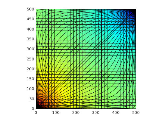
Trace streamlines
To visualize the flow field, we show streamlines. To this end, we will use Pollock’s method which is implemented in the ‘streamlines’ add-on module to MRST. Starting at the midpoint of all cells along the NW–SE diagonal in the grid, we trace streamlines forward and backward using ‘pollock’ and plot them using Matlab’s builtin ‘streamline’ routine
mrstModule add streamlines;
seed = (nx:nx-1:nx*ny).';
Sf = pollock(G, state, seed, 'substeps', 1);
Sb = pollock(G, state, seed, 'substeps', 1, 'reverse', true);
hf=streamline(Sf);
hb=streamline(Sb);
set([hf; hb],'Color','k');
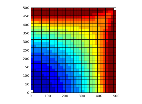
Compute time-of-flight
Finally, we will compute time-of-flight, i.e., the time it takes a neutral particle to travel from the fluid source to a given point in the reservoir. Isocontours of the time-of-flight define natural time lines in the reservoir, and to emphasize this fact, we plot the time-of-flight using only a few colors.
mrstModule add diagnostics
tof = computeTimeOfFlight(state, G, rock, 'src', src);

clf,
plotCellData(G, tof);
plotGrid(G,src.cell,'FaceColor','w');
axis equal tight;
colormap(jet(16)); caxis([0,1]);
Forward maximal TOF set to 0.00 years.
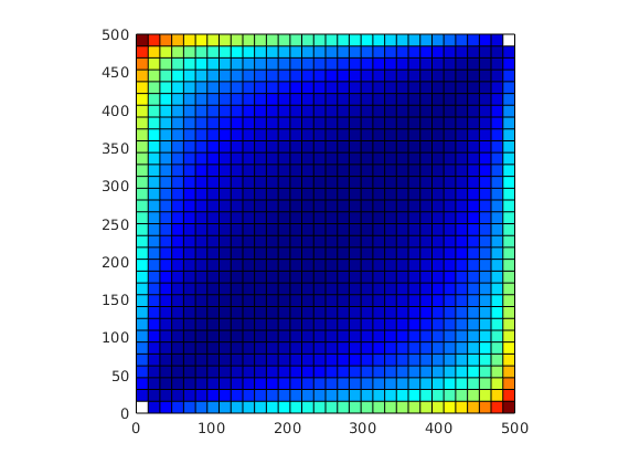
Visualize high-flow and stagnant regions
We can also compute the backward time-of-flight, i.e., the time it takes a neutral particle to travel from a given point in the reservoir to the fluid sink. The sum of the forward and backward time-of-flights give the total travel time in the reservoir, which can be used to visualize high-flow and stagnant regions
tofb   = computeTimeOfFlight(state, G, rock, 'src', src, 'reverse', true);

clf,
plotCellData(G, tof+tofb);
plotGrid(G,src.cell,'FaceColor','w');
axis equal tight;
colormap(jet(128));
Backward maximal TOF set to 0.00 years.
Exercises
Compute a quarter five-spot setup using - perturbed grids, e.g., as computed by ‘twister’ - heterogeneous permeability and porosity, e.g., from a Karman-Cozeny relationship or as subsamples from SPE10
%{
Pressure Solver: Example of a realistic Field Model
Generated from saigupWithWells.m
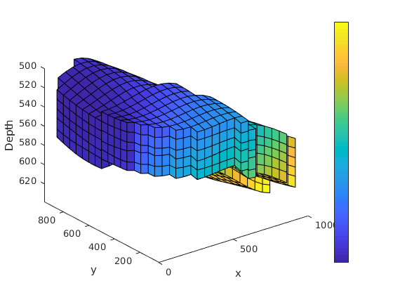
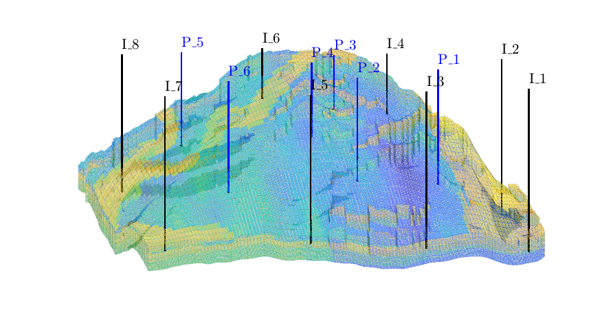
In the example, we will solve the single-phase, incompressible pressure equation using the corner-point geometry from synthetic reservoir model from the SAIGUP study. The purpose of this example is to demonstrate how the two-point flow solver can be applied to compute flow on a real grid model that has degenerate cell geometries and non-neighbouring connections arising from a number of faults, and inactive cells.
Check for existence of input model data
The model can be downloaded from the the MRST page
grdecl = fullfile(getDatasetPath('SAIGUP'), 'SAIGUP.GRDECL');
if ~exist(grdecl, 'file'),
   error('SAIGUP model data is not available.')
end
Load and process grid model
The model data is provided as an ECLIPSE input file. MRST uses the strict SI conventions in all of its internal calculations. The SAIGUP model, however, is provided using the ECLIPSE ‘METRIC’ conventions (permeabilities in mD and so on) and we must therefore convert the input data to MRST’s internal unit conventions.
grdecl = readGRDECL(grdecl);
usys   = getUnitSystem('METRIC');
grdecl = convertInputUnits(grdecl, usys);
G = processGRDECL(grdecl);
G = computeGeometry(G);

% To speed up the processing, one can use a C-accelerated versions of the
% gridprocessing routines (provided you have a compatible compiler):
% mrstModule add libgeometry opm_gridprocessing
% G = mcomputeGeometry(processgrid(grdecl));
Get petrophysical data
The input data of the permeability in the SAIGUP realisation is an anisotropic tensor with zero vertical permeability in a number of cells. As a result some parts of the reservoir to be completely sealed from the wells. This will cause problems for the time-of-flight solver, which requires that all cells in the model must be flooded after some finite time that can be arbitrarily large. We work around this issue by assigning a small constant times the minimum positive vertical (cross-layer) permeability to the grid blocks that have zero cross-layer permeability.
rock = grdecl2Rock(grdecl, G.cells.indexMap);
is_pos = rock.perm(:, 3) > 0;
rock.perm(~is_pos, 3) = 1e-6*min(rock.perm(is_pos, 3));

hT   = computeTrans(G, rock);
Set fluid data
mrstModule add incomp
gravity reset on
fluid = initSingleFluid('mu',1*centi*poise,'rho', 1000*kilogram/meter^3);
Introduce wells
The reservoir is produced using a set of production wells controlled by bottom-hole pressure and rate-controlled injectors. Wells are described using a Peacemann model, giving an extra set of equations that need to be assembled. For simplicity, all wells are assumed to be vertical and are assigned using the logical (i,j) subindex.
% Plot grid outline
figure('position',[440 317 866 480]);
plotCellData(G,log10(rock.perm(:,1)), ...
   'EdgeColor','k','EdgeAlpha',.1,'FaceAlpha',.5);
axis tight off, view(-100,20)

% Set eight vertical injectors around the perimeter of the model, completed
% in each layer.
nz = G.cartDims(3);
I = [ 3, 20,  3, 25,  3, 30,  5, 29];
J = [ 4,  3, 35, 35, 70, 70,113,113];
R = [ 1,  3,  3,  3,  2,  4,  2,  3]*500*meter^3/day;
W = [];
for i = 1 : numel(I),
   W = verticalWell(W, G, rock, I(i), J(i), 1:nz, 'Type', 'rate', ...
      'Val', R(i), 'Radius', .1*meter, 'Comp_i', 1, ...
      'name', ['I$_{', int2str(i), '}$']);
end
plotWell(G, W, 'height', 30, 'color', 'k');
in = numel(W);

% Set six vertical producers, completed in each layer.
I = [15, 12, 25, 21, 29, 12];
J = [25, 51, 51, 60, 95, 90];
for i = 1 : numel(I),
   W = verticalWell(W, G, rock, I(i), J(i), 1:nz, 'Type', 'bhp', ...
      'Val', 200*barsa(), 'Radius', .1*meter, ...
      'name', ['P$_{', int2str(i), '}$'], 'Comp_i',1);
end
plotWell(G,W(in+1:end),'height',30,'color','b');
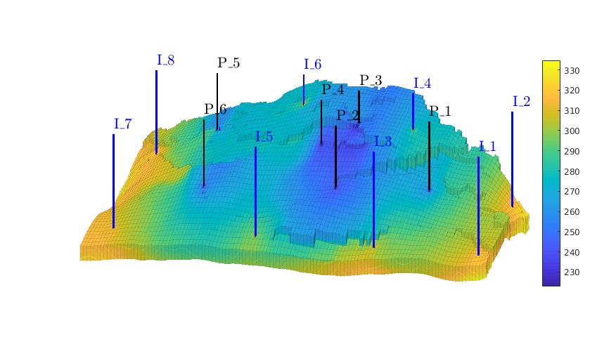
Assemble and solve system, plot results
state = initState(G, W, 350*barsa, 1);
state = incompTPFA(state, G, hT, fluid, 'wells', W);

figure('position',[440 317 866 480]);
plotCellData(G, convertTo(state.pressure(1:G.cells.num), barsa), ...
   'EdgeColor','k','EdgeAlpha',0.1);
plotWell(G, W(1:in),     'height', 100, 'color', 'b');
plotWell(G, W(in+1:end), 'height', 100, 'color', 'k');
axis off; view(-80,36)
h=colorbar; set(h,'Position',[0.88 0.15 0.03 0.67]);
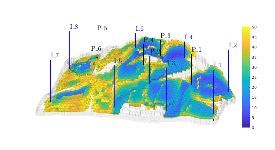
Time-of-flight analysis
rstModule add diagnostics
tf = computeTimeOfFlight(state, G, rock, 'wells', W)/year;
tb = computeTimeOfFlight(state, G, rock, 'wells', W, 'reverse', true)/year;

figure('position',[440 317 866 480]);
plotCellData(G,tf+tb,tf+tb<50,'EdgeColor','k','EdgeAlpha',0.1);
plotWell(G, W(1:in),     'height', 100, 'color', 'b');
plotWell(G, W(in+1:end), 'height', 100, 'color', 'k');
plotGrid(G,'FaceColor','none','edgealpha',.05);
axis off; view(-80,36)
caxis([0 50]);
h=colorbar; set(h,'Position',[0.88 0.15 0.03 0.67]);
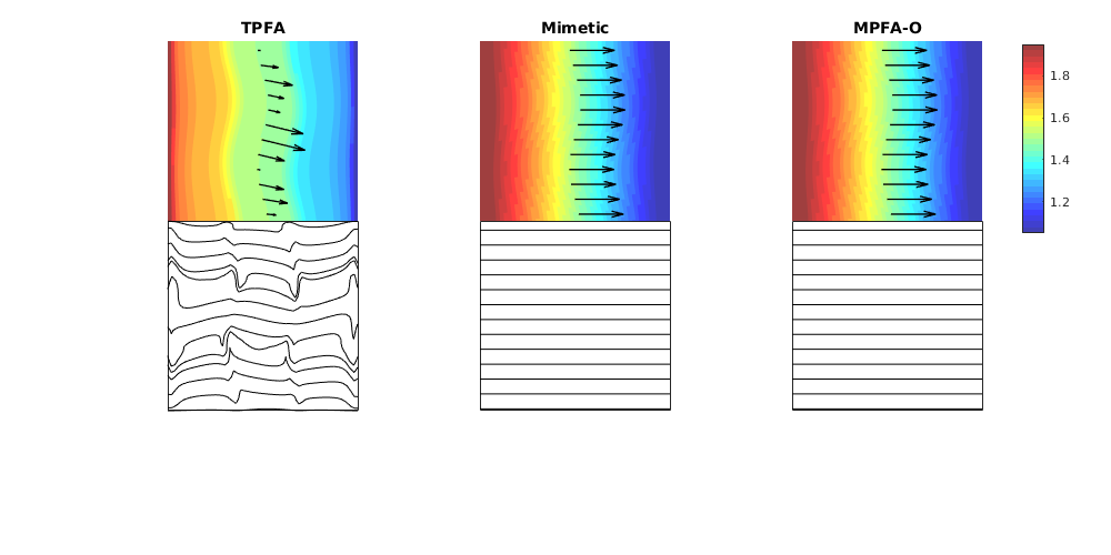
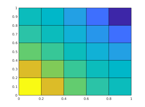
Grid-orientation and anisotropy effects
Generated from showAnisotropyErrors.m
This script contains two examples that originate from the first MRST paper: Lie et al, “Open source MATLAB implementation of consistent discretisations on complex grids”. Comput. Geosci., 16(2):297-322, 2012. DOI: 10.1007/s10596-011-9244-4
addpath(fullfile(fileparts(mfilename('fullpath')), 'src'))
mrstModule add incomp mimetic mpfa
First example
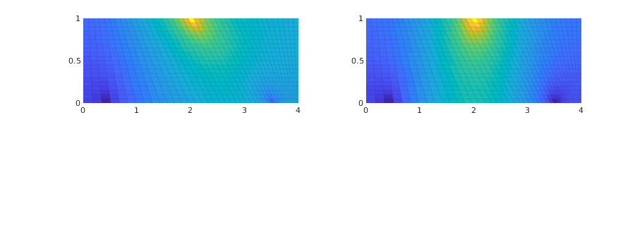
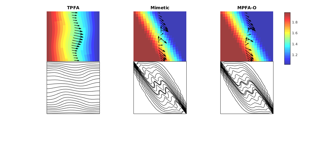
This example corresponds to Figure 7 in the paper, which illustrates grid-orientation effects for the TPFA scheme and reproduction of linear flow for the mimetic and the MPFA-O method on a perturbed grid for a homogeneous, diagonal permeability tensor with entries Kx=1 and Ky=1000.
% Grid and permeability
G = cartGrid([51, 51]);
G.nodes.coords = twister(G.nodes.coords, 0.03);

% Permeability
K = diag([1, 1000]);

% Seed for streamline tracing
seed = (ceil(G.cartDims(1)/2):4*G.cartDims(1):prod(G.cartDims))';

% Run example
showMonotonicityExample(G, K, seed, true);
colormap(.75*jet(32) + .25*ones(32,3));
Computing normals, areas, and centroids...    Elapsed time is 0.000495 seconds.
Computing cell volumes and centroids...               Elapsed time is 0.002857 seconds.
Setting up linear system...                   Elapsed time is 0.029076 seconds.
Solving linear system...                      Elapsed time is 0.003518 seconds.
Computing fluxes, face pressures etc...               Elapsed time is 0.007400 seconds.
Using inner product: 'ip_quasitpf'.
Computing cell inner products ...             Elapsed time is 0.129290 seconds.
Assembling global inner product matrix ...    Elapsed time is 0.000998 seconds.
...
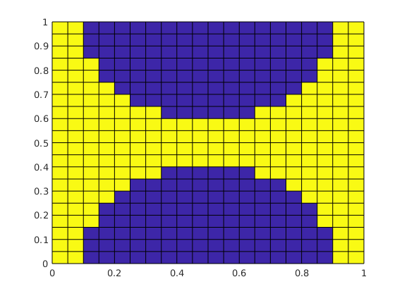
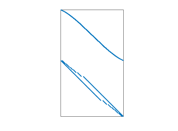
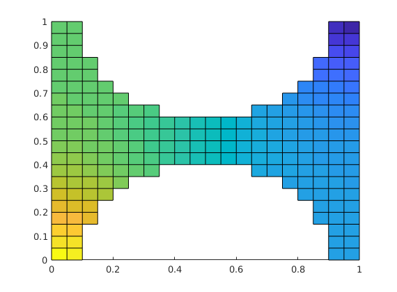
Second example
This example corresponds to Figure 8 in the paper, which illustrates montonicity effects for the TPFA, mimetic, and MPFA schemes. Same setup as in the first example, but now with the anisotropy ration of 1:1000 making 30 degree angle with the grid directions.
% Grid and permeability
G = cartGrid([21, 21]);
G.nodes.coords = twister(G.nodes.coords, 0.03);

% Permeability
t  =  30*pi/180;
U  = [ cos(t), sin(t); -sin(t), cos(t)];
Kd = diag([1,1000]);
K  =  U'*Kd*U;

% Start points for streamline tracing
seed = (ceil(G.cartDims(1)/2):G.cartDims(1):prod(G.cartDims))';

% Run example
showMonotonicityExample(G, K, seed, true);
Computing normals, areas, and centroids...    Elapsed time is 0.000119 seconds.
Computing cell volumes and centroids...               Elapsed time is 0.000869 seconds.
Setting up linear system...                   Elapsed time is 0.002672 seconds.
Solving linear system...                      Elapsed time is 0.000494 seconds.
Computing fluxes, face pressures etc...               Elapsed time is 0.000236 seconds.
Using inner product: 'ip_quasitpf'.
Computing cell inner products ...             Elapsed time is 0.028684 seconds.
Assembling global inner product matrix ...    Elapsed time is 0.001015 seconds.
...
Demonstrate lack of convergence for the TPFA scheme
Generated from showInconsistentTPFA.m
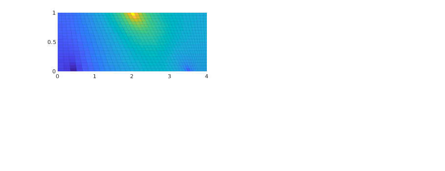
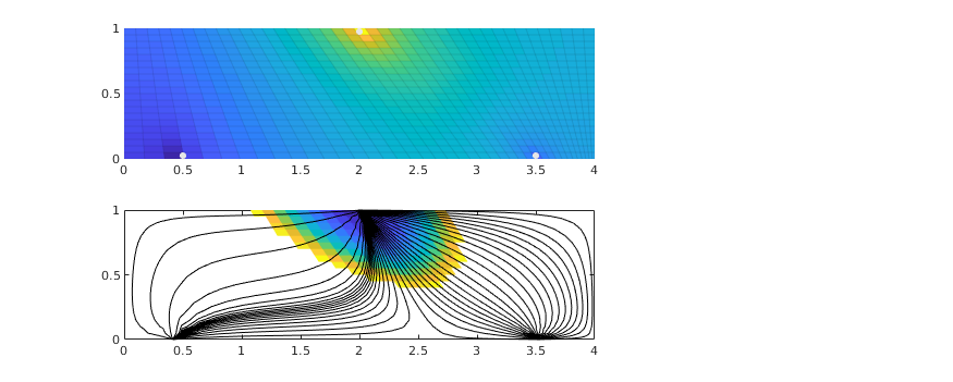
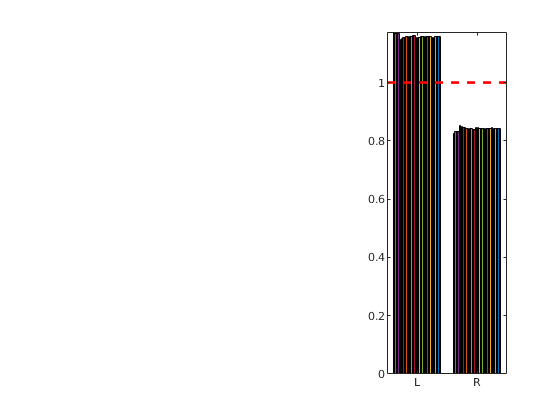
We consider a homogeneous, rectangular reservoir with a symmetric well pattern consisting of one injector and two producers. Because of the symmetry, the travel times from the injector to each producer should be equal. When using a skew grid that is not K-orhtogonal, the travel times will not be equal and the flow pattern will differ quite a lot from being symmetric. In particular, since our discretization method is not consistent, the dissymmetry does not decay with increasing grid resolution and hence the method does not converge.
rstModule add incomp diagnostics streamlines

figure('Position', [440 450 865 351]);
T = nan(30,2);
disp('Convergence study:');
for i=1:1:30
   % Rectangular reservoir with a skew grid.
   G = cartGrid([i*20+1,i*10],[2,1]);
   makeSkew = @(c) c(:,1) + .4*(1-(c(:,1)-1).^2).*(1-c(:,2));
   G.nodes.coords(:,1) = 2*makeSkew(G.nodes.coords);
   G = computeGeometry(G);
   disp(['  Grid: ' num2str(G.cartDims)]);

   % Homogeneous reservoir properties
   rock = makeRock(G, 100*milli*darcy, .2);
   pv   = sum(poreVolume(G,rock));

   % Symmetric well pattern
   srcCells = findEnclosingCell(G,[2 .975; .5 .025; 3.5 .025]);
   src = addSource([], srcCells, [pv; -.5*pv; -.5*pv]);

   % Single-phase fluid
   fluid = initSingleFluid('mu', 1*centi*poise,'rho', 1000*kilogram/meter^3);

   % Solve flow problem
   hT     = computeTrans(G, rock);
   state  = initState(G,[], 0);
   state  = incompTPFA(state, G, hT, fluid, 'src', src);
   tof    = computeTimeOfFlight(state, G, rock, 'src', src);
   T(i,:) = tof(srcCells(2:3))';

   % Plot second solution
   if i==2
      subplot(2,3,1:2);
      plotCellData(G, state.pressure, 'EdgeColor', 'k', 'EdgeAlpha', .05);
      hold on
      plot([.5 2 3.5], [.025 .975 .025],'.','Color',[.9 .9 .9],'MarkerSize',16);
      hold off

      subplot(2,3,4:5);
      plotCellData(G, tof, tof<.2, 'EdgeColor','none'); caxis([0 .2]); box on
      seed = floor(G.cells.num/5)+(1:G.cartDims(1))';
      hf = streamline(pollock(G, state, seed, 'substeps', 1) );
      hb = streamline(pollock(G, state, seed, 'substeps', 1, 'reverse' , true));
      set ([ hf ; hb ], 'Color' , 'k' );
      drawnow;
   end
end
subplot(2,3,[3 6]);
bar(T')
hold on, plot([.5 2.5],[1 1], '--r','LineWidth',2); hold off
set(gca,'XTickLabel', {'L','R'});
axis tight
Convergence study:
  Grid: 21  10
  Grid: 41  20
  Grid: 61  30
  Grid: 81  40
  Grid: 101   50
  Grid: 121   60
  Grid: 141   70
...
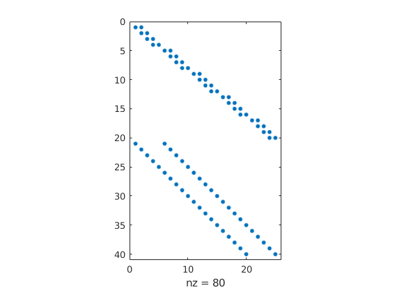
Solve the Poisson problem
Generated from solvePoisson.m
In the first example we use a small Cartesian grid
G = computeGeometry(cartGrid([5 5],[1 1]));
Computing normals, areas, and centroids...    Elapsed time is 0.000135 seconds.
Computing cell volumes and centroids...               Elapsed time is 0.000583 seconds.
Define discrete operators
Since we impose no-flow boundary conditions, we restrict the connections to the interior faces only
N = G.faces.neighbors;
N = N(all(N ~= 0, 2), :);
nf = size(N,1);
nc = G.cells.num;
C = sparse([(1:nf)'; (1:nf)'], N, ones(nf,1)*[-1 1], nf, nc);
grad = @(x) C*x;
div  = @(x) -C'*x;
figure; spy(C);
Set up and solve the problem
p = initVariablesADI(zeros(nc,1));
q = zeros(nc, 1);               % source term
q(1) = 1; q(nc) = -1;           % -> quarter five-spot

eq    = div(grad(p))+q;         % equation
eq(1) = eq(1) + p(1);           % make solution unique
p     = -eq.jac{1}\eq.val;      % solve equation
clf, plotCellData(G, p);
Grid
Generated from solvePoissonCircle.m
G = cartGrid([20 20],[1 1]);
G = computeGeometry(G);
r1 = sum(bsxfun(@minus,G.cells.centroids,[0.5 1]).^2,2);
r2 = sum(bsxfun(@minus,G.cells.centroids,[0.5 0]).^2,2);
clf, plotCellData(G, double((r1>0.16) & (r2>0.16)) );

G = extractSubgrid(G, (r1>0.16) & (r2>0.16));
Computing normals, areas, and centroids...    Elapsed time is 0.000134 seconds.
Computing cell volumes and centroids...               Elapsed time is 0.000813 seconds.
Grid information
N = G.faces.neighbors;
N = N(all(N ~= 0, 2), :);
nf = size(N,1);
nc = G.cells.num;
Operators
C = sparse([(1:nf)'; (1:nf)'], N, ...
    ones(nf,1)*[-1 1], nf, nc);
grad = @(x) C*x;
div  = @(x) -C'*x;
spy(C); set(gca,'XTick',[],'YTick',[]); xlabel([]);
Assemble and solve equations
p = initVariablesADI(zeros(nc,1));
q = zeros(nc, 1);             % source term
q(1) = 1; q(nc) = -1;         % -> quarter five-spot

eq    = div(grad(p))+q;       % equation
eq(1) = eq(1) + p(1);         % make solution unique
p     = -eq.jac{1}\eq.val;    % solve equation
Grid
Generated from solvePoissonSeamount.m
load seamount
G = pebi(triangleGrid([x(:) y(:)], delaunay(x,y)));
G = computeGeometry(G);
clf, plotGrid(G);
axis tight off; set(gca,'XLim',[210.6 211.7]);
Computing normals, areas, and centroids...    Elapsed time is 0.000129 seconds.
Computing cell volumes and centroids...               Elapsed time is 0.000711 seconds.
Grid information
N  = G.faces.neighbors;
N  = N(all(N ~= 0, 2), :);
nf = size(N,1);
nc = G.cells.num;
Operators
C = sparse([(1:nf)'; (1:nf)'], N, ...
    ones(nf,1)*[-1 1], nf, nc);
grad = @(x) C*x;
div  = @(x) -C'*x;
spy(C); set(gca,'XTick',[],'YTick',[]); xlabel([]);

Transmissibility
hT = computeTrans(G, struct('perm', ones(nc,1)));
cf = G.cells.faces(:,1);
T  = 1 ./ accumarray(cf, 1 ./ hT, [G.faces.num, 1]);
T  = T(all(N~=0,2),:);
Assemble and solve equations
p = initVariablesADI(zeros(nc,1));
q = zeros(nc, 1);
q([135 282 17]) = [-1 .5 .5];
eq    = div(T.*grad(p))+q;
eq(1) = eq(1) + p(1);
p     = -eq.jac{1}\eq.val;
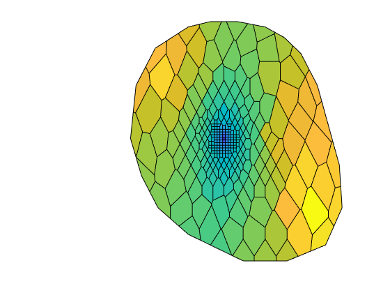
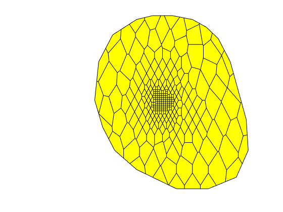
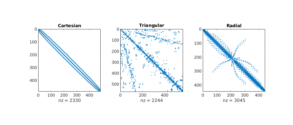
Triangular grid
Generated from stencilComparison.m
load seamount
T = triangleGrid([x(:) y(:)], delaunay(x,y));
[Tmin,Tmax] = deal(min(T.nodes.coords), max(T.nodes.coords));
T.nodes.coords = bsxfun(@times, ...
   bsxfun(@minus, T.nodes.coords, Tmin), 1000./(Tmax - Tmin));
T = computeGeometry(T);
clear x y z Tmin Tmax;
Computing normals, areas, and centroids...    Elapsed time is 0.000162 seconds.
Computing cell volumes and centroids...               Elapsed time is 0.000859 seconds.
Cartesian grids
G = computeGeometry(cartGrid([25 25], [1000 1000]));
inside = isPointInsideGrid(T, G.cells.centroids);
G = removeCells(G, ~inside);

Gr = computeGeometry(cartGrid([250 250], [1000 1000]));
inside = isPointInsideGrid(T, Gr.cells.centroids);
Gr = removeCells(Gr, ~inside);
Computing normals, areas, and centroids...    Elapsed time is 0.000152 seconds.
Computing cell volumes and centroids...               Elapsed time is 0.001048 seconds.
Computing normals, areas, and centroids...    Elapsed time is 0.003370 seconds.
Computing cell volumes and centroids...               Elapsed time is 0.036560 seconds.
Radial grid
P = [];
for r = exp([-3.5:.2:0, 0, .1]),
   [x,y] = cylinder(r,25); P = [P [x(1,:); y(1,:)]]; %#ok<AGROW>
end
P = unique([P'; 0 0],'rows');
[Pmin,Pmax] = deal(min(P), max(P));
P = bsxfun(@minus, bsxfun(@times, ...
   bsxfun(@minus, P, Pmin), 1200./(Pmax-Pmin)), [150 100]);
inside = isPointInsideGrid(T, P);
V = pebi( triangleGrid(P(inside,:)) );
V = computeGeometry(V);
clear P* x y;
Computing normals, areas, and centroids...    Elapsed time is 0.000146 seconds.
Computing cell volumes and centroids...               Elapsed time is 0.000950 seconds.
Simulation loop
mrstModule add incomp diagnostics
state = cell(4,1);
src   = cell(4,1);
bc    = cell(4,1);
A     = cell(4,1);
tof   = cell(4,1);
fluid = initSingleFluid('mu', 1*centi*poise, 'rho', 1014*kilogram/meter^3);
g     = {G, T, V, Gr};
for i=1:4
   rock.poro = repmat(0.2, g{i}.cells.num, 1);
   rock.perm = repmat(100*milli*darcy, g{i}.cells.num, 1);
   hT = simpleComputeTrans(g{i}, rock);
   pv = sum(poreVolume(g{i}, rock));

   tmp = (g{i}.cells.centroids - repmat([450, 500],g{i}.cells.num,1)).^2;
   [~,ind] = min(sum(tmp,2));
   src{i} = addSource(src{i}, ind, -.02*pv/year);

   f = boundaryFaces(g{i});
   bc{i} = addBC([], f, 'pressure', 50*barsa);

   state{i} = incompTPFA(initResSol(g{i},0,1), ...
      g{i}, hT, fluid, 'src', src{i}, 'bc', bc{i}, 'MatrixOutput', true);

   [tof{i},A{i}] = computeTimeOfFlight(state{i}, g{i}, rock,...
      'src', src{i},'bc',bc{i}, 'reverse', true);
end
Setting up linear system...                   Elapsed time is 0.003491 seconds.
Solving linear system...                      Elapsed time is 0.000790 seconds.
Computing fluxes, face pressures etc...               Elapsed time is 0.000249 seconds.
Backward maximal TOF set to 2500.00 years.
Setting up linear system...                   Elapsed time is 0.001687 seconds.
Solving linear system...                      Elapsed time is 0.000618 seconds.
Computing fluxes, face pressures etc...               Elapsed time is 0.000210 seconds.
Backward maximal TOF set to 2500.00 years.
...
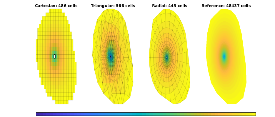
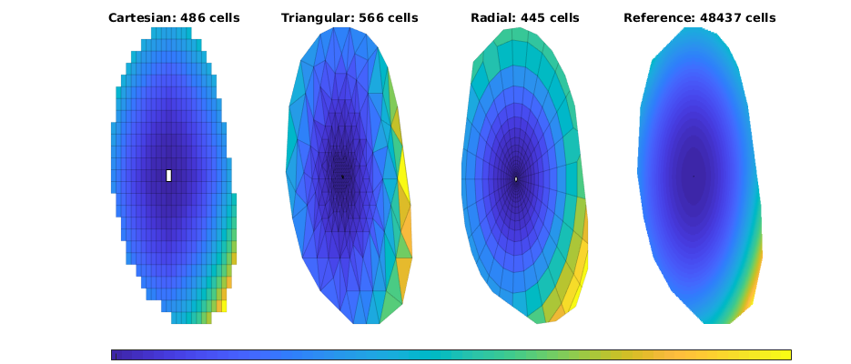
Plot solutions
figure(1), clf, set(gcf,'Position', [400 420 925 400]);
ttext = {'Cartesian','Triangular','Radial','Reference'};
for i=1:4
   subplot(1,4,i),
   plotCellData(g{i},state{i}.pressure/barsa,'EdgeColor','k', 'EdgeAlpha', .1);
   plotGrid(g{i},src{i}.cell, 'FaceColor', 'w');
   title([ttext{i} ': ' num2str(g{i}.cells.num) ' cells']);
   caxis([40 50]); axis tight off
end
set(get(gca,'Children'),'EdgeColor','none');
h=colorbar('Location','South');
set(h,'position',[0.13 0.01 0.8 0.03],'YTick',1,'YTickLabel','[bar]');
set(gcf,'PaperPositionMode', 'auto');
% print -dpng stencil-p.png;
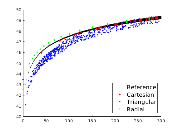
Plot radial solutions
col = 'rbgk';
ms  = [12 8 8 2];
figure(2), clf, hold on
for i=[4 1:3]
  d = g{i}.cells.centroids - repmat(g{i}.cells.centroids(src{i}.cell,:),g{i}.cells.num,1);
  r = (sum(d.^2,2)).^.5;
  plot(r, state{i}.pressure/barsa, [col(i) '.'],'MarkerSize',ms(i));
end
axis([0 300 40 50]);
h=legend(ttext{[4 1:3]},'Location','SouthEast'); set(h,'FontSize',14);
chld = get(h,'Children');
set(chld(1:3:end),'MarkerSize',20);
% print -depsc2 stencil-rad.eps;
Plot matrix structures: TPFA matrix
figure(3); clf, set(gcf,'Position', [400 420 925 400]);
for i=1:3
   subplot(1,3,i),
   spy(state{i}.A);
   title(ttext{i});
end
set(gcf,'PaperPositionMode', 'auto');
% print -depsc2 stencil-A.eps;
Plot solutions
figure(4), clf, set(gcf,'Position', [400 420 925 400]);
ttext = {'Cartesian','Triangular','Radial','Reference'};
for i=1:4
   subplot(1,4,i),
   plotCellData(g{i},tof{i}/year,'EdgeColor','k', 'EdgeAlpha', .1);
   plotGrid(g{i},src{i}.cell, 'FaceColor', 'w');
   title([ttext{i} ': ' num2str(g{i}.cells.num) ' cells']);
   axis tight off
end
set(get(gca,'Children'),'EdgeColor','none');
h=colorbar('Location','South');
set(h,'position',[0.13 0.01 0.8 0.03],'YTick',1,'YTickLabel','[year]');
set(gcf,'PaperPositionMode', 'auto');
% print -dpng stencil-tof.png;
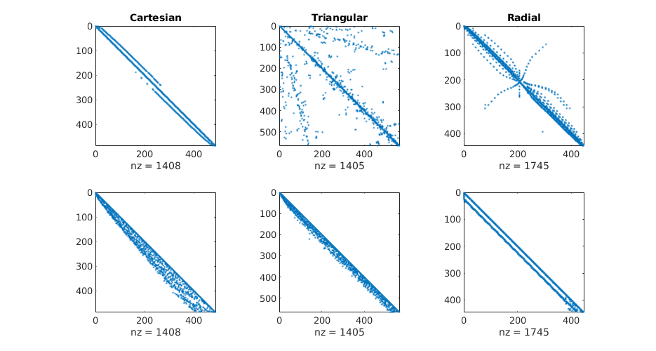
Plot matrix structures: TPFA matrix
igure(5); clf, set(gcf,'Position', [400 420 925 500]);
for i=1:3
   subplot(2,3,i),
   spy(A{i});
   title(ttext{i});
   subplot(2,3,i+3)
   [~,q] = sort(state{i}.pressure);
   spy(A{i}(q,q));
   l = triu(A{i}(q,q),1);
   if sum(l(:))
      disp(['Discretization matrix: ' ttext{i} ', *not* lower triangular']);
   else
      disp(['Discretization matrix: ' ttext{i} ', lower triangular']);
   end
end
set(gcf,'PaperPositionMode', 'auto');
% print -depsc2 stencil-A-tof.eps;
Discretization matrix: Cartesian, lower triangular
Discretization matrix: Triangular, lower triangular
Discretization matrix: Radial, lower triangular
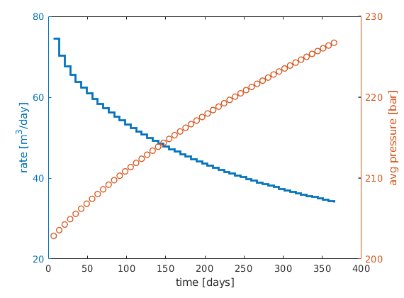
Non-Newtonian fluid
Generated from nonNewtonianCell.m
In this example, we will demonstrate how one can easily extend the compressible single-phase pressure solver to include the effect of non-Newtonian fluids modelled using a simple power law in which the effective viscosity depends on the norm of the velocity
Define geometric quantitites
Grid that represents the reservoir geometry
[nx,ny,nz] = deal( 10,  10, 10);
[Lx,Ly,Lz] = deal(200, 200, 50);
G = cartGrid([nx, ny, nz], [Lx, Ly, Lz]);
G = computeGeometry(G);

% Discrete operators
N  = double(G.faces.neighbors);
intInx = all(N ~= 0, 2);
N  = N(intInx, :);
n = size(N,1);
C = sparse( [(1:n)'; (1:n)'], N, ones(n,1)*[-1 1], n, G.cells.num);
aC = bsxfun(@rdivide,0.5*abs(C),G.faces.areas(intInx))';
grad = @(x) C*x;
div  = @(x) -C'*x;
cavg = @(x) aC*x;
favg = @(x) 0.5 * (x(N(:,1)) + x(N(:,2)));
clear aC C N;
Rock model and transmissibilities
rock = makeRock(G, 30*milli*darcy, 0.3);

cr   = 1e-6/barsa;
p_r  = 200*barsa;
pv_r = poreVolume(G, rock);
pv   = @(p) pv_r .* exp( cr * (p - p_r) );
clear pv_r;

hT = computeTrans(G, rock);
cf = G.cells.faces(:,1);
nf = G.faces.num;
T  = 1 ./ accumarray(cf, 1 ./ hT, [nf, 1]);
T  = T(intInx);
clear hT;
Basic fluid model
c     = 1e-3/barsa;
rho_r = 850*kilogram/meter^3;
rhoS  = 750*kilogram/meter^3;
rho   = @(p) rho_r .* exp( c * (p - p_r) );
if exist('fluidModel', 'var')
   mu0 = fluidModel.mu0;
   nmu = fluidModel.nmu;
   Kc  = fluidModel.Kc;
   Kbc = (Kc/mu0)^(2/(nmu-1))*36*((3*nmu+1)/(4*nmu))^(2*nmu/(nmu-1));
   if nmu==1, Kbc = 0; end
else
   mu0 = 100*centi*poise;
   nmu = 0.25;
   Kc  = .1;
   Kbc = (Kc/mu0)^(2/(nmu-1))*36*((3*nmu+1)/(4*nmu))^(2*nmu/(nmu-1));
end
Initial vertical equilibrium
gravity reset on, g = norm(gravity);
[z_0, z_max] = deal(0, max(G.cells.centroids(:,3)));
equil  = ode23(@(z,p) g .* rho(p), [z_0, z_max], p_r);
p_init = reshape(deval(equil, G.cells.centroids(:,3)), [], 1);
clear equil z_0 z_max;
Constant for the simulation
numSteps = 52;
totTime  = 365*day;
dt       = totTime / numSteps;
tol      = 1e-5;
maxits   = 100;
Flow equations
phiK  = rock.perm.*rock.poro;
gradz = grad(G.cells.centroids(:,3));
v     = @(p, eta) ...
        -(T./(mu0*favg(eta))).*( grad(p) - g*favg(rho(p)).*gradz );
etaEq = @(p, eta) ...
        eta - ( 1 + Kbc* cavg(v(p,eta)).^2 ./phiK ).^((nmu-1)/2);
presEq= @(p, p0, eta, dt)  ...
        (1/dt)*(pv(p).*rho(p) - pv(p0).*rho(p0)) + div(favg(rho(p)).*v(p, eta));
Well model
nperf = 8;
I = repmat(2, [nperf, 1]);
J = (1 : nperf).' + 1;
K = repmat(5, [nperf, 1]);
cellInx = sub2ind(G.cartDims, I, J, K);
W = addWell([ ], G, rock, cellInx, 'Name', 'P1', 'Dir', 'x' );

% Define well equations
wc = W(1).cells; % connection grid cells
WI = W(1).WI;    % well-indices
dz = W(1).dZ;    % connection depth relative to bottom-hole

p_conn = @(bhp) ...
   bhp + g*dz.*rho(bhp);
q_conn = @(p, eta, bhp) ...
   WI .* (rho(p(wc)) ./ (mu0*eta(wc))) .* (p_conn(bhp) - p(wc));
rateEq = @(p, eta, bhp, qS) ...
   qS - sum(q_conn(p, eta, bhp))/rhoS;
ctrlEq = @(bhp) ...
   bhp - 300*barsa;
Initialize for solution loop
nc = G.cells.num;
[p_ad, eta_ad, bhp_ad, qS_ad] = ...
   initVariablesADI(p_init, ones(nc,1), p_init(wc(1)), 0);
[pIx, etaIx, bhpIx, qSIx] = ...
   deal(1:nc, nc+1:2*nc, 2*nc+1, 2*nc+2);
sol = repmat(struct('time',[],'pressure',[],'eta',[], ...
                    'bhp',[],'qS',[]), [numSteps+1,1]);
sol(1) = struct('time', 0, 'pressure', value(p_ad), ...
                'eta', value(eta_ad), ...
                'bhp', value(bhp_ad), 'qS', value(qS_ad));
[etamin, etawmin, etamean] = deal(zeros(numSteps,1));
Time loop
t = 0; step = 0;
while t < totTime

   % Increment time
   t = t + dt;
   step = step + 1;
   fprintf('Time step %d: Time %.2f -> %.2f days\n', ...
      step, convertTo(t - dt, day), convertTo(t, day));

   % Main Newton loop
   p0  = value(p_ad); % Previous step pressure
   [resNorm,nit] = deal(1e99, 0);
   while (resNorm > tol) && (nit < maxits)

      % Newton loop for eta (effective viscosity)
      [resNorm2,nit2] = deal(1e99, 0);
      eta_ad2 = initVariablesADI(eta_ad.val);
      while (resNorm2 > tol) && (nit2 <= maxits)
         eeq = etaEq(p_ad.val, eta_ad2);
         res = eeq.val;
         eta_ad2.val = eta_ad2.val - (eeq.jac{1} \ res);

         resNorm2 = norm(res);
         nit2     = nit2+1;
      end
      if nit2 > maxits
         error('Local Newton solves did not converge')
      else
         eta_ad.val = eta_ad2.val;
      end

      % Add source terms to homogeneous pressure equation:
      eq1     = presEq(p_ad, p0, eta_ad, dt);
      eq1(wc) = eq1(wc) - q_conn(p_ad, eta_ad, bhp_ad);

      % Collect all equations
      eqs = {eq1, etaEq(p_ad, eta_ad), ...
         rateEq(p_ad, eta_ad, bhp_ad, qS_ad), ctrlEq(bhp_ad)};

      % Concatenate equations and solve for update:
      eq  = cat(eqs{:});
      J   = eq.jac{1};  % Jacobian
      res = eq.val;     % residual
      upd = -(J \ res); % Newton update
      % Update variables
      p_ad.val   = p_ad.val   + upd(pIx);
      eta_ad.val = eta_ad.val + upd(etaIx);
      bhp_ad.val = bhp_ad.val + upd(bhpIx);
      qS_ad.val  = qS_ad.val  + upd(qSIx);

      resNorm = norm(res);
      nit     = nit + 1;
   end

 %  clf,
 %  plotCellData(G,eta_ad.val,'FaceAlpha',.3,'EdgeAlpha', .1);
 %  view(3); colorbar; drawnow

   if nit > maxits
      error('Newton solves did not converge')
   else % store solution
      sol(step+1)  = struct('time', t, 'pressure', value(p_ad), ...
         'eta', value(eta_ad), ...
         'bhp', value(bhp_ad), 'qS', value(qS_ad));
   end
   etamin (step) = min(eta_ad.val);
   etawmin(step) = min(eta_ad.val(wc));
   etamean(step) = mean(eta_ad.val);

end
Time step 1: Time 0.00 -> 7.02 days
Time step 2: Time 7.02 -> 14.04 days
Time step 3: Time 14.04 -> 21.06 days
Time step 4: Time 21.06 -> 28.08 days
Time step 5: Time 28.08 -> 35.10 days
Time step 6: Time 35.10 -> 42.12 days
Time step 7: Time 42.12 -> 49.13 days
Time step 8: Time 49.13 -> 56.15 days
...
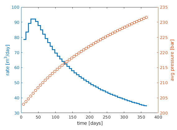
lf
[ha,hr,hp] = ...
   plotyy([sol(2:end).time]/day, [sol(2:end).qS]*day, ...
          [sol(2:end).time]/day, mean([sol(2:end).pressure]/barsa), ...
          'stairs', 'plot');
%set(ha,'FontSize',16);
set(hr,'LineWidth', 2);
set(hp,'LineStyle','none','Marker','o','LineWidth', 1);
xlabel('time [days]');
ylabel(ha(1), 'rate [m^3/day]');
p=get(gca,'Position'); p(1)=p(1)-.01; p(2)=p(2)+.02; set(gca,'Position',p);
ylabel(ha(2), 'avg pressure [bar]');
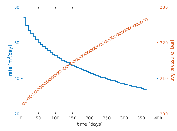
Non-Newtonian fluid
Generated from nonNewtonianFace.m
In this example, we will demonstrate how one can easily extend the compressible single-phase pressure solver to include the effect of non-Newtonian fluids modelled using a simple power law in which the effective viscosity depends on the norm of the velocity
Define geometric quantitites
Grid that represents the reservoir geometry
[nx,ny,nz] = deal( 10,  10, 10);
[Lx,Ly,Lz] = deal(200, 200, 50);
G = cartGrid([nx, ny, nz], [Lx, Ly, Lz]);
G = computeGeometry(G);

% Discrete operators
N  = double(G.faces.neighbors);
intInx = all(N ~= 0, 2);
N  = N(intInx, :);
n = size(N,1);
C = sparse( [(1:n)'; (1:n)'], N, ones(n,1)*[-1 1], n, G.cells.num);
grad = @(x)C*x;
div  = @(x)-C'*x;
avg  = @(x) 0.5 * (x(N(:,1)) + x(N(:,2)));
Rock model and transmissibilities
rock = makeRock(G, 30*milli*darcy, 0.3);

cr   = 1e-6/barsa;
p_r  = 200*barsa;
pv_r = poreVolume(G, rock);
pv   = @(p) pv_r .* exp( cr * (p - p_r) );

hT = computeTrans(G, rock);
cf = G.cells.faces(:,1);
nf = G.faces.num;
T  = 1 ./ accumarray(cf, 1 ./ hT, [nf, 1]);
T  = T(intInx);
fa = G.faces.areas(intInx);
Basic fluid model
c     = 1e-3/barsa;
rho_r = 850*kilogram/meter^3;
rhoS  = 750*kilogram/meter^3;
rho   = @(p) rho_r .* exp( c * (p - p_r) );
if exist('fluidModel', 'var')
   mu0 = fluidModel.mu0;
   nmu = fluidModel.nmu;
   Kc  = fluidModel.Kc;
   Kbc = (Kc/mu0)^(2/(nmu-1))*36*((3*nmu+1)/(4*nmu))^(2*nmu/(nmu-1));
   if nmu==1, Kbc = 0; end
else
   mu0 = 100*centi*poise;
   nmu = 0.25;
   Kc  = .1;
   Kbc = (Kc/mu0)^(2/(nmu-1))*36*((3*nmu+1)/(4*nmu))^(2*nmu/(nmu-1));
end
Initial vertical equilibrium
gravity reset on, g = norm(gravity);
[z_0, z_max] = deal(0, max(G.cells.centroids(:,3)));
equil  = ode23(@(z,p) g .* rho(p), [z_0, z_max], p_r);
p_init = reshape(deval(equil, G.cells.centroids(:,3)), [], 1);  clear equil
Constant for the simulation
numSteps = 52;
totTime  = 365*day;
dt       = totTime / numSteps;
tol      = 1e-5;
maxits   = 100;
Flow equations
phiK   = avg(rock.perm.*rock.poro).*G.faces.areas(intInx).^2;
gradz  = grad(G.cells.centroids(:,3));
v      = @(p, eta)   -(T./(mu0*eta)).*( grad(p) - g*avg(rho(p)).*gradz );
etaEq  = @(p, eta)   eta - (1 + Kbc*v(p,eta).^2./phiK).^((nmu-1)/2);
presEq = @(p, p0, eta, dt)  ...
   (1/dt)*(pv(p).*rho(p) - pv(p0).*rho(p0)) + div(avg(rho(p)).*v(p, eta));
Well model
nperf = 8;
I = repmat(2, [nperf, 1]);
J = (1 : nperf).' + 1;
K = repmat(5, [nperf, 1]);
cellInx = sub2ind(G.cartDims, I, J, K);
W = addWell([ ], G, rock, cellInx, 'Name', 'P1', 'Dir', 'x' );
if exist('wellAvg', 'var') && wellAvg
   wavg = @(eta) 1/6*abs(C(:,W.cells))'*eta;
else
   wavg = @(eta) ones(8,1);
end

% Define well equations
wc = W(1).cells;
WI = W(1).WI;
dz = W(1).dZ;

p_conn = @(bhp) ...
   bhp + g*dz.*rho(bhp);
q_conn = @(p, eta, bhp) ...
   WI .* (rho(p(wc)) ./ (mu0*wavg(eta))) .* (p_conn(bhp) - p(wc));
rateEq = @(p, eta, bhp, qS) ...
   qS - sum(q_conn(p, eta, bhp))/rhoS;
ctrlEq = @(bhp) ...
   bhp - 300*barsa;
Initialize for solution loop
nc = G.cells.num;
nf = numel(T);
[p_ad, eta_ad, bhp_ad, qS_ad] = ...
   initVariablesADI(p_init, ones(nf,1), p_init(wc(1)), 0);
[pIx, etaIx, bhpIx, qSIx] = ...
   deal(1:nc, nc+1:nc+nf, nc+nf+1, nc+nf+2);
sol = repmat(struct('time',[],'pressure',[],'eta',[], ...
                    'bhp',[],'qS',[]), [numSteps+1,1]);
sol(1) = struct('time', 0, 'pressure', value(p_ad), ...
                'eta', value(eta_ad), ...
                'bhp', value(bhp_ad), 'qS', value(qS_ad));
[etamin, etawmin, etamean] = deal(zeros(numSteps,1));
Time loop
t = 0; step = 0;
while t < totTime

   % Increment time
   t = t + dt;
   step = step + 1;
   fprintf('Time step %d: Time %.2f -> %.2f days\n', ...
      step, convertTo(t - dt, day), convertTo(t, day));

   % Main Newton loop
   p0  = value(p_ad); % Previous step pressure
   [resNorm,nit] = deal(1e99, 0);
   while (resNorm > tol) && (nit < maxits)

      % Newton loop for eta (effective viscosity)
      [resNorm2,nit2] = deal(1e99, 0);
      eta_ad2 = initVariablesADI(eta_ad.val);
      while (resNorm2 > tol) && (nit2 <= maxits)
         eeq = etaEq(p_ad.val, eta_ad2);
         res = eeq.val;
         eta_ad2.val = eta_ad2.val - (eeq.jac{1} \ res);

         resNorm2 = norm(res);
         nit2     = nit2+1;
      end
      if nit2 > maxits
         error('Local Newton solves did not converge')
      else
         eta_ad.val = eta_ad2.val;
      end

      % Add source terms to homogeneous pressure equation:
      eq1     = presEq(p_ad, p0, eta_ad, dt);
      eq1(wc) = eq1(wc) - q_conn(p_ad, eta_ad, bhp_ad);

      % Collect all equations
      eqs = {eq1, etaEq(p_ad, eta_ad), ...
         rateEq(p_ad, eta_ad, bhp_ad, qS_ad), ctrlEq(bhp_ad)};

      % Concatenate equations and solve for update:
      eq  = cat(eqs{:});
      J   = eq.jac{1};  % Jacobian
      res = eq.val;     % residual
      upd = -(J \ res); % Newton update
      % Update variables
      p_ad.val   = p_ad.val   + upd(pIx);
      eta_ad.val = eta_ad.val + upd(etaIx);
      bhp_ad.val = bhp_ad.val + upd(bhpIx);
      qS_ad.val  = qS_ad.val  + upd(qSIx);

      resNorm = norm(res);
      nit     = nit + 1;
   end

%   clf,
%   plotFaces(G,intInx, eta_ad.val,'FaceAlpha',.3,'EdgeAlpha', .1);
%   view(3); colorbar; drawnow

   if nit > maxits
      error('Newton solves did not converge')
   else % store solution
      sol(step+1)  = struct('time', t, 'pressure', value(p_ad), ...
         'eta', value(eta_ad), ...
         'bhp', value(bhp_ad), 'qS', value(qS_ad));
   end
   etamin (step) = min(eta_ad.val);
   etawmin(step) = min(wavg(eta_ad.val));
   etamean(step) = mean(eta_ad.val);
end
Time step 1: Time 0.00 -> 7.02 days
Time step 2: Time 7.02 -> 14.04 days
Time step 3: Time 14.04 -> 21.06 days
Time step 4: Time 21.06 -> 28.08 days
Time step 5: Time 28.08 -> 35.10 days
Time step 6: Time 35.10 -> 42.12 days
Time step 7: Time 42.12 -> 49.13 days
Time step 8: Time 49.13 -> 56.15 days
...
lf
[ha,hr,hp] = ...
   plotyy([sol(2:end).time]/day, [sol(2:end).qS]*day, ...
          [sol(2:end).time]/day, mean([sol(2:end).pressure]/barsa), ...
          'stairs', 'plot');
%set(ha,'FontSize',16);
set(hr,'LineWidth', 2);
set(hp,'LineStyle','none','Marker','o','LineWidth', 1);
xlabel('time [days]');
ylabel(ha(1), 'rate [m^3/day]');
p=get(gca,'Position'); p(1)=p(1)-.01; p(2)=p(2)+.02; set(gca,'Position',p);
ylabel(ha(2), 'avg pressure [bar]');
mu0 = 100*centi*poise;
for nsim=1:4
   switch nsim
      case 1
         fluidModel = struct('mu0', mu0, 'nmu',  1, 'Kc', .1);
         nonNewtonianCell;
      case 2
         fluidModel = struct('mu0', mu0, 'nmu', .3, 'Kc', .1);
         nonNewtonianCell;
      case 3
         fluidModel = struct('mu0', mu0, 'nmu', .3, 'Kc', .1);
         wellAvg = true;
         nonNewtonianFace;
      case 4
         fluidModel = struct('mu0', mu0, 'nmu', .3, 'Kc', .1);
         wellAvg = false;
         nonNewtonianFace;
   end
   avgpres(:,nsim) = mean([sol(2:end).pressure]/barsa);        %#ok<SAGROW>
   rate   (:,nsim) = [sol(2:end).qS]*day;                      %#ok<SAGROW>
   time   (:,nsim) = [sol(2:end).time]/day;                    %#ok<SAGROW>
   mineta (:,nsim) = etamin;                                   %#ok<SAGROW>
   minweta(:,nsim) = etawmin;                                  %#ok<SAGROW>
   meaneta(:,nsim) = etamean;                                  %#ok<SAGROW>
end
Time step 1: Time 0.00 -> 7.02 days
Time step 2: Time 7.02 -> 14.04 days
Time step 3: Time 14.04 -> 21.06 days
Time step 4: Time 21.06 -> 28.08 days
Time step 5: Time 28.08 -> 35.10 days
Time step 6: Time 35.10 -> 42.12 days
Time step 7: Time 42.12 -> 49.13 days
Time step 8: Time 49.13 -> 56.15 days
...
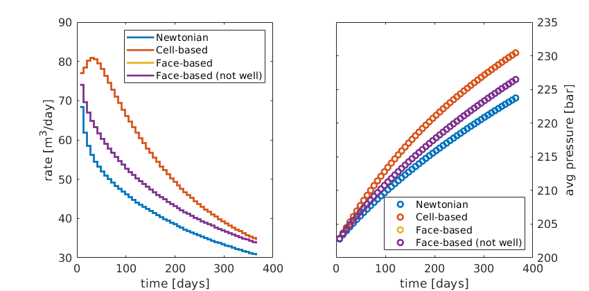
figure('Position', [440 375 840 420]);
subplot(1,2,1);
stairs(time, rate, 'LineWidth', 2);
set(gca,'FontSize',12);
xlabel('time [days]'); ylabel('rate [m^3/day]');
legend('Newtonian', 'Cell-based', 'Face-based', 'Face-based (not well)', ...
       'Location', 'NorthEast');
subplot(1,2,2);
plot(time, avgpres,'o','LineWidth', 2);
set(gca,'FontSize',12,'YAxisLocation','right');
xlabel('time [days]'); ylabel('avg pressure [bar]');
legend('Newtonian', 'Cell-based', 'Face-based', 'Face-based (not well)', ...
       'Location', 'SouthEast');
set(gcf,'PaperPositionMode','auto');
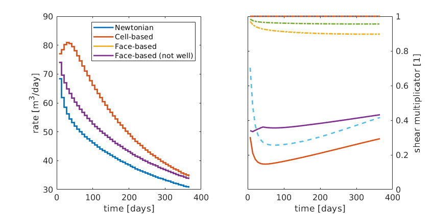
ubplot(1,2,2), cla
plot(time,mineta,'-','LineWidth',2);
hold on
plot(time,minweta,'--','LineWidth',2);
plot(time,meaneta,'-.','LineWidth',2);
hold off
set(gca,'FontSize',12,'YAxisLocation','right');
xlabel('time [days]'); ylabel('shear multiplicator [1]');
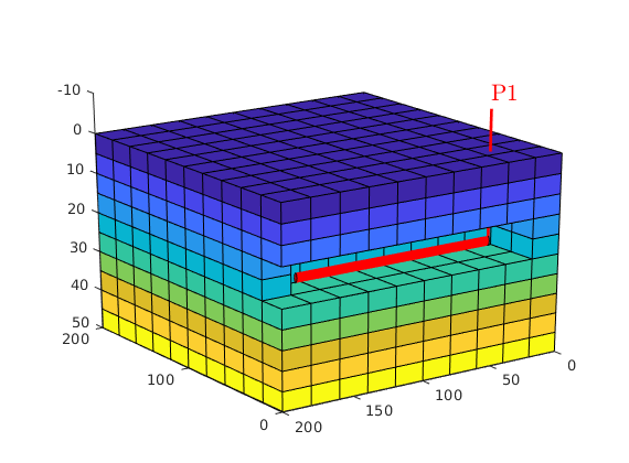
Single-phase compressible AD solver
Generated from singlePhaseAD.m
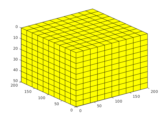
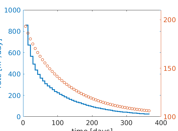
The purpose of the example is to give the first introduction to how one can use the automatic differentiation (AD) class in MRST to write a flow simulator for a compressible single-phase model. For simplicity, the reservoir is assumed to be a rectangular box with homogeneous properties and no-flow boundaries. Starting from a hydrostatic initial state, the reservoir is produced from a horizontal well that will create a zone of pressure draw-down. As more fluids are produced, the average pressure in the reservoir drops, causing a gradual decay in the production rate.
Set up model geometry
[nx,ny,nz] = deal( 10,  10, 10);
[Dx,Dy,Dz] = deal(200, 200, 50);
G = cartGrid([nx, ny, nz], [Dx, Dy, Dz]);
G = computeGeometry(G);

plotGrid(G); view(3); axis tight
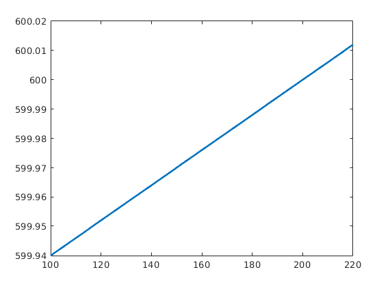
Define rock model
rock = makeRock(G, 30*milli*darcy, 0.3);

cr   = 1e-6/barsa;
p_r  = 200*barsa;
pv_r = poreVolume(G, rock);
pv   = @(p) pv_r .* exp( cr * (p - p_r) );

p = linspace(100*barsa,220*barsa,50);
plot(p/barsa, pv_r(1).*exp(cr*(p-p_r)),'LineWidth',2);
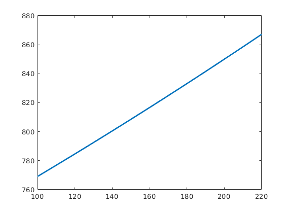
Define model for compressible fluid
mu    = 5*centi*poise;
c     = 1e-3/barsa;
rho_r = 850*kilogram/meter^3;
rhoS  = 750*kilogram/meter^3;
rho   = @(p) rho_r .* exp( c * (p - p_r) );

plot(p/barsa,rho(p),'LineWidth',2);
Assume a single horizontal well
nperf = 8;
I = repmat(2, [nperf, 1]);
J = (1 : nperf).' + 1;
K = repmat(5, [nperf, 1]);
cellInx = sub2ind(G.cartDims, I, J, K);
W = addWell([ ], G, rock, cellInx, 'Name', 'P1', 'Dir', 'y' );
Impose vertical equilibrium
gravity reset on, g = norm(gravity);
[z_0, z_max] = deal(0, max(G.cells.centroids(:,3)));
equil  = ode23(@(z,p) g .* rho(p), [z_0, z_max], p_r);
p_init = reshape(deval(equil, G.cells.centroids(:,3)), [], 1);  clear equil
Plot well and initial pressure
clf
show = true(G.cells.num,1);
cellInx = sub2ind(G.cartDims, ...
   [I-1; I-1; I; I;   I(1:2)-1], ...
   [J  ; J;   J; J;   nperf+[2;2]], ...
   [K-1; K;   K; K-1; K(1:2)-[0; 1]]);
show(cellInx) = false;
plotCellData(G,p_init/barsa, show,'EdgeColor','k');
plotWell(G,W, 'height',10);
view(-125,20), camproj perspective

Compute transmissibilities
N  = double(G.faces.neighbors);
intInx = all(N ~= 0, 2);
N  = N(intInx, :);                          % Interior neighbors
hT = computeTrans(G, rock);                 % Half-transmissibilities
cf = G.cells.faces(:,1);
nf = G.faces.num;
T  = 1 ./ accumarray(cf, 1 ./ hT, [nf, 1]); % Harmonic average
T  = T(intInx);                             % Restricted to interior
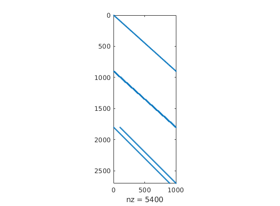
Define discrete operators
n = size(N,1);
C = sparse( [(1:n)'; (1:n)'], N, ones(n,1)*[-1 1], n, G.cells.num);
grad = @(x)C*x;
div  = @(x)-C'*x;
avg  = @(x) 0.5 * (x(N(:,1)) + x(N(:,2)));
spy(C)
Define flow equations
gradz  = grad(G.cells.centroids(:,3));
v      = @(p)  -(T/mu).*( grad(p) - g*avg(rho(p)).*gradz );
presEq = @(p,p0,dt) (1/dt)*(pv(p).*rho(p) - pv(p0).*rho(p0)) ...
                      + div( avg(rho(p)).*v(p) );
Define well equations
wc = W(1).cells; % connection grid cells
WI = W(1).WI;    % well-indices
dz = W(1).dZ;    % connection depth relative to bottom-hole

p_conn  = @(bhp)  bhp + g*dz.*rho(bhp); %connection pressures
q_conn  = @(p,bhp) WI .* (rho(p(wc)) / mu) .* (p_conn(bhp) - p(wc));

rateEq = @(p,bhp,qS)  qS-sum(q_conn(p, bhp))/rhoS;
ctrlEq = @(bhp)       bhp-100*barsa;
Initialize for solution loop
[p_ad, bhp_ad, qS_ad] = initVariablesADI(p_init, p_init(wc(1)), 0);
nc = G.cells.num;
[pIx, bhpIx, qSIx] = deal(1:nc, nc+1, nc+2);

numSteps = 52;                  % number of time-steps
totTime  = 365*day;             % total simulation time
dt       = totTime / numSteps;  % constant time step
tol      = 1e-5;                % Newton tolerance
maxits   = 10;                  % max number of Newton its

sol = repmat(struct('time',[],'pressure',[],'bhp',[],'qS',[]),[numSteps+1,1]);
sol(1)  = struct('time', 0, 'pressure', value(p_ad), ...
   'bhp', value(bhp_ad), 'qS', value(qS_ad));
Main loop
t = 0; step = 0;
hwb = waitbar(t,'Simulation ..');
while t < totTime
   t = t + dt;
   step = step + 1;
   fprintf('\nTime step %d: Time %.2f -> %.2f days\n', ...
      step, convertTo(t - dt, day), convertTo(t, day));
   % Newton loop
   resNorm = 1e99;
   p0  = value(p_ad); % Previous step pressure
   nit = 0;
   while (resNorm > tol) && (nit <= maxits)
      % Add source terms to homogeneous pressure equation:
      eq1     = presEq(p_ad, p0, dt);
      eq1(wc) = eq1(wc) - q_conn(p_ad, bhp_ad);
      % Collect all equations
      eqs = {eq1, rateEq(p_ad, bhp_ad, qS_ad), ctrlEq(bhp_ad)};
      % Concatenate equations and solve for update:
      eq  = cat(eqs{:});
      J   = eq.jac{1};  % Jacobian
      res = eq.val;     % residual
      upd = -(J \ res); % Newton update
      % Update variables
      p_ad.val   = p_ad.val   + upd(pIx);
      bhp_ad.val = bhp_ad.val + upd(bhpIx);
      qS_ad.val  = qS_ad.val  + upd(qSIx);

      resNorm = norm(res);
      nit     = nit + 1;
      fprintf('  Iteration %3d:  Res = %.4e\n', nit, resNorm);
   end

   if nit > maxits
      error('Newton solves did not converge')
   else % store solution
      sol(step+1)  = struct('time', t, 'pressure', value(p_ad), ...
                            'bhp', value(bhp_ad), 'qS', value(qS_ad));
      waitbar(t/totTime,hwb);
   end
end
close(hwb);
Time step 1: Time 0.00 -> 7.02 days
  Iteration   1:  Res = 1.0188e+07
  Iteration   2:  Res = 3.1032e-02
  Iteration   3:  Res = 1.8547e-05
  Iteration   4:  Res = 5.4513e-12

Time step 2: Time 7.02 -> 14.04 days
...
Plot production rate and pressure decay
clf,
[ha,hr,hp] = plotyy(...
   [sol(2:end).time]/day, -[sol(2:end).qS]*day, ...
   [sol(2:end).time]/day, mean([sol(2:end).pressure]/barsa), 'stairs', 'plot');
set(ha,'FontSize',16);
set(hr,'LineWidth', 2);
set(hp,'LineStyle','none','Marker','o','LineWidth', 1);
set(ha(2),'YLim',[100 210],'YTick',100:50:200);
xlabel('time [days]');
ylabel(ha(1), 'rate [m^3/day]');
ylabel(ha(2), 'avg pressure [bar]');
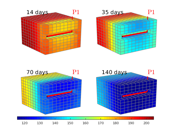
Plot pressure evolution
lf;
steps = [2 5 10 20];
for i=1:4
   subplot(2,2,i);
   set(gca,'Clipping','off');
   plotCellData(G, sol(steps(i)).pressure/barsa, show,'EdgeColor',.5*[1 1 1]);
   plotWell(G,W);
   view(-125,20), camproj perspective
   caxis([115 205]);
   axis tight off; zoom(1.1)
   text(200,170,-8,[num2str(round(steps(i)*dt/day)) ' days'],'FontSize',14);
end
h=colorbar('horiz','Position',[.1 .05 .8 .025]);
colormap(jet(55));
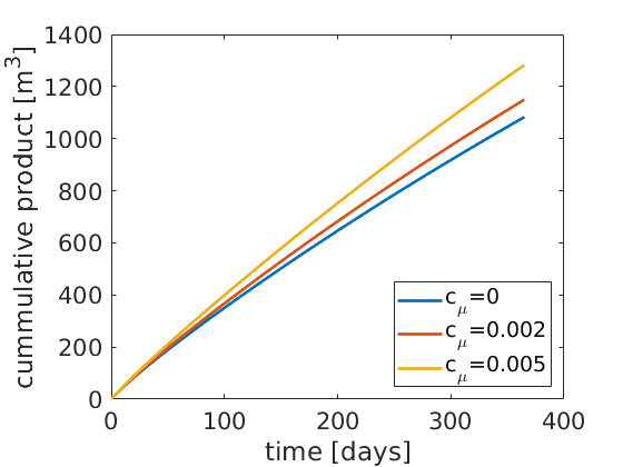
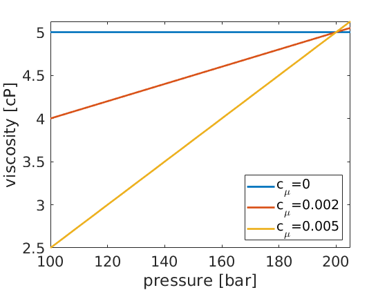
Pressure-dependent viscosity
Generated from singlePhaseMuP.m
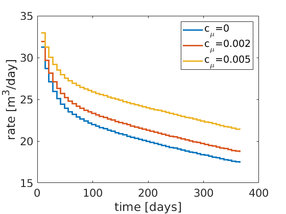
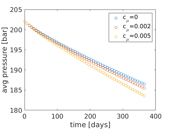
In this example, we will demonstrate how one can easily extend the compressible single-phase pressure solver to include the effect of pressure-dependent viscosity using either arithmetic averaging of the viscosity or harmonic averaging of the fluid mobility.
Define geometric quantitites
Grid that represents the reservoir geometry
[nx,ny,nz] = deal( 10,  10, 10);
[Lx,Ly,Lz] = deal(200, 200, 50);
G = cartGrid([nx, ny, nz], [Lx, Ly, Lz]);
G = computeGeometry(G);

% Discrete operators
N  = double(G.faces.neighbors);
intInx = all(N ~= 0, 2);
N  = N(intInx, :);
n = size(N,1);
C = sparse( [(1:n)'; (1:n)'], N, ones(n,1)*[-1 1], n, G.cells.num);
grad = @(x)C*x;
div  = @(x)-C'*x;
avg  = @(x) 0.5 * (x(N(:,1)) + x(N(:,2)));
Rock model and transmissibilities
rock = makeRock(G, 30*milli*darcy, 0.3);
mrstModule add spe10
rock = getSPE10rock(41:50,101:110,1:10);

cr   = 1e-6/barsa;
p_r  = 200*barsa;
pv_r = poreVolume(G, rock);
pv   = @(p) pv_r .* exp( cr * (p - p_r) );

hT = computeTrans(G, rock);
cf = G.cells.faces(:,1);
nf = G.faces.num;
T  = 1 ./ accumarray(cf, 1 ./ hT, [nf, 1]);
T  = T(intInx);
Fluid model
mu0   = 5*centi*poise;
c     = 1e-3/barsa;
rho_r = 850*kilogram/meter^3;
rhoS  = 750*kilogram/meter^3;
rho   = @(p) rho_r .* exp( c * (p - p_r) );

gravity reset on, g = norm(gravity);
[z_0, z_max] = deal(0, max(G.cells.centroids(:,3)));
equil  = ode23(@(z,p) g .* rho(p), [z_0, z_max], p_r);
p_init = reshape(deval(equil, G.cells.centroids(:,3)), [], 1);  clear equil
Assume a single horizontal well
nperf = 8;
I = repmat(2, [nperf, 1]);
J = (1 : nperf).' + 1;
K = repmat(5, [nperf, 1]);
cellInx = sub2ind(G.cartDims, I, J, K);
W = addWell([ ], G, rock, cellInx, 'Name', 'P1', 'Dir', 'x' );
Main loop
numSteps = 52;
totTime  = 365*day;
dt       = totTime / numSteps;
tol      = 1e-5;
maxits   = 10;
mu_const = [0 2e-3 5e-3]/barsa;
[mypres,myrate] = deal(nan(numSteps+1,2*numel(mu_const)));

n = 1;
for method=1:2

   for i=1:numel(mu_const)

      mu = @(p) mu0*(1+mu_const(i)*(p-p_r));

      gradz = grad(G.cells.centroids(:,3));
      switch method
         case 1
            v  = @(p)  -(T./mu(avg(p))).*( grad(p) - g*avg(rho(p)).*gradz );
         case 2
            hf2cn = getCellNoFaces(G);
            nhf = numel(hf2cn);
            hf2f  = sparse(double(G.cells.faces(:,1)),(1:nhf)',1);
            hf2if = hf2f(intInx,:);
            hlam = @(mu,p) 1./(hf2if*(mu(p(hf2cn))./hT));
            %
            v  = @(p) -hlam(mu,p).*( grad(p) - g*avg(rho(p)).*gradz );
      end

      presEq = @(p, p0, dt) (1/dt)*(pv(p).*rho(p) - pv(p0).*rho(p0)) ...
         + div( avg(rho(p)).*v(p) );

      % Define well equations
      wc = W(1).cells; % connection grid cells
      WI = W(1).WI;    % well-indices
      dz = W(1).dZ;    % connection depth relative to bottom-hole

      p_conn  = @(bhp)  bhp + g*dz.*rho(bhp); %connection pressures
      q_conn  = @(p,bhp) WI .* (rho(p(wc)) ./ mu(p(wc))) .* (p_conn(bhp) - p(wc));

      rateEq = @(p,bhp,qS)  qS-sum(q_conn(p, bhp))/rhoS;
      ctrlEq = @(bhp)       bhp-100*barsa;

      % Initialize for solution loop
      [p_ad, bhp_ad, qS_ad] = initVariablesADI(p_init, p_init(wc(1)), 0);
      nc = G.cells.num;
      [pIx, bhpIx, qSIx] = deal(1:nc, nc+1, nc+2);
      sol = repmat(struct('time',[],'pressure',[],'bhp',[],'qS',[]),[numSteps+1,1]);
      sol(1)  = struct('time', 0, 'pressure', value(p_ad), ...
         'bhp', value(bhp_ad), 'qS', value(qS_ad));

      % Time loop
      t = 0; step = 0;
      hwb = waitbar(0,'Simulation ..');
      while t < totTime
         t = t + dt;
         step = step + 1;
         fprintf('Time step %d: Time %.2f -> %.2f days\n', ...
            step, convertTo(t - dt, day), convertTo(t, day));
         % Newton loop
         resNorm = 1e99;
         p0  = value(p_ad); % Previous step pressure
         nit = 0;
         while (resNorm > tol) && (nit <= maxits)
            % Add source terms to homogeneous pressure equation:
            eq1     = presEq(p_ad, p0, dt);
            eq1(wc) = eq1(wc) - q_conn(p_ad, bhp_ad);
            % Collect all equations
            eqs = {eq1, rateEq(p_ad, bhp_ad, qS_ad), ctrlEq(bhp_ad)};
            % Concatenate equations and solve for update:
            eq  = cat(eqs{:});
            J   = eq.jac{1};  % Jacobian
            res = eq.val;     % residual
            upd = -(J \ res); % Newton update
            % Update variables
            p_ad.val   = p_ad.val   + upd(pIx);
            bhp_ad.val = bhp_ad.val + upd(bhpIx);
            qS_ad.val  = qS_ad.val  + upd(qSIx);

            resNorm = norm(res);
            nit     = nit + 1;
          end

         if nit > maxits
            error('Newton solves did not converge')
         else % store solution
            sol(step+1)  = struct('time', t, 'pressure', value(p_ad), ...
               'bhp', value(bhp_ad), 'qS', value(qS_ad));
           waitbar(t/totTime,hwb)
         end
      end
      close(hwb)
      myrate(2:end,n) = -[sol(2:end).qS]*day;
      mypres(:,n) = mean([sol(:).pressure]/barsa);
      mytime = [sol(1:end).time]/day;
      n = n+1;
   end
end
Time step 1: Time 0.00 -> 7.02 days
Time step 2: Time 7.02 -> 14.04 days
Time step 3: Time 14.04 -> 21.06 days
Time step 4: Time 21.06 -> 28.08 days
Time step 5: Time 28.08 -> 35.10 days
Time step 6: Time 35.10 -> 42.12 days
Time step 7: Time 42.12 -> 49.13 days
Time step 8: Time 49.13 -> 56.15 days
...
igure(1);
myrate(1,:)=NaN;
stairs(mytime, myrate(:,1:3),'LineWidth',2);
set(gca,'FontSize',16);
xlabel('time [days]'); ylabel('rate [m^3/day]');
legend('c_\mu=0', 'c_\mu=0.002', 'c_\mu=0.005');

figure(2);
plot(mytime, mypres(:,1:3),'o');
set(gca,'FontSize',16);
xlabel('time [days]'); ylabel('avg pressure [bar]');
legend('c_\mu=0', 'c_\mu=0.002', 'c_\mu=0.005');

figure(3);
myrate(1,:)=0;
plot(mytime, cumsum(myrate(:,1:3)),'LineWidth',2);
set(gca,'FontSize',16);
xlabel('time [days]'); ylabel('cummulative product [m^3]');
legend('c_\mu=0', 'c_\mu=0.002', 'c_\mu=0.005', 'Location', 'SouthEast');

figure(4);
p = [100*barsa,205*barsa];
mup = zeros(numel(p), numel(mu_const));
for i=1:numel(mu_const)
   mu = @(p) mu0*(1+mu_const(i)*(p-p_r));
   mup(:,i) = mu(p);
end
plot(convertTo(p,barsa),convertTo(mup,centi*poise),'LineWidth',2);
set(gca,'FontSize',16);
xlabel('pressure [bar]'); ylabel('viscosity [cP]');
legend('c_\mu=0', 'c_\mu=0.002', 'c_\mu=0.005', 'Location', 'SouthEast');
axis tight
Single-phase compressible AD solver with thermal effects
Generated from singlePhaseThermal.m
The purpose of the example is to give demonstrate rapid prototying in MRST using the automatic differentiation (AD) class. To this end, we extend the flow simulator for compressible single-phase flow to include temperature effects, which are modeled by incorporating a second conservation equation for energy. Except for this, the computational setup is the same with a single horizontal well draining fluids from a simple box-geometry reservoir.
mrstModule add ad-core
Set up model: grid, perm and poro
[nx,ny,nz] = deal( 10,  10, 10);
[Dx,Dy,Dz] = deal(200, 200, 50);
G = cartGrid([nx, ny, nz], [Dx, Dy, Dz]);
G = computeGeometry(G);
Define rock model
rock = makeRock(G, 30*milli*darcy, 0.3);

cr   = 1e-6/barsa;
p_r  = 200*barsa;
pv_r = poreVolume(G, rock);
pv   = @(p) pv_r .* exp( cr * (p - p_r) );
sv   = @(p) G.cells.volumes - pv(p);
Define model for compressible fluid
mu0   = 5*centi*poise;
cmup  = 2e-3/barsa;
cmut  = 1e-3;
T_r   = 300;
mu    = @(p,T)  mu0*(1+cmup*(p-p_r)).*exp(-cmut*(T-T_r));

beta  = 1e-3/barsa;
alpha = 5e-3;
rho_r = 850*kilogram/meter^3;
rho_S = 750*kilogram/meter^3;
rho   = @(p,T) rho_r .* (1+beta*(p-p_r)).*exp(-alpha*(T-T_r) );
Quantities for energy equation
Cp = 4e3;
Cr = 2*Cp;
Hf = @(p,T) Cp*T+(1-T_r*alpha).*(p-p_r)./rho(p,T);
Ef = @(p,T) Hf(p,T) - p./rho(p,T);
Er = @(T)   Cp*T;
Assume a single horizontal well
nperf = floor(G.cartDims(2)*(ny-2)/ny);
I = repmat(2, [nperf, 1]);
J = (1 : nperf).' + 1;
K = repmat(nz/2, [nperf, 1]);
cellInx = sub2ind(G.cartDims, I, J, K);
W = addWell([ ], G, rock, cellInx, 'Name', 'P1', 'Dir', 'y');
Impose vertical equilibrium
gravity reset on; g = norm(gravity);
[z_0, z_max] = deal(0, max(G.cells.centroids(:,3)));
equil  = ode23(@(z,p) g.* rho(p,T_r), [z_0, z_max], p_r);
p_init = reshape(deval(equil, G.cells.centroids(:,3)), [], 1);  clear equil
T_init = ones(G.cells.num,1)*T_r;
Plot well and initial pressure
figure
show = true(G.cells.num,1);
cellInx = sub2ind(G.cartDims, ...
   [I-1; I-1; I; I;   I(1:2)-1], ...
   [J  ; J;   J; J;   nperf+[2;2]], ...
   [K-1; K;   K; K-1; K(1:2)-[0; 1]]);
show(cellInx) = false;
plotCellData(G,p_init/barsa, show,'EdgeColor','k');
plotWell(G,W, 'height',10);
view(-125,20), camproj perspective
Compute transmissibilities
N   = double(G.faces.neighbors);
intInx = all(N ~= 0, 2);
cf  = G.cells.faces(:,1);
nf  = G.faces.num;
N   = N(intInx, :);                           % Interior neighbors

hT  = computeTrans(G, rock);                  % Half-transmissibilities
Tp  = 1 ./ accumarray(cf, 1 ./ hT, [nf, 1]);  % Harmonic average
Tp  = Tp(intInx);                             % Restricted to interior

kap = 4;                                      % Heat conduction of granite
tmp = struct('perm',kap*ones(G.cells.num,1)); % Temporary rock object
hT  = computeTrans(G, tmp);                   % Half-transmissibilities
Th  = 1 ./ accumarray(cf, 1 ./ hT, [nf, 1]);  % Harmonic average
Th  = Th(intInx);                             % Restricted to interior
Define discrete operators
n    = size(N,1);
C    = sparse( [(1:n)'; (1:n)'], N, ones(n,1)*[-1 1], n, G.cells.num);
grad = @(x) C*x;
div  = @(x) -C'*x;
avg  = @(x) 0.5 * (x(N(:,1)) + x(N(:,2)));
upw  = @(x,flag) x(N(:,1)).*double(flag)+x(N(:,2)).*double(~flag);
Define flow equations
Writing in functional form means that v(p,T) is evaluated two times more than strictly needed if the whole definition of discrete equations written as a single function
gdz = grad(G.cells.centroids)*gravity()';
v   = @(p,T)  -(Tp./mu(avg(p),avg(T))).*(grad(p) - avg(rho(p,T)).*gdz);
pEq = @(p,T, p0,T0, dt) ...
     (1/dt)*(pv(p).*rho(p,T) - pv(p0).*rho(p0,T0)) ...
      + div( avg(rho(p,T)).*v(p,T) );
hEq = @(p, T, p0, T0, dt) ...
     (1/dt)*(pv(p ).*rho(p, T ).*Ef(p ,T ) + sv(p ).*Er(T ) ...
           - pv(p0).*rho(p0,T0).*Ef(p0,T0) - sv(p0).*Er(T0)) ...
     + div( upw(Hf(p,T),v(p,T)>0).*avg(rho(p,T)).*v(p,T) ) ...
     + div( -Th.*grad(T));
Define well equations.
wc = W(1).cells; % connection grid cells
assert(numel(wc)==numel(unique(wc))); % each cell should only appear once
WI  = W(1).WI;    % well-indices
dz  = W(1).dZ;    % connection depth relative to bottom-hole
bhT = ones(size(wc))*200; % temperature of wells not used if production

p_conn  = @(bhp,bhT) bhp + g*dz.*rho(bhp,bhT); %connection pressures
q_conn  = @(p,T, bhp) ...
    WI .* (rho(p(wc),T(wc))./mu(p(wc),T(wc))) .* (p_conn(bhp,bhT)-p(wc));

rateEq = @(p,T, bhp, qS)  qS-sum(q_conn(p, T, bhp))/rho_S;
ctrlEq = @(bhp)           bhp-100*barsa;
Initialize for solution loop
[p_ad, T_ad, bhp_ad, qS_ad] = ...
    initVariablesADI(p_init,T_init, p_init(wc(1)), 0);
nc = G.cells.num;
[pIx, TIx, bhpIx, qSIx] = deal(1:nc, nc+1:2*nc, 2*nc+1, 2*nc+2);

numSteps = 78;                  % number of time-steps
totTime  = 365*day*1.5;         % total simulation time
dt       = totTime / numSteps;  % constant time step
tol      = 1e-5;                % Newton tolerance
maxits   = 10;                  % max number of Newton its

sol = repmat(struct('time',[], 'pressure',[], 'bhp',[], 'qS',[], ...
    'T',[], 'qH',[]),[numSteps+1,1]);
sol(1)  = struct('time', 0, 'pressure', value(p_ad), ...
    'bhp', value(bhp_ad), 'qS', value(qS_ad), 'T', value(T_ad),'qH', 0);
Main loop
t = 0; step = 0;
hwb = waitbar(0,'Simulation..');
while t < totTime
   t = t + dt;
   step = step + 1;
   fprintf('\nTime step %d: Time %.2f -> %.2f days\n', ...
      step, convertTo(t - dt, day), convertTo(t, day));

   % Newton loop
   resNorm = 1e99;
   p0  = value(p_ad); % Previous step pressure
   T0  = value(T_ad);
   nit = 0;
   while (resNorm > tol) && (nit < maxits)

      % Add source terms to homogeneous pressure equation:
      eq1      = pEq(p_ad,T_ad, p0, T0,dt);
      qw       = q_conn(p_ad,T_ad, bhp_ad);
      eq1(wc)  = eq1(wc) - qw;
      hq       = Hf(bhp_ad,bhT).*qw;    %inflow not in this example
      Hcells   = Hf(p_ad,T_ad);
      hq(qw<0) = Hcells(wc(qw<0)).*qw(qw<0);
      eq2      = hEq(p_ad,T_ad, p0, T0,dt);
      eq2(wc)  = eq2(wc) - hq;

      % Collect all equations. Scale residual of energy equation
      eqs = {eq1, eq2/Cp, rateEq(p_ad,T_ad, bhp_ad, qS_ad), ctrlEq(bhp_ad)};

      % Concatenate equations and solve for update:
      eq  = cat(eqs{:});
      J   = eq.jac{1};  % Jacobian
      res = eq.val;     % residual
      upd = -(J \ res); % Newton update

      % Update variables
      p_ad.val   = p_ad.val   + upd(pIx);
      T_ad.val   = T_ad.val   + upd(TIx);
      bhp_ad.val = bhp_ad.val + upd(bhpIx);
      qS_ad.val  = qS_ad.val  + upd(qSIx);

      resNorm = norm(res);
      nit     = nit + 1;
      fprintf('  Iteration %3d:  Res = %.4e\n', nit, resNorm);
   end

   if nit > maxits
      error('Newton solves did not converge')
   else % store solution
      sol(step+1)  = struct('time', t, 'pressure', value(p_ad), ...
                            'bhp', value(bhp_ad), 'qS', value(qS_ad), ...
                          'T', value(T_ad), 'qH', sum(value(hq)));
      waitbar(t/totTime,hwb);
   end
end
close(hwb)
Time step 1: Time 0.00 -> 7.02 days
  Iteration   1:  Res = 1.0188e+07
  Iteration   2:  Res = 2.9454e+02
  Iteration   3:  Res = 3.9794e+02
  Iteration   4:  Res = 5.8886e+01
  Iteration   5:  Res = 1.3027e+00
  Iteration   6:  Res = 5.9547e-04
...
Plot production rate
clf, set(gca,'FontSize',20);
stairs([sol(2:end).time]/day,-[sol(2:end).qS]*day,'LineWidth',2);
xlabel('days');ylabel('m^3/day')
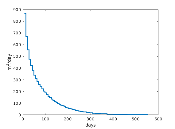
Plot pressure evolution
figure; clf;
steps = [2 5 10 25];
%steps = floor(1:(numel(sol)/6-eps):numel(sol));
p = vertcat(sol(:).pressure);
cax=[min(p) max(p)]./barsa;
for i=1:4
   subplot(2,2,i);
   set(gca,'Clipping','off');
   plotCellData(G, sol(steps(i)).pressure/barsa, show, 'EdgeColor',.5*[1 1 1]);
   plotWell(G, W, 'FontSize',12);
   view(-125,20), camproj perspective
   caxis(cax);
   axis tight off; zoom(1.1)
   text(200,170,-8,[num2str(round(steps(i)*dt/day)) ' days'],'FontSize',12);
end
colorbar('horiz','Position',[.1 .05 .8 .025]);
colormap(jet(55));
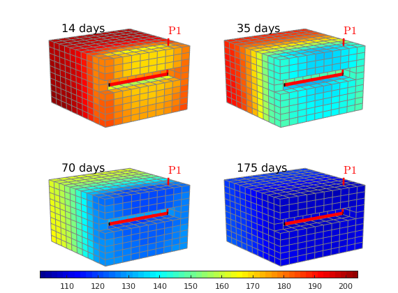
figure(),clf;
steps = [2 5 10 numel(sol)];
T = vertcat(sol(:).T); %-T_r;
cax=[min(T) max(T)];
for i=1:numel(steps)
   subplot(2,2,i);
   set(gca,'Clipping','off');
   plotCellData(G, sol(steps(i)).T, show, 'EdgeColor',.5*[1 1 1]);
   plotWell(G, W, 'FontSize',12);
   view(-125,20), camproj perspective
   caxis(cax);
   axis tight off; zoom(1.1)
   text(200,170,-8,[num2str(round(steps(i)*dt/day)) ' days'],'FontSize',12);
end
h=colorbar('horiz','Position',[.1 .05 .8 .025]);
colormap(jet(55));
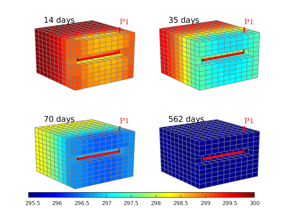
ns = numel(sol);
Tw = nan(ns,numel(wc));
Pw = nan(ns,numel(wc));
[t,Pm,PM,Pa,Tm,TM,Ta] = deal(nan(ns,1));
for i=1:numel(sol)
   t(i) = sol(i).time/day;
   Tw(i,:)=sol(i).T(wc);
   Tm(i) = min(sol(i).T);
   TM(i) = max(sol(i).T);
   Ta(i) = mean(sol(i).T);
   Pw(i,:)=sol(i).pressure(wc)./barsa;
   Pm(i) = min(sol(i).pressure./barsa);
   PM(i) = max(sol(i).pressure./barsa);
   Pa(i) = mean(sol(i).pressure./barsa);
end
figure; plot(t,Pm,t,Pa,t,PM,t,Pw,'.k','LineWidth',2);
legend('min(p)', 'avg(p)', 'max(p)', 'wells');
figure; plot(t,Tm,t,Ta,t,TM,t,Tw,'.k','LineWidth',2);
legend('min(T)', 'avg(T)', 'max(T)', 'wells');
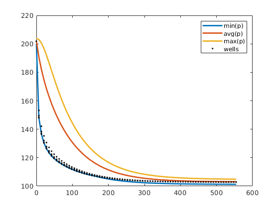
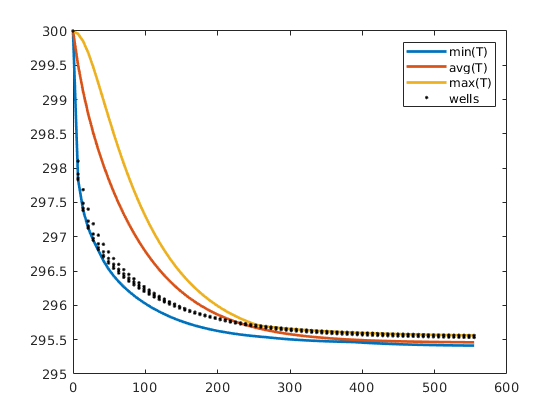
Compute the three different expansion temperatures
[p,T] = initVariablesADI(p_r,T_r);
dp   = Pm(end)*barsa-p_r;

% Joule-Thomson
hf   = Hf(p,T);
dHdp = hf.jac{1};
dHdT = hf.jac{2};
Tjt  = T_r - dHdp*dp/dHdT;
hold on, plot(t([1 end]), [Tjt Tjt],'--k'); hold off
text(t(5), Tjt+.25, 'Joule-Tompson');

% linearized adiabatic temperature
hf   = Ef(p,T) + value(p)./rho(p,T);
dHdp = hf.jac{1};
dHdT = hf.jac{2};
Tab  = T_r - dHdp*dp/dHdT;
hold on, plot(t([1 end]), [Tab Tab],'--k'); hold off
text(t(2), Tab-.35, 'Adiabatic expansion');

% free expansion
hf = Ef(p,T);
dHdp = hf.jac{1};
dHdT = hf.jac{2};
Tfr  = T_r - dHdp*dp/dHdT;
hold on, plot(t([1 end]), [Tfr Tfr],'--k'); hold off
text(t(end/2), Tfr+.25, 'Free expansion');
set(gca,'XLim',t([1 end]));
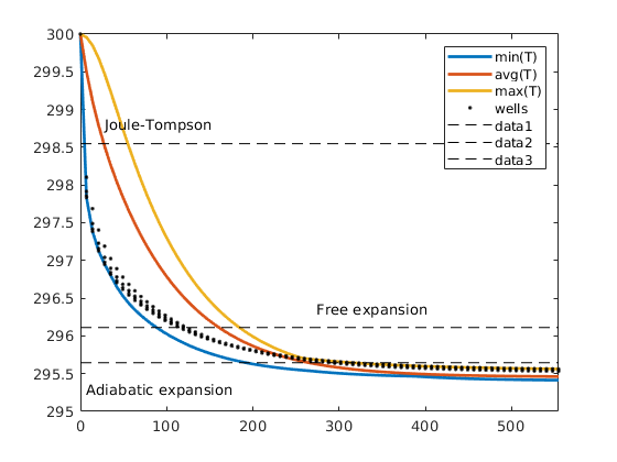
%{
Lorenz coefficient for layers of SPE 10, Model 2
Generated from computeLorenzSPE10.m
In this example, we first compute the Lorenz coefficient for all layers of the SPE10 model subject to a five-spot well pattern. We then pick one of the layers and show how we can balance the well allocation and improve the Lorenz coefficient and the areal sweep by moving some of the wells to regions with better sand quality.
mrstModule add diagnostics spe10 incomp
Base model
We set up a grid. Later, we will assign petrophysical properties from one single layer at the time to compute Lorenz coefficients inside the main loop
cartDims = [  60,  220,  1];
physDims = [1200, 2200, 2*cartDims(end)] .* ft();
G  = cartGrid(cartDims, physDims);
G  = computeGeometry(G);

% Set parameters describing the
wtype    = {'bhp', 'bhp', 'bhp', 'bhp', 'bhp'};
wtarget  = [200,   200,   200,   200,   500] .* barsa();
wrad     = [0.125, 0.125, 0.125, 0.125, 0.125] .* meter;
wloc     = [  1,   60,     1,   60,  30;
              1,    1,   220,  220, 111];
wname    = {'P1', 'P2', 'P3', 'P4', 'I'};

% Set fluid model: Here, we use a simple fluid model with properties that
% are typical for water. Replace this by a multiphase fluid object if you
% also want to include fluid effects in the calculation
fluid = initSingleFluid('mu', 1*centi*poise, ...
                        'rho', 1014*kilogram/meter^3);
Compute Lorenz coefficient for each layer
Lc = zeros(85,1);
h = waitbar(0,'Computing Lorenz coefficients ...');
for n=1:85

    % --- Set petrophysical data for this particular layer
    % To avoid problems with very small porosity values, we explicitly
    % impose a lower threshold of 1e-4
    rock = getSPE10rock(1:cartDims(1),1:cartDims(2),n);
    rock.poro = max(rock.poro, 1e-4);

    % --- Set up well model
    % To ensure that we get the correct well index when updating the
    % petrophysical data, we simply regenerate the well objects.
    W = [];
    for w = 1 : numel(wtype)
        W = verticalWell(W, G, rock, wloc(1,w), wloc(2,w), 1, ...
            'Type', wtype{w}, 'Val', wtarget(w), ...
            'Radius', wrad(w), 'Name', wname{w}, ...
            'InnerProduct', 'ip_tpf', 'Comp_i', 1);
    end

    % --- Initiate and solve flow problem
    rS = initState(G, W, 0, 0.0);
    T  = computeTrans(G, rock);
    rS = incompTPFA(rS, G, T, fluid, 'wells', W);

    % --- Compute flow diagnostics
    D       = computeTOFandTracer(rS, G, rock, 'wells', W, 'maxTOF', inf);
    [F,Phi] = computeFandPhi(poreVolume(G,rock), D.tof);
    Lc(n)   = computeLorenz(F,Phi);
    waitbar(n/85);
end
close(h);
clf; set(gcf,'Position',[470 420 900 250]);
h=bar(Lc,'hist');
axis tight; set(h,'FaceColor',[.95 .95 1],'EdgeColor',[0 0 .7]);
hold on, h=plot([35.5 35.5],[0 .75],'--k','LineWidth',2); hold off;
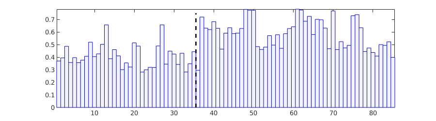
Improve Lorenz/sweep by moving wells
Here, we have first computed Lorenz coefficient, sweep and well-pair connections for the layer with lowest/highest Lorenz coefficient and then tried to move the wells having small allocation factors to the nearest high-poro region that seems reasonably well connected with the injector.
minCase = false;  %#ok<*UNRCH>
if minCase
    [~,n]=min(Lc);
else
    [~,n]=max(Lc);
end
rock = getSPE10rock(1:cartDims(1),1:cartDims(2),n);
rock.poro = max(rock.poro, 1e-4);
pv = poreVolume(G, rock);

nwloc = wloc;
fig1=figure('Position',[250 490 750 300]); col = {'b','g'};
for nstep=1:2
    % Set well conditions
    W = [];
    for w = 1 : numel(wtype)
        W = verticalWell(W, G, rock, nwloc(1,w), nwloc(2,w), 1, ...
            'Type', wtype{w}, 'Val', wtarget(w), ...
            'Radius', wrad(w), 'Name', wname{w}, ...
            'InnerProduct', 'ip_tpf');
    end

    % Compute flow field and diagnostics
    rS = initState(G, W, 0);
    T  = computeTrans(G, rock);
    rS = incompTPFA(rS, G, T, fluid, 'wells', W);
    D  = computeTOFandTracer(rS, G, rock, 'wells', W, 'maxTOF', inf);
    WP = computeWellPairs(rS, G, rock, W, D);
    [F,Phi] = computeFandPhi(pv, D.tof);
    computeLorenz(F,Phi)
    [Ev,tD] = computeSweep(F, Phi);

    % Plot F-Phi and sweep diagram
    % To reduce the number of points, we resample the data
    figure(fig1);
    subplot(1,2,1); hold on;
    xq = linspace(0,1,100);
    vq = interp1(Phi,F,xq);
    plot(xq,vq,['-',col{nstep}],'LineWidth',2); hold off;

    subplot(1,2,2); hold on;
    [T,ia] = unique(tD);
    E = Ev(ia);
    xq = linspace(0,5+(1-minCase)*20,100);
    vq = interp1(T,E,xq);
    plot(xq,vq,['-',col{nstep}],'LineWidth',2); hold off;

    % Plot porosity map and well-pair connections
    figure('Position',[710   420   720   400]);
    plotCellData(G,rock.poro,'EdgeColor','none');
    plotWell(G,W,'height',10,'LineWidth',4);
    plotWellPairConnections(G,WP,D,W,pv,1e-4);
    cmap=jet(128); colormap(.4*cmap + .6*ones(size(cmap))); clear cmap;
    view(0,70); set(gca,'DataAspectRatio',[1 1 .5]); axis off
    cax = caxis;

    % Plot zoom around each producer in separate axes
    pos = [.05 .05 .25 .35;  .725 .05 .25 .35; ...
        .05 .6 .25 .35; .725 .6 .25 .35];
    for i=1:4
        axes('position', pos(i,:));
        if nstep==1
            rad(:,i) = sum(bsxfun(@minus,G.cells.centroids,....
                G.cells.centroids(W(i).cells,:)).^2,2); %#ok<SAGROW>
        end
        plotCellData(G,rock.poro,rad(:,i)<3500,'EdgeColor','k','EdgeAlpha',.1);
        plotWell(G,W(i),'height',10,'LineWidth',10);
        caxis(cax);
        view(0,70); set(gca,'DataAspectRatio',[1 1 .5]); axis off tight;
    end

    % Impose manually improved well positions for next pass
    if minCase
        nwloc     = [  1,   53,     1,   59,  30;
                       1,    2,   218,  220, 111];
    else
        nwloc     = [  1,   60,     7,   60,  30;
                       6,   11,   220,  219, 111];
    end
    vertcat(rS.wellSol.flux)
end
figure(fig1);
subplot(1,2,1); hold on; plot([0 1],[0 1],'k'); hold off; title('Lorenz');
subplot(1,2,2); set(gca,'XLim',[0 5+(1-minCase)*20]); title('Sweep');
Warning: Inconsistent Number of Phases.  Using 1 Phase (=min([3, 1, 1])).

ans =

    0.7820


ans =
...
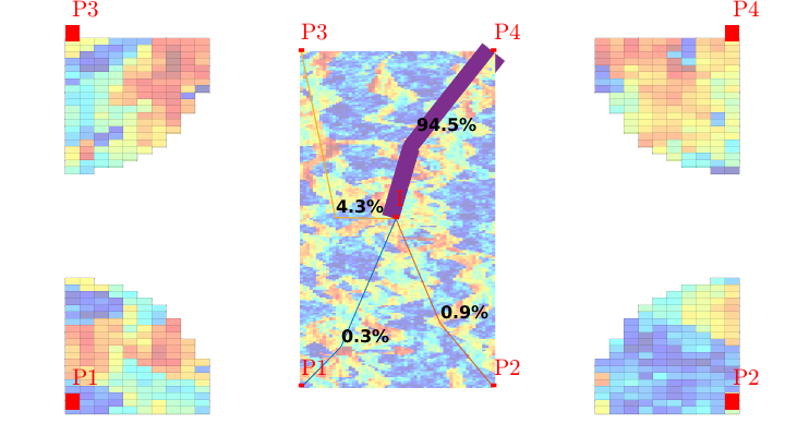
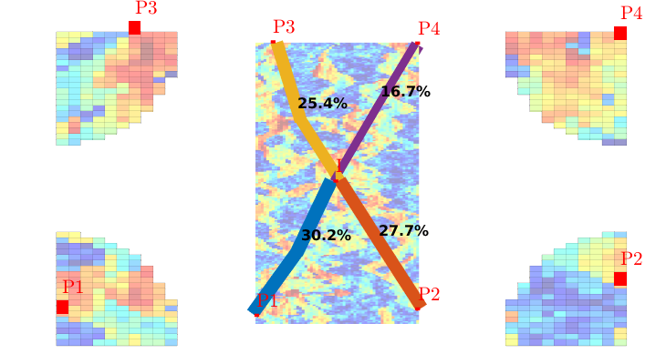
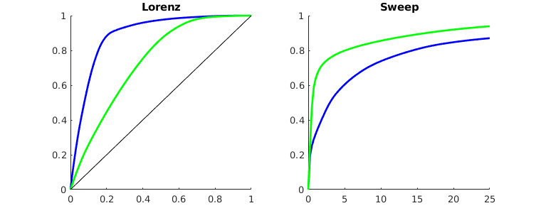
Example: Interactive Diagnostics Tool for the SAIGUP Model
Generated from interactiveSAIGUP.m
In this example, we will use the SAIGUP model as set up in the ‘saigupWithWells’ example to show how to launch an interactive session for doing flow diagnostics.
mrstModule add book diagnostics;
Set up model
We start by re-running this case study to set up the simulation model and compute a flow field. Henceforth, we only need the geological model, the description of the wells, and the reservoir state. Hence, we clear all other variables and close all plots produced by the script.
saigupWithWells;
close all;
clearvars -except G rock W state

% Get rid of LaTeX notation in well names
% In the original example, we used LaTeX syntax to specify well names of
% the form $I_1$, $P_1$, etc. Unfortunately, this does not play very well
% along with MATLAB's tools for  graphical interfaces, and we therefore
% post-process the well names to be on the form I1, P1, etc.
for i=1:numel(W)
    W(i).name = W(i).name([1 5]);
end
Launch flow diagnostics
interactiveDiagnostics(G, rock, W, 'state', state, 'computeFlux', false);
set(gcf,'position',[440 317 866 480]); axis normal
view(-85,73)
New state encountered, computing diagnostics...
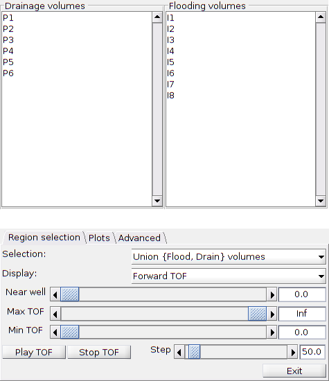
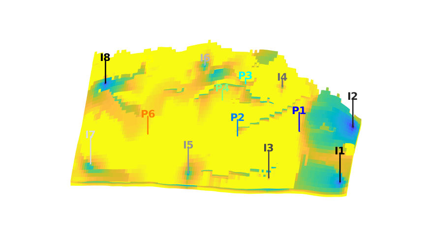
Flux allocation plots
To produce the flux and well allocation figure in the book: - in the ‘region selection’ tab: set maxTOF to zero to remove plotting of volumetric quantities - in the ‘advanced’ tab: select ‘show grid’, ‘well pairs’, and ‘plot all wells’. This will produce the overview of the reservoir - use your pointer (mouse) to click on any of the wells to bring up the allocation plots
Snapshots of swept regions
In the ‘advanced’ tab, deselect ‘show grid’, ‘well pairs’, and ‘plot all wells’. Then, in the ‘region selection’ tab: - set ‘selection’ to ‘intersection’ - set ‘display’ to ‘tracer selected injector’ - select wells (mark I6 and P2 to P6, or I4 and P1 to P4) - type ‘shading faceted’ on the command line - rotation, zoom, and translate the plot to get an acceptable view
Simple 2D reservoir with two injectors and three producers
Generated from interactiveSimple.m
This is an examples discussed in the MRST book, which is a continuation of the ‘showDiagnostBasics’ example, in which we have added two low-porosity regions as a simple representation of two sealing faults, moved the two injectors slightly, and switched all wells from rate to bottom-hole pressure control. In the following, we give instructions for how you can use the diagnostic tool to manipulate the well controls to improve the overall sweep of the reservoir.
Set up the geomodel and specify wells
[nx,ny] = deal(64);
G = cartGrid([nx,ny,1],[5000,2500,10]);
G = computeGeometry(G);
p = gaussianField(G.cartDims(1:2), [0.2 0.4], [11 3], 2.5);
p(round(2*end/3):end,round(end/3)) = 1e-3;
p(1:round(end/3),round(2*end/3)) = 1e-3;
K = p.^3.*(1.5e-5)^2./(0.81*72*(1-p).^2);
rock = makeRock(G, K(:), p(:));
Set up and solve flow problem, compute diagnostics
n = 12;
W = addWell([],  G, rock, nx*(n-6)+n/2+1, ...
    'Type', 'bhp', 'Comp_i', 1, 'name', 'I1', 'Val', 200*barsa);
W = addWell(W, G, rock, nx*(n-6)+n/2+1+nx-n, ...
    'Type','bhp',  'Comp_i', 1, 'name', 'I2', 'Val', 200*barsa);
W = addWell(W, G, rock, round(G.cells.num-(n/2-.5)*nx-.3*nx), ...
    'Type','bhp',  'Comp_i', 0, 'name', 'P1', 'Val', 100*barsa);
W = addWell(W, G, rock, G.cells.num-(n-.5)*nx, ...
    'Type','bhp',  'Comp_i', 0, 'name', 'P2', 'Val', 100*barsa);
W = addWell(W, G, rock, round(G.cells.num-(n/2-.5)*nx+.3*nx), ...
    'Type','bhp',  'Comp_i', 0, 'name', 'P3', 'Val', 100*barsa);
close all;
mrstModule add diagnostics
interactiveDiagnostics(G, rock, W, 'showGrid', true);
axis normal tight; view(0,90);
New state encountered, computing diagnostics...
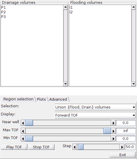
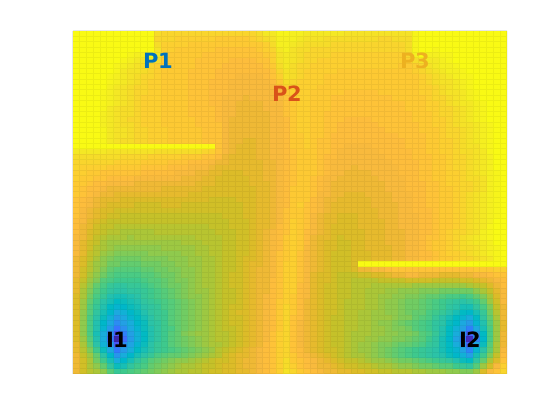
Plot of reservoir model:
Plot of time evolution
- Set display to be ‘forward TOF’, and selection to be ‘Flood volumes’ - set ‘Max TOF’ to be 25, 75, 125, and 175 - or use the ‘Play TOF’ button to play the evolution of neutral displacement fronts
Manual optimization of flow pattern
First, change the colormap to
colormap(gray.^10);
% and then switch the displayed property to be 'sum of tofs'

% From the 'plots' tab, you can first plot the F-Phi diagram, and then say
figure(3); hold on
% to ensure that if you push this button subsequently, the new F-Phi
% diagram will be added on top of the preexisting one(s) rather than
% replacing it. (Depending upon what you have done before you come to this
% point, the number of the figure may be different. Check the window header
% to get the right number.)

% Case 1:
% Use the 'edit wells' button from the 'plots' tab to edit the various
% wells. We can start by increasing the pressure of 'P2' from 100 bar to
% 130 bar to decrease the flow rate in the I1-P2 region. Once you have
% entered the new value (13000000), you push 'apply' and a new flow field
% with flow diagnostics will be computed. You can now change the displayed
% property to be 'sum of TOFs', and use the 'F/Phi diagram' button from the
% 'plots' tab to plot the F-Phi diagram and compute the Lorenz coefficient
% of the new well setup. (To distinguish the curves, you may want to
% manually change the color of the new graph using the 'Edit plot' tool
% from the plotting window.)

% Case 2:
% To increase the flow in the I2-P3 region, we can repeat the exercise and
% set P3 to operate at 80 bar.

% Case 3:
% To also sweep the large unswept region east of P3, we can introduce a new
% well in the south-east of this region, just north of the sealing fault.
% To do this, we use the 'add' button from the 'edit wells' workflow. This
% will bring up a new window in which you can click the cell where you want
% to place the well. When you click a cell, a new window will pop up; this
% can be ignored. Once you are happy with the placement, you close the
% editing window, and then you can sett the correct value in the new well.
% In the book, we propose to set the new well to operate at 140 bar, and
% similarly increase the pressure of I2 to 220 bar. Then you push 'apply',
% go back to view the 'sum of TOFs' and produce a new F-Phi diagram
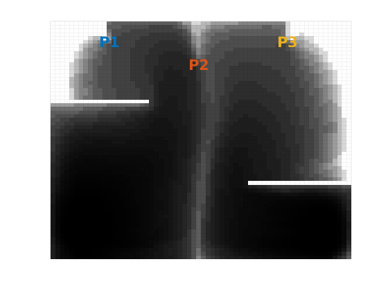

Plot of time evolution
- Set display to be ‘forward TOF’, and selection to be ‘Flood volumes’ - set ‘Max TOF’ to be 25, 75, 125, and 175 - or use the ‘Play TOF’ button to play the evolution of neutral displacement fronts
Exercise:
Can you make any suggestions for further improvements?
Simple Model of an Anticline
Generated from makeAnticlineModel.m
mrstModule add spe10 coarsegrid
Cartesian grid and rock parameters
[nx,ny,nz] = deal(30,30,15);
G = cartGrid([nx ny nz], [nx ny nz].*[20 10 2]*ft);

rock = getSPE10rock(1:nx,1:ny,nz:-1:1);
rock.poro(rock.poro==0) = 1e-5;
%rock.perm = 10*milli*darcy*ones(G.cells.num,1);
%rock.poro = 0.2*ones(G.cells.num,1);
Make anticline structure
x = G.nodes.coords(:,1);
y = G.nodes.coords(:,2);

normalize = @(x) (x-min(x))/(max(x)-min(x));
x = 2*normalize(x)-1;
y = 2*normalize(y)-1;
r = min(sqrt(x.^2 + y.^2),1);
dz = r.^2 ./ (r.^2 + (1-r).^4);

G.nodes.coords(:,3) = G.nodes.coords(:,3) + dz*(nz+1)*2*ft;
G = computeGeometry(G);
Set initial saturation
s = zeros(G.nodes.num,1);
s(G.nodes.coords(:,3)>=nz*2*ft) = 1;
[nodes,pos] = gridCellNodes(G, (1:G.cells.num).');
c = rldecode(1:G.cells.num, diff(pos), 2).';
A = sparse(c,nodes,1)*[s, ones([G.nodes.num,1])];
s = bsxfun(@rdivide, A(:,1:(end-1)), A(:,end));
Set wells
producers
args = {'Type', 'bhp', 'Val', 100*barsa, 'Comp_i', [0 1]};
W = verticalWell([], G, rock, 14, 15, [], args{:}, 'name', 'P1');
W = verticalWell(W,  G, rock, 17, 16, [], args{:}, 'name', 'P2');

% injectors
args = {'Type', 'bhp', 'Val', 150*barsa, 'Comp_i', [1 0]};
W = verticalWell(W,  G, rock,  9,  9, [], args{:}, 'name', 'I1');
W = verticalWell(W,  G, rock,  9, 22, [], args{:}, 'name', 'I2');
W = verticalWell(W,  G, rock, 22,  9, [], args{:}, 'name', 'I3');
W = verticalWell(W,  G, rock, 22, 22, [], args{:}, 'name', 'I4');
mrstModule add diagnostics incomp streamlines;
Set up and solve flow problem
Generated from showDiagnostBasics.m
[nx,ny] = deal(64);
G = cartGrid([nx,ny,1],[500,250,10]);
G = computeGeometry(G);
p = gaussianField(G.cartDims(1:2), [0.2 0.4], [11 3], 2.5);
K = p.^3.*(1.5e-5)^2./(0.81*72*(1-p).^2);
rock = makeRock(G, K(:), p(:));
hT = computeTrans(G, rock);
Set up and solve flow problem, compute diagnostics
gravity reset off
fluid = initSingleFluid('mu', 1*centi*poise, 'rho', 1014*kilogram/meter^3);
pv  = sum(poreVolume(G,rock));

n = 12;
W = addWell([],  G, rock, nx*n+n+1, ...
    'Type', 'rate', 'Comp_i', 1, 'name', 'I1', 'Val', pv/2);
W = addWell(W, G, rock, nx*n+n+1+nx-2*n, ...
    'Type','rate',  'Comp_i', 1, 'name', 'I2', 'Val', pv/2);
W = addWell(W, G, rock, round(G.cells.num-(n/2-.5)*nx-.3*nx), ...
    'Type','rate',  'Comp_i', 0, 'name', 'P1', 'Val', -pv/4);
W = addWell(W, G, rock, G.cells.num-(n-.5)*nx, ...
    'Type','rate',  'Comp_i', 0, 'name', 'P2', 'Val', -pv/2);
W = addWell(W, G, rock, round(G.cells.num-(n/2-.5)*nx+.3*nx), ...
    'Type','rate',  'Comp_i', 0, 'name', 'P3', 'Val', -pv/4);
state = initState(G, W, 0.0, 1.0);
state = incompTPFA(state, G, hT, fluid, 'wells', W);
D = computeTOFandTracer(state, G, rock, 'wells', W);
Warning: Well rates and flux bc must sum up to 0
when there are no bhp constrained wells or pressure bc.Results may not be
reliable.
Trace streamlines
seed = (nx*ny/2 + (1:nx)).';
Sf = pollock(G, state, seed, 'substeps', 1);
Sb = pollock(G, state, seed, 'substeps', 1, 'reverse', true);
Forward time-of-flight
clf
hf=streamline(Sf);
hb=streamline(Sb);
plotGrid(G,vertcat(W.cells),'FaceColor','none','EdgeColor','r','LineWidth',1.5);
plotWell(G,W,'FontSize',20);
set([hf; hb],'Color','w','LineWidth',1.5);
hd=plotCellData(G,D.tof(:,1),'EdgeColor','none','FaceAlpha',.6);
colormap(parula(32));
axis equal off;
% print -dpng diagnost-ftof.png;
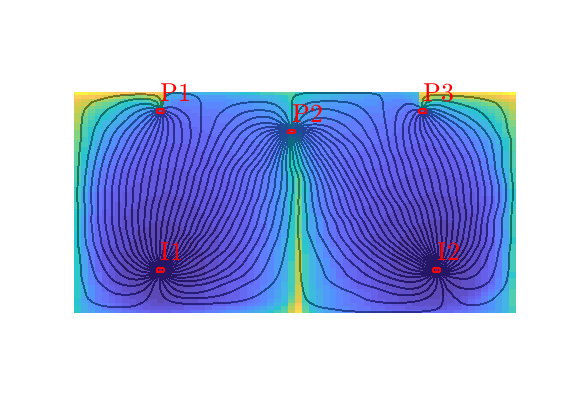
Backward time-of-flight
delete(hd);
hd=plotCellData(G,D.tof(:,2),'EdgeColor','none','FaceAlpha',.6);
% print -dpng diagnost-btof.png;
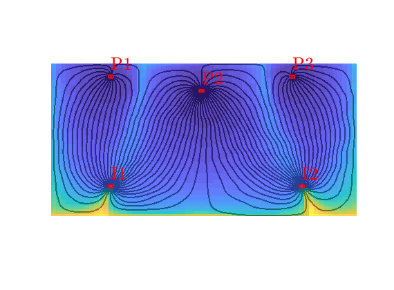
Total travel time/residence time
delete(hd);
hd=plotCellData(G,sum(D.tof,2),'EdgeColor','none','FaceAlpha',.6);
% print -dpng diagnost-ttof.png;
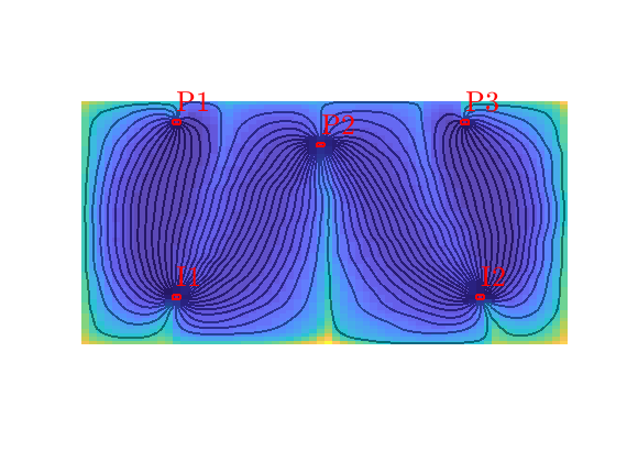
Tracer from I1
delete(hd);
t = D.itracer(:,1);
hd = plotCellData(G, t, t>1e-6, 'EdgeColor','none','FaceAlpha',.6);
% print -dpng diagnost-C-I1.png;
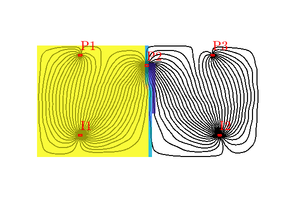
Tracer from P2
delete(hd);
t = D.ptracer(:,2);
hd = plotCellData(G, t, t>1e-6, 'EdgeColor','none','FaceAlpha',.6);
% print -dpng diagnost-C-P2.png;
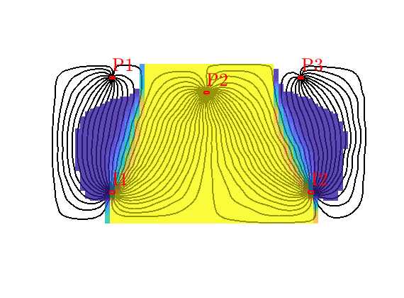
Flooded regions
delete(hd);
hd = plotCellData(G,D.ipart,'EdgeColor','none','FaceAlpha',.6);
% print -dpng diagnost-ipart.png;
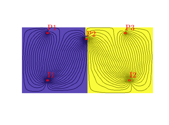
Drainage regions
delete(hd);
hd = plotCellData(G,D.ppart,'EdgeColor','none','FaceAlpha',.6);
% print -dpng diagnost-ppart.png;
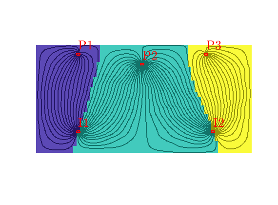
Well regions: I1<->P1, I2<->P3
delete(hd);
hd = plotCellData(G,D.ipart, D.ppart~=2, 'EdgeColor','none','FaceAlpha',.6);
% print -dpng diagnost-wreg.png;
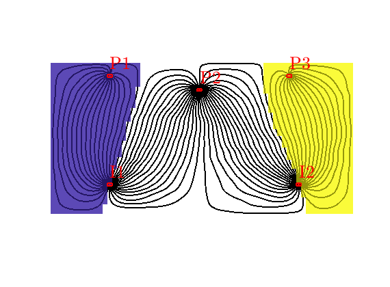
Compute time-of-flights inside each well region
T = computeTimeOfFlight(state, G, rock, 'wells', W, ...
    'tracer',{W(D.inj).cells},'computeWellTOFs', true);
F-Phi diagram
[F,Phi] = computeFandPhi(poreVolume(G,rock), D.tof);
clf,
plot(Phi,F,'.',[0 1],[0 1],'--'); set(gca,'FontSize',20);
% print -depsc2 diagnost-FPhi.eps;
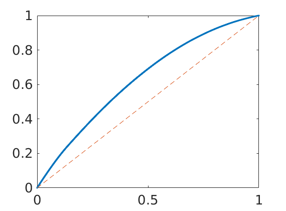
Sweep effciency diagram
[Ev,tD] = computeSweep(F,Phi);
clf
plot(tD,Ev,'.'); set(gca,'FontSize',20);
% print -depsc2 diagnost-sweep.eps;
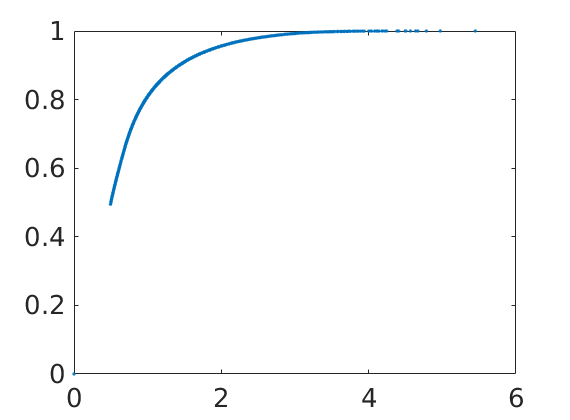
Compute F-Phi per well-pair region
n = 1; cmap=lines;
pv = poreVolume(G,rock);
leg = {};
clf, hold on
for i=1:numel(D.inj),
    for p=1:numel(D.prod)
        I = (D.ipart==i) & (D.ppart==p);
        if sum(I)==0, continue, end;
        [F,Phi] = computeFandPhi(pv(I),D.tof(I,:));
        plot(Phi(1:4:end),F(1:4:end),'.','Color',cmap(n,:));
        n = n+1;
        leg{n} = sprintf('I%d -> P%d', i, p);
    end
end
hold off
legend(leg{:});
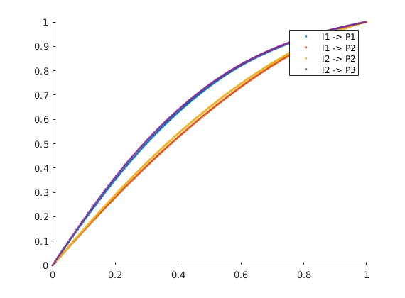
Illustrate the use of residence-time distributions
Generated from showRTD.m
In this example, we compute the residence-time distribution for two different layers of the SPE 10 benchmark test. We compare distributions obtained by tracing a delta pulse through the reservoir and obtained directly from the averaged TOF values.
mrstModule add diagnostics spe10 incomp
Base model
We set up a grid. Later, we will assign petrophysical properties from one single layer at the time
cartDims = [  60,  220,  1];
physDims = [1200, 2200, 2*cartDims(end)] .* ft();
G  = cartGrid(cartDims, physDims);
G  = computeGeometry(G);

% Set fluid model: Here, we use a simple fluid model with properties that
% are typical for water. Replace this by a multiphase fluid object if you
% also want to include fluid effects in the calculation
fluid = initSingleFluid('mu', 1*centi*poise, ...
                        'rho', 1014*kilogram/meter^3);
Compute RTD for a single well
[T,layer] = deal(10*year, [23, 75]);
for n=1:2
    % --- Set petrophysical data for this particular layer
    % To avoid problems with very small porosity values, we explicitly
    % impose a lower threshold of 1e-4
    rock = getSPE10rock(1:cartDims(1),1:cartDims(2),layer(n));
    rock.poro = max(rock.poro, 1e-4);

    % --- Set up well model
    pv  = poreVolume(G, rock);
    W = addWell([], G, rock, 1:60, ...
            'Type', 'rate', 'Val', 3*sum(pv)/T, ...
            'Radius', 0.125, 'Name', 'I', ...
            'InnerProduct', 'ip_tpf', 'Comp_i', 1);
    W = addWell(W, G, rock, (60*219+1):(60*220), ...
            'Type', 'bhp', 'Val', 200*barsa, ...
            'Radius', 0.125, 'Name', 'P', ...
            'InnerProduct', 'ip_tpf', 'Comp_i', 1);

    % --- Initiate and solve flow problem
    rS = initState(G, W, 0, 0.0);
    hT = computeTrans(G, rock);
    rS = incompTPFA(rS, G, hT, fluid, 'wells', W);
    rS.wellSol(1).sign = 1;
    rS.wellSol(2).sign =-1;


    % --- Compute RTD
    D   = computeTOFandTracer(rS, G, rock, 'wells', W, ...
        'maxTOF', inf,'computeWellTOFs', true, 'firstArrival', true);
    WP  = computeWellPairs(rS, G, rock, W, D);
    rtd = computeRTD(rS, G, pv, D, WP, W, 'nsteps',5000);
    RTD = estimateRTD(pv, D, WP);

    % --- Plot RTD
    figure, hold on
    plot(rtd.t/year, rtd.values, '-',  'LineWidth',2);
    plot(RTD.t/year, RTD.values, '--', 'LineWidth',2);
    tfa = min(D.ifa(W(2).cells))/year;      % first arrival
    tm  = RTD.volumes/RTD.allocations/year; % mean time
    vm  = max(RTD.values);
    plot([tfa tfa], [0 vm], ':k', [tm tm], [0 vm], '-k');
    legend('Simulated pulse','From averaged TOF');
    set(gca,'XLim',[0 10],'YLim',[0 5e-8],'FontSize',14);
    xlabel('Time [years]')
    hold off

    axes('Position',[.6 .4 .3 .35]);
    plotCellData(G,log10(rock.perm(:,1)),'EdgeColor','none');
    view(2); axis equal off, colormap(parula)

    % --- F-Phi diagram
    [F, Phi] = computeFandPhi(pv, D.tof);
    [f, phi] = computeFandPhi(rtd, 'sum', true);

    figure
    plot(phi,f, '-', Phi,F, '--', 'LineWidth',2);
    legend(['Simulated pulse: L=',num2str(computeLorenz(f,phi))],...
        ['From averaged TOF: L=', num2str(computeLorenz(F,Phi))], ...
        'Location','SouthEast');
    axis([0 1 0 1]); set(gca,'FontSize',14);
end
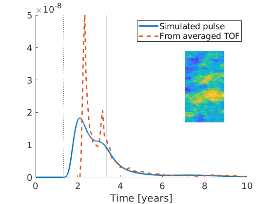
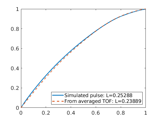
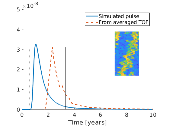
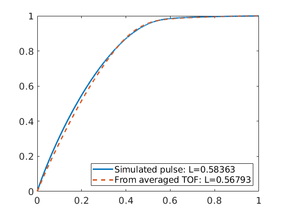
RTD for two well pairs
Set parameters describing the wells
wtype    = {'bhp', 'bhp', 'bhp'};
wtarget  = [200,   200,   600] .* barsa();
wrad     = [0.125, 0.125, 0.125] .* meter;
wloc     = [ 10,   50,    25;
            220,   220,    1];
wname    = {'P1', 'P2', 'I'};
sgn      = [-1 -1 1];

[T,layer] = deal(10*year, [23, 75]);
for n=1:2

    % --- Set petrophysical data for this particular layer
    % To avoid problems with very small porosity values, we explicitly
    % impose a lower threshold of 1e-4
    rock = getSPE10rock(1:cartDims(1),1:cartDims(2),layer(n));
    rock.poro = max(rock.poro, 1e-4);

    % --- Set up well model
    % To ensure that we get the correct well index when updating the
    % petrophysical data, we simply regenerate the well objects.
    W = [];
    for w = 1 : numel(wtype)
       W = verticalWell(W, G, rock, wloc(1,w), wloc(2,w), 1, ...
           'Type', wtype{w}, 'Val', wtarget(w), ...
           'Radius', wrad(w), 'Name', wname{w}, ...
           'InnerProduct', 'ip_tpf', 'Comp_i', 1);
    end

    % --- Initiate and solve flow problem
    pv = poreVolume(G, rock);
    rS = initState(G, W, 0, 0.0);
    hT = computeTrans(G, rock);
    rS = incompTPFA(rS, G, hT, fluid, 'wells', W);
    for i=1:numel(rS.wellSol), rS.wellSol(i).sign = sgn(i); end

    % --- Compute RTD
    D   = computeTOFandTracer(rS, G, rock, 'wells', W, ...
        'maxTOF', inf, 'computeWellTOFs', true, 'firstArrival', true);
    WP  = computeWellPairs(rS, G, rock, W, D);
    rtd = computeRTD(rS, G, pv, D, WP, W, 'nsteps',2500);
    RTD = estimateRTD(pv, D, WP);

    % --- Plot RTD
    figure, hold on
    plot(rtd.t/year, rtd.values, '-', 'LineWidth', 2); set(gca,'ColorOrderIndex',1)
    plot(RTD.t/year, RTD.values, '--', 'LineWidth',2); set(gca,'ColorOrderIndex',1)
    tfa = min(D.ifa(W(2).cells))/year;      % first arrival
    tm  = rtd.volumes./rtd.allocations/year; % mean time
    vm  = max(RTD.values(:));
    plot([1; 1]*tm',repmat([0; vm],1,numel(rtd.volumes)), '-');
    legend('Simulated pulse: P1', 'Simulated pulse: P2', ...
        'From averaged TOF: P1', 'From averaged TOF: P2');
    set(gca,'FontSize',14,'XLim',[0 130]);
    xlabel('Time [years]')
    hold off

    axes('Position',[.6 .3 .3 .35]);
    plotCellData(G,log10(rock.perm(:,1)),'EdgeColor','none');
    outlineCoarseGrid(G,D.ppart,'LineWidth',1);
    view(2); axis equal off, colormap(parula)
    x = G.cells.centroids(vertcat(W.cells),:);
    hold on
    plot(x(:,1),x(:,2),'ok','MarkerSize',8,'MarkerFaceColor','w');
    text(x(:,1)+40,x(:,2), {W.name});
    hold off

    % --- F-Phi diagram
    [f, phi ] = computeFandPhi(rtd);
    [tf,tphi] = computeFandPhi(rtd, 'sum', true);

    figure, hold on
    plot(phi,f, '-', tphi, tf, '-','LineWidth',2);
    legend('Simulated pulse: P1', 'Simulated pulse: P2', ...
        'Simulated pulse: whole field','Location','SouthEast');
    hold off
    axis([0 1 0 1]); set(gca,'FontSize',14);
end
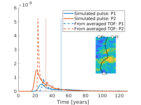
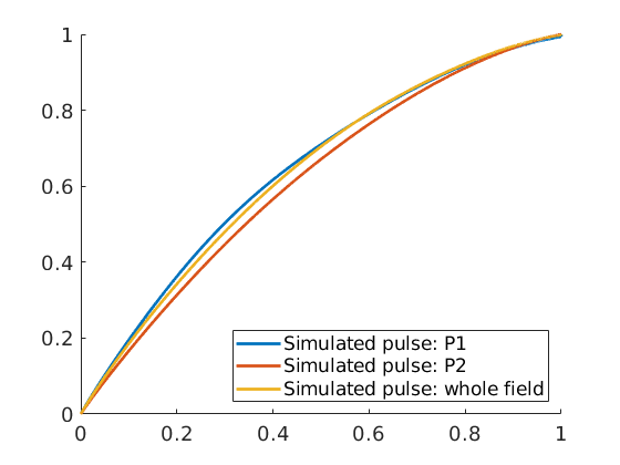
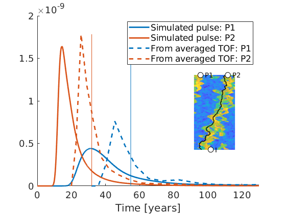
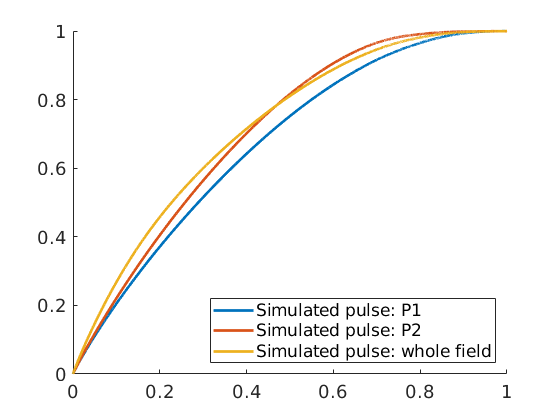
Generate Coarse Grids with Near-Well Refinement
Generated from coarsenCaseB4.m
Pressure gradients and flow rates will typically be much larger near wells than inside the reservoir. The accuracy with which we represent the flow in and out of wells will to a large extent determine the accuracy of an overall simulation and as a result one therefore often desires to have higher grid resolution in the near-well zone than inside the reservoir. The example considers the smallest pillar grid from CaseB4, which can either be partitioned rectangularly in index space, or using METIS with transmissibilities as edge weights. The latter approach gives blocks with boundaries aligning to sharp media contrasts. On top of this, we split partitions across faults and use the function ‘refineNearWell’ to impose radial refinement in near-well regions.
mrstModule add coarsegrid incomp
useMetis = false;
Load grid model and create petrophysical data
file = fullfile(getDatasetPath('CaseB4'),'pillar_36x48.grdecl');
G = processGRDECL(readGRDECL(file));
G = computeGeometry(G);
layers = [1 2 8 12 13];
K = logNormLayers(G.cartDims, [50 300 100 20]*milli*darcy, ...
                  'sz', [51 3 3], 'indices', layers);
rock = makeRock(G, bsxfun(@times, K*milli*darcy,[1 1 .1]), 0.2);

W = verticalWell([], G, rock, G.cartDims(1), 1, [], 'InnerProduct', 'ip_tpf');
W = verticalWell(W, G, rock, 14, 36, [],'InnerProduct', 'ip_tpf');

clf
plotCellData(G, log10(rock.perm(:,1)),'EdgeAlpha',.1); view(3);
plotWell(G, W, 'height', 30,'FontSize',12);
colormap(jet), axis tight off, view(250, 50)
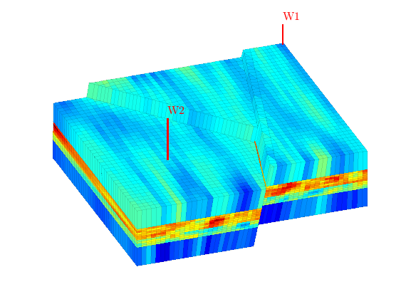
Uniform/METIS partition
We consider two possible partitions. The first is a standard load-balanced partition in index space. The second is an unstructured partitioning by the METIS graph library that adapts to the underlying geology. To this end, we transmissibilities as edge-weights in the graph-partitioning algorithm of METIS so that it tries to make grid blocks having as homogeneous permeability as possible.
if useMetis
    hT = computeTrans(G, rock);
    p0 = partitionMETIS(G, hT, 7*9*4, 'useLog', true);
else
    p0 = partitionUI(G, [7 9 1]); max(p0)
end
figure, myPlotPartition(G, W, p0, 400);
ans =

    63
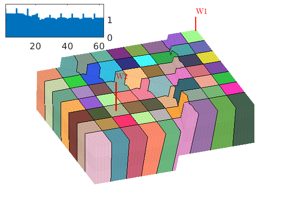
Split fault faces
It may also be advantageous to split blocks across faults, even if this will introduce some very small blocks
if useMetis
    % hT(G.faces.tag==1) = 1e-10*min(hT);
    % pf = partitionMETIS(G, hT, 7*9*4, 'useLog', true, 'ufactor',5);
    pf = p0;
else
    pf = processPartition(G, p0, find(G.faces.tag==1)); max(pf)
end
figure, myPlotPartition(G, W, pf, 400);
ans =

    79

Radial refinement
The function ‘refineNearWell’ takes a set of points and partitions these according to the distance in the xy-plane from a single well point. Here, we will this function to refine the coarse blocks that contains wells. The first well is placed in the corner and we partition the perforated well block into five radial sections. The width of the radial sections is set to decay as log(r). For the second well, we refine all the neighboring blocks surrounding the well block using a number of angular sectors that increases as we move radially out from the well point.
angSectors = {1, [1,4,6,9]};
radSectors = [4 4];
pw = pf;
for i=1:numel(W)
    wc    = W(i).cells(1);
    wpt   = G.cells.centroids(wc,:);
    pwv   = pw(wc);
    if i==1
        % Pick all cells inside the well block
        cells = (pw==pwv);
    else
        % Use adjacency matrix to compute nearest neighbors. We start with
        % a vector e which is equal one in the well block and zero
        % elsewhere. Multiplying by the adjacency matrix A will set the
        % value in each block equal the sum over the block and its
        % face-neighbors. After two multiplications, all blocks surrounding
        % the initial block should have value larger than one.
        CG    = generateCoarseGrid(G, pw);
        A     = getConnectivityMatrix(getNeighbourship(CG),true,CG.cells.num);
        rblk  = zeros(CG.cells.num,1); rblk(pwv)=1; rblk((A*A*rblk)>1) = 1;
        cells = rblk(pw)>0;
    end
    pts   = G.cells.centroids(cells,:);
    out   = refineNearWell(pts, wpt, 'angleBins', angSectors{i}, ...
        'radiusBins', radSectors(i), 'logbins', true, 'maxRadius', inf);
    pw(cells) = max(pw) + out;
end
pw = compressPartition(pw);
figure, myPlotPartition(G, W, pw, 400);
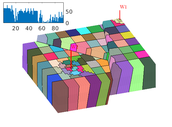
Refine partition in the vertical direction
For the Cartesian partition, we end by refining the partition in the vertical direction so that it follows the layering in the petrophysical data, which we assume is known.
if ~useMetis
    pK = rldecode((1:numel(layers)-1)',diff(layers));
    [~,~,k]=gridLogicalIndices(G);
    pk = compressPartition((pK(k)-1)*max(pw)+pw);
    pk = processPartition(G, pk);
    figure, myPlotPartition(G, W, pk, 400);
end
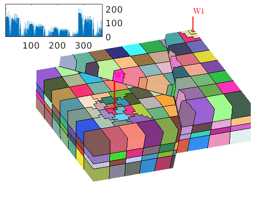
Coarsen Real Models: the Johansen Formation
Generated from coarsenJohansen.m
In this script we will look at how to coarsen real model: a sector model of the Johansen aquifer which was considered as a possible candidate for large-scale geological storage of CO2. The data can be downloaded from http://www.sintef.no/Projectweb/MatMorA/Downloads/Johansen/
mrstModule add coarsegrid;

dpath = getDatasetPath('johansen');
sector = fullfile(dpath, 'NPD5');
filename = [sector, '.grdecl'];
G = processGRDECL(readGRDECL(filename));
G = computeGeometry(G);
K = reshape(load([sector, '_Permeability.txt'])', prod(G.cartDims), []);
K = K(G.cells.indexMap);
First, we make a partition with a coarsening factor four in each lateral direction. In the vertical direction, the model consists of three different formations that can be distinguised by the permeability values: the Dunlin shale has K<=0.01mD, the Amundsen shale has K<0.1mD, whereas the Johansen sandstone has K>1mD. For illustration purposes, we only keep one block in the vertical direction for each of the formations.
pK = 2*ones(size(K));  % Johansen
pK(K<=0.1) = 3;        % Amundsen
pK(K<=0.01)= 1;        % Dunlin
pC = partitionUI(G, [G.cartDims(1:2)/4 1]);
[~,~,p] = unique([pK, pC], 'rows');
p = processPartition(G,p);

clf
plotCellData(G,log10(K),'EdgeColor','k','EdgeAlpha',.4); view(3)
outlineCoarseGrid(G,p,'FaceColor','none','EdgeColor','k','LineWidth',1.5);
axis tight off
colormap((2*jet(16)+ones(16,3))/3);
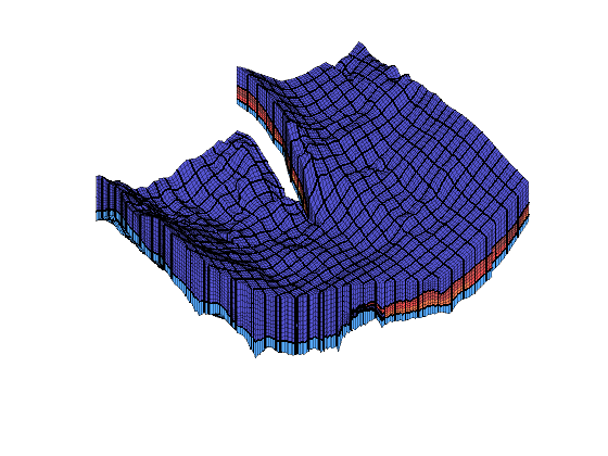
Make a new coarse grid in which we keep the vertical resolution, which is typically what one would do if the model is to be used to simulate CO2 storage. The resulting coarse model will have many coarse blocks that have more than six connections. We loop through the blocks in the top layer to show how they look like
pK = 2*ones(size(K)); pK(K<=0.1) = 3; pK(K<=0.01)= 1;
pC = partitionUI(G, G.cartDims./[4 4 1]);
[~,~,p] = unique([pK, pC], 'rows');
p = processPartition(G,p);
CG = generateCoarseGrid(G,p);
cn = diff(CG.cells.facePos);

figure('Position',[0 60 560 820])
subplot(2,1,1);
plotGrid(G,'FaceColor','none','EdgeAlpha',.1);
plotGrid(CG,cn>6);

h1=[];
val = cumsum(ones(G.cartDims),3); val=val(G.cells.indexMap);
kn = zeros(size(cn)); kn(p) = val;
ind = find(cn>6 & kn==1);
for i=1:numel(ind)
   subplot(2,1,1); delete(h1);
   h1 = plotGrid(CG,ind(i),'FaceColor','r');

   subplot(2,1,2); cla;
   plotGrid(G,p==ind(i));
   plotGrid(CG,ind(i),'FaceColor','none','LineWidth',2);
   title(['Block number: ' num2str(ind(i))]);
   view(3); drawnow;

end
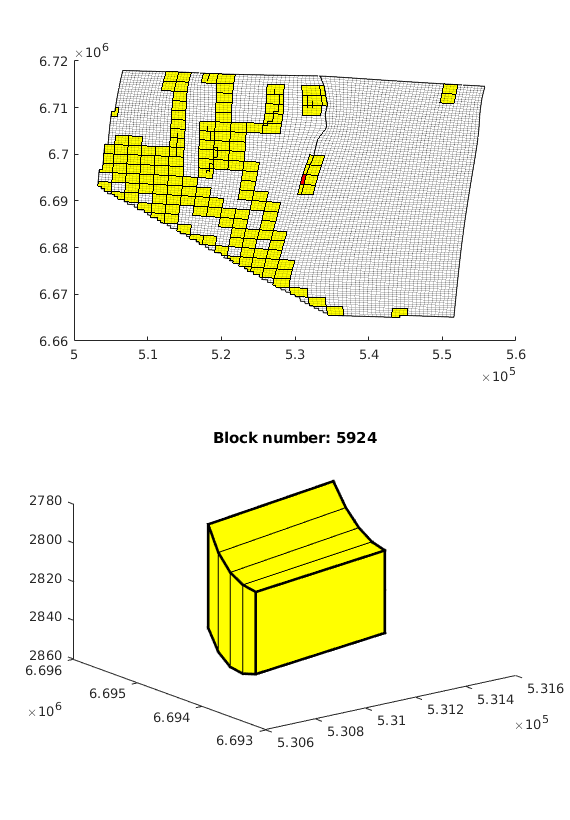
lock = [89 139 143 195 286 466];
ind = [1 5:8 4];
c   = colorcube(9);
col = (2*c(1:6,:)+ones(6,3))/3;
figure('position',[0 60 1000 400]);
subplot(2,4,2:3)
plotGrid(G,'FaceColor','none','EdgeAlpha',.1);
axis off; zoom(1.3);
for i=1:6
   subplot(2,4,2:3);
   plotGrid(CG,block(i),'FaceColor',col(i,:));
   subplot(2,4,ind(i));
   plotGrid(G,p==block(i),'FaceColor',col(i,:));
   plotGrid(CG,block(i),'FaceColor','none','LineWidth',2);
   view(3); set(gca,'Clipping','off'), axis tight off
   zoom(1.3)
end
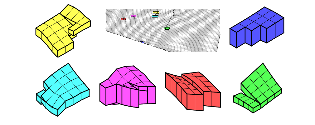
Coarsen Real Models: SAIGUP Shallow-Marine Reservoir Model
Generated from coarsenSAIGUP.m
The <http://www.fault-analysis-group.ucd.ie/Projects/SAIGUP.html>SAIGUP project is a systematic assessment of uncertainty in reserves and production estimates within an objectively defined geological parameterisation encompassing the majority of European clastic oil reservoirs. A broad suite of shallow marine sedimentological reservoir types are indexed to continuously varying 3D anisotropy and heterogeneity levels. Structural complexity ranges from unfaulted to compartmentalised, and fault types from transmissive to sealing. Several geostatistical realisations each for the geologically diverse reservoir types covering the pre-defined parameter-space are up-scaled, faulted and simulated with an appropriate production strategy for an approximately 20 year period. Herein, we will inspect in detail one instance of the model, which can be downloaded from the <http://www.sintef.no/Projectweb/MRST>MRST webpage
Load dataset
mrstModule add libgeometry coarsegrid
filename = fullfile(getDatasetPath('SAIGUP'), 'SAIGUP.GRDECL');
G = processGRDECL(readGRDECL(filename));
try
   G = mcomputeGeometry(G);
catch %#ok<CTCH>
   G = computeGeometry(G);
end
We construct a coarse grid by partitioning the grid uniformly as 6x12x3 coarse blocks in index space. This process partitions all cells in the logical 40x120x20 grid, including cells that are inactive. We therefore compress the partitioning to remove blocks that contain no active cells, and then renumber the overall partitioning. Some of the blocks may contain disconnected cells because of erosion, faults, etc. We therefore postprocess the grid in physical space and split disconnected blocks.
p = partitionUI(G,[6 12 3]);
p = compressPartition(p);
p = processPartition(G,p);
We have now obtained a partitioning consisting of 243 blocks, in which each coarse block consists of a set of connected cells in the fine grid. To show the partition, we plot the coarse blocks using the explosion view technique
figure('Position',[0 60 800 420]);
axes('Position',[.01 .11 .775 .81]);
explosionView(G, p, 'EdgeAlpha', .1);
axis tight off; set(gca,'DataAspect',[1 1 0.1]);
view(-65,55); zoom(1.4); camdolly(0,-0.2,0)
colormap(.3*(2*colorcube(max(p))+ones(max(p),3)));
set(gca,'Clipping','off')

Build the coarse-grid and inspect the distribution of block volumes. The original fine-scale model has the peculiar characteristic that all cells have the same size. In the coarsened model there is almost two orders difference between the smallest and largest blocks.
CG = generateCoarseGrid(G, p); P=p;
CG = coarsenGeometry(CG);
axes('Position',[.75 .12 .18 .8]);
h = barh(CG.cells.volumes,'b');
set(gca,'xdir','reverse','YAxisLocation','right',...
'Fontsize',8,'XLim',[0 12]*1e6);
set(h,'FaceColor',[.7 .7 .7],'EdgeColor',[.6 .6 .6]);
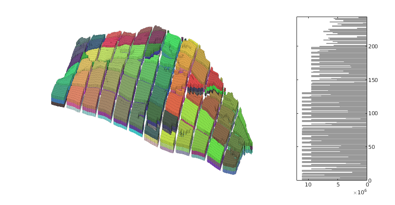
To get a more even size distribution for the coarse blocks, we will remove some of the smallest blocks by merging them with the neighbor that has the smallest block volume. This is done repeatedly until the volumes of all blocks are above a certain lower threshold. First, we visualize all blocks that have volume less than ten percent of the mean block volume.
blockVols = CG.cells.volumes;
meanVol = mean(blockVols);
show = blockVols<.1*meanVol;
figure
plotGrid(G,'FaceColor','none','EdgeAlpha',.05);
bcol = zeros(max(p),1); bcol(show)=1:sum(show);
plotCellData(CG,bcol, show);
axis tight off; set(gca,'DataAspect',[1 1 0.1]);
view(-65,55); zoom(1.4); camdolly(0,-0.2,0)
colormap(lines);
set(gca,'Clipping','off')
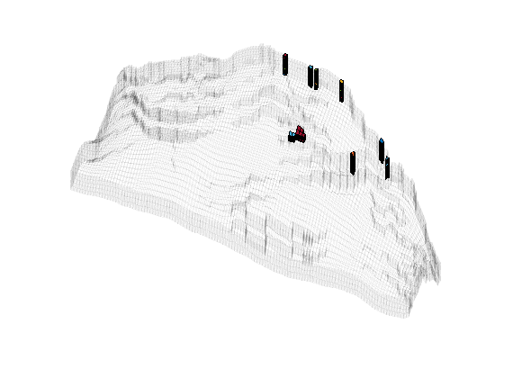
The merging algorithm is quite simple: we compute the block volumes, select the block with the smallest volume, and then merge this block with one of its neighbors, depending on some criterion (e.g., the neighbor with the largest or smallest block volume). Then we update the partition vector by relabling all cells in the block with the new block number, compress the partition vector to get rid of empty entries, regenerate a coarse grid, recompute block volumes, pick the block with the smallest volume in the new grid, and so on. In each iteration, we plot the selected block and its neighbors.
blockVols = CG.cells.volumes;
meanVol = mean(blockVols);
[minVol, block] = min(blockVols);
while minVol<.1*meanVol
% Find all neighbors of the block
clist = any(CG.faces.neighbors==block,2);
nlist = reshape(CG.faces.neighbors(clist,:),[],1);
nlist = unique(nlist(nlist>0 & nlist~=block));
% Alt 1: merge with neighbor having smallest volume
% [~,merge] = min(blockVols(nlist));
% Alt 2: sort neigbors by cell volume and merge with the one in the
% middle
% [~,ind] = sort(blockVols(nlist),1,'descend');
% merge = ind(round(numel(ind)/2));
% Alt 3: merge with neighbor having largest volume
[~,merge] = max(blockVols(nlist));
figure;
plotBlockAndNeighbors(CG, block, ...
'PlotFaults', [false, true], 'Alpha', [1 .8 .8 .8]);
% Update partition vector
p(p==block) = nlist(merge);
p = compressPartition(p);
% Regenerate coarse grid and pick the block with the smallest volume
CG = generateCoarseGrid(G, p);
CG = coarsenGeometry(CG);
blockVols = CG.cells.volumes;
[minVol, block] = min(blockVols);
end
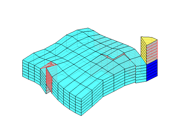
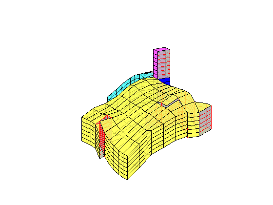
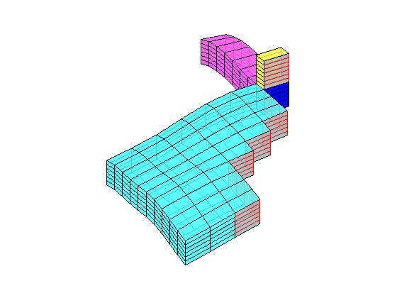
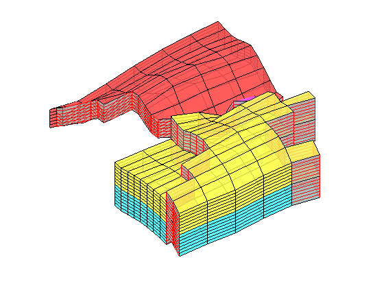
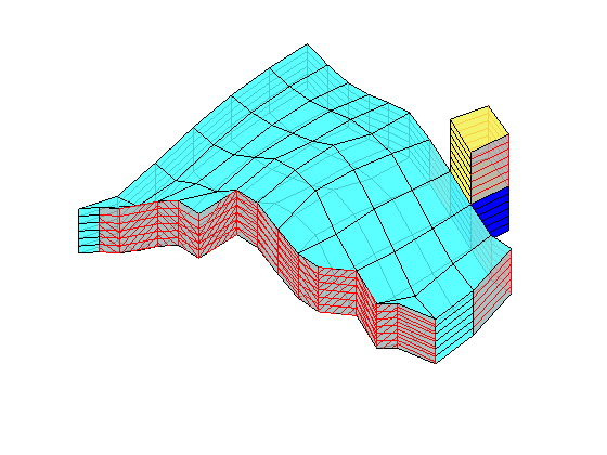
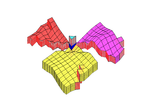
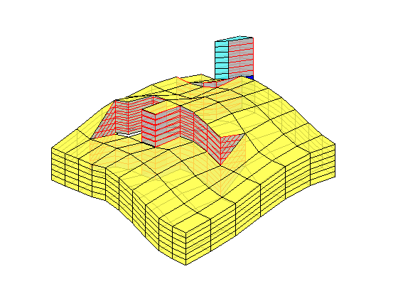
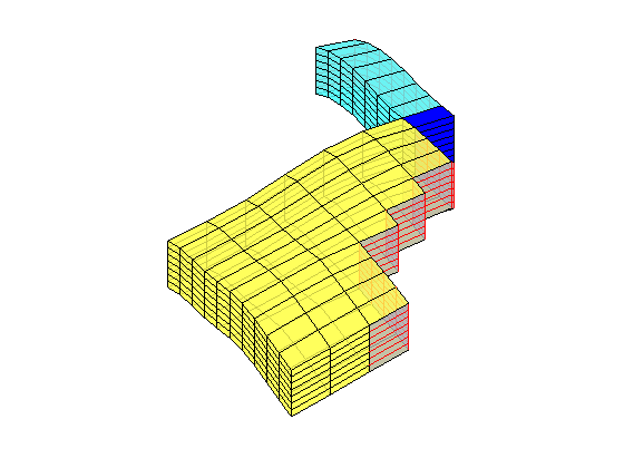
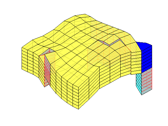
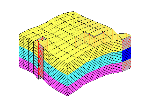
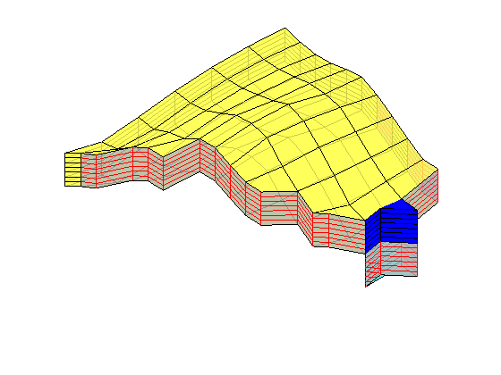
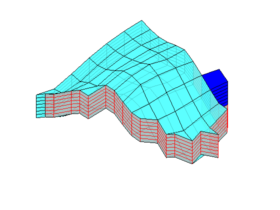
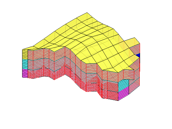
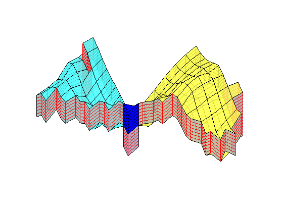
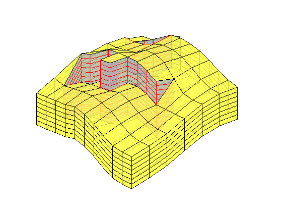
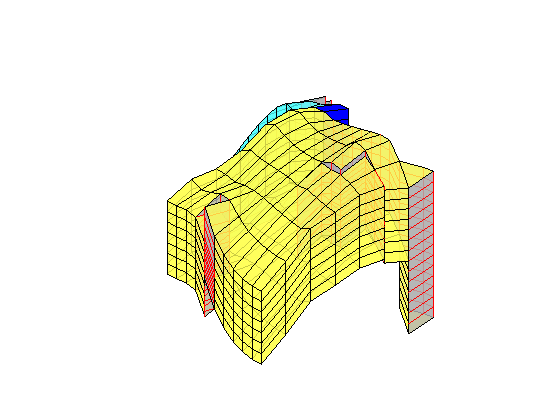
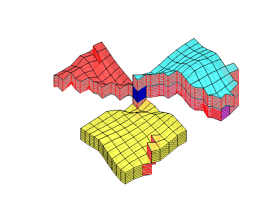
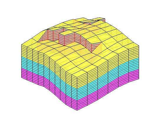
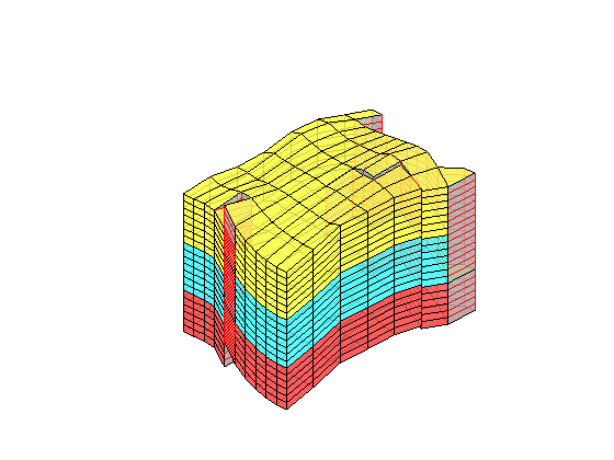
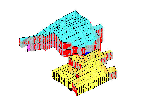
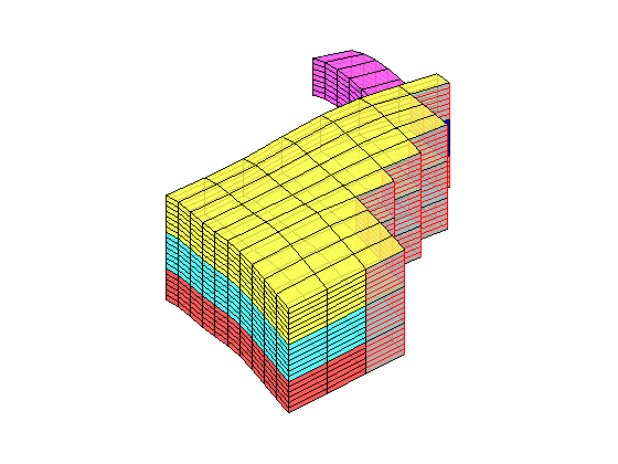
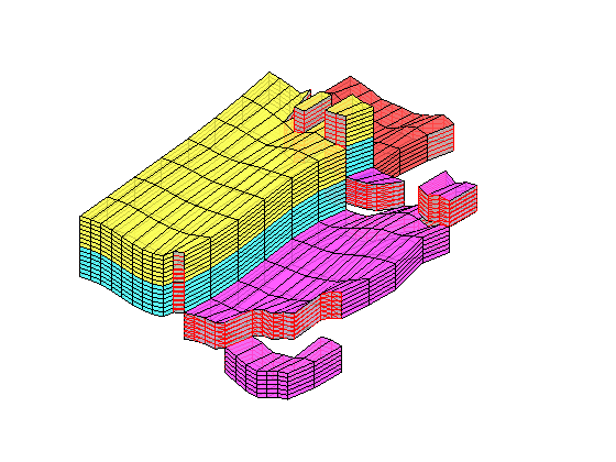
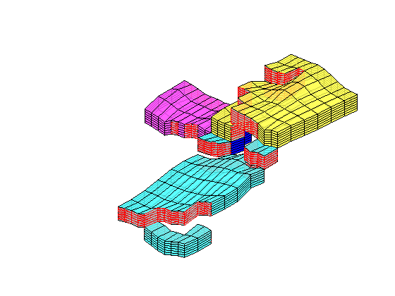
Make new plot with the revised coarse grid
figure('Position',[0 60 800 420]);
axes('Position',[.01 .11 .775 .81]);
explosionView(G, CG.partition, 'EdgeAlpha', .1);
axis tight off; set(gca,'DataAspect',[1 1 0.1]);
view(-65,55); zoom(1.4); camdolly(0,-0.2,0)
colormap(.3*(2*colorcube(CG.cells.num)+ones(CG.cells.num,3)));
set(gca,'Clipping','off')
axes('Position',[.75 .12 .18 .8]);
h = barh(CG.cells.volumes,'b');
set(gca,'xdir','reverse','YAxisLocation','right',...
'Fontsize',8,'XLim',[0 12]*1e6);
set(h,'FaceColor',[.7 .7 .7],'EdgeColor',[.6 .6 .6]);
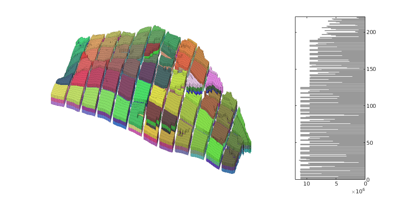
In the partition above, there were several blocks that were only connected through small face areas in their interior. To try to improve this problem, we recompute the the partitioning, but now disregard couplings across small faces when postprocessing the initial, uniform partition
p = partitionUI(G,[6 12 3]);
p = compressPartition(p);
p = processPartition(G, p, G.faces.areas<250);
CG1 = generateCoarseGrid(G,p);
CG1 = coarsenGeometry(CG1);
The next step is to redo the merging of small blocks. The algorithm used above was written to make the visualization of the changing grid as simple as possible. The implementation is not very efficient since we in each step regenerate the coarse grid and compute all the block volumes. This time, we will use another implementation that is a bit more involved, but also more efficient.
blockVols = CG1.cells.volumes;
meanVol = mean(blockVols);
newBlockList = 1:max(p);
[minVol, block] = min(blockVols);
while minVol<.1*meanVol
nlist = reshape(CG1.faces.neighbors(any(CG1.faces.neighbors==block,2),:),[],1);
nlist = newBlockList(nlist(nlist>0));
nlist = unique(nlist(nlist~=block));
[nVol,merge] = min(blockVols(nlist));
newBlockNo = nlist(merge);
p(p==block) = newBlockNo;
newBlockList(block) = newBlockNo;
blockVols(block) = inf;
blockVols(newBlockNo) = minVol + nVol;
[minVol, block] = min(blockVols);
end
p = compressPartition(p);
CG1 = generateCoarseGrid(G, p);
CG1 = coarsenGeometry(CG1);
Make new plot with the revised coarse grid
igure('Position',[0 60 800 420]);
axes('Position',[.01 .11 .775 .81]);
explosionView(G, CG1.partition, 'EdgeAlpha', .1);
axis tight off; set(gca,'DataAspect',[1 1 0.1]);
view(-65,55); zoom(1.4); camdolly(0,-0.2,0)
colormap(.3*(2*colorcube(CG1.cells.num)+ones(CG1.cells.num,3)));
set(gca,'Clipping','off')
axes('Position',[.75 .12 .18 .8]);
h = barh(CG1.cells.volumes,'b');
set(gca,'xdir','reverse','YAxisLocation','right',...
'Fontsize',8,'XLim',[0 12]*1e6);
set(h,'FaceColor',[.7 .7 .7],'EdgeColor',[.6 .6 .6]);
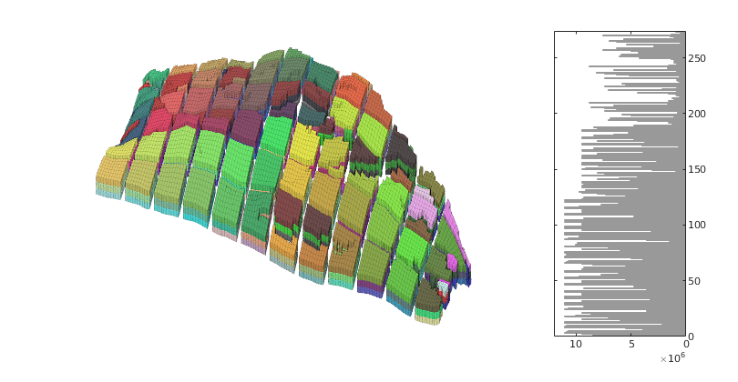
Example: three uses of simpleGrdecl
Generated from exampleGrids.m
grdecl = simpleGrdecl([20, 20, 5]);
G = processGRDECL(grdecl);
clf, plotGrid(G,'FaceColor',[.8 .8 .8]), view(3), axis tight off
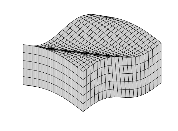
grdecl = simpleGrdecl([20, 20, 5], @(x) 0.05 * (sin(2*pi*x) - 1.5));
G = processGRDECL(grdecl);
clf, plotGrid(G,'FaceColor',[.8 .8 .8]), view(3), axis tight off
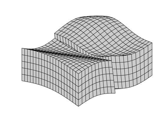
grdecl = simpleGrdecl([20, 20, 5], @(x) 0.25*(x-0.5), 'flat', true);
G = processGRDECL(grdecl);
clf, plotGrid(G,'FaceColor',[.8 .8 .8]), view(3), axis tight off
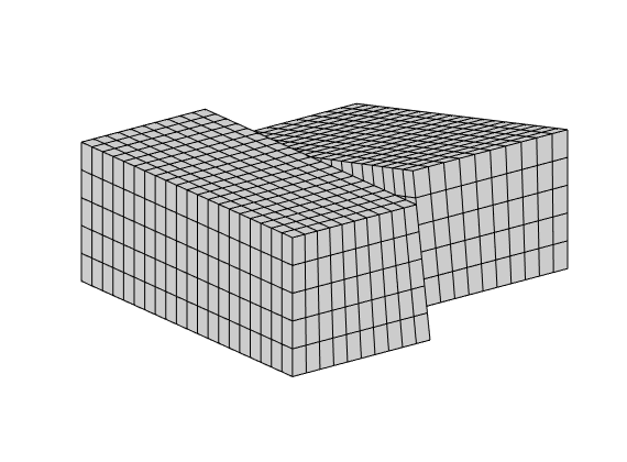
Example: makeModel3
grdecl = makeModel3([30,20,5]);
G = processGRDECL(grdecl);
clf, plotGrid(G,'FaceColor',[.8 .8 .8]), view(130,30), axis tight off
plotFaces(G,find(G.faces.tag>0),'FaceColor',[.6 .6 .6]);
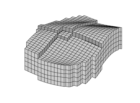
Example: extrudedTriangleGrid
G = extrudedTriangleGrid(50);
clf, plotGrid(G,'FaceColor',[.8 .8 .8]), view(-30,60), axis tight off
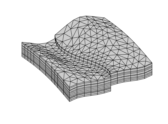
= extrudedTriangleGrid(50, true);
clf, plotGrid(G,'FaceColor',[.8 .8 .8]), view(-30,60), axis tight off
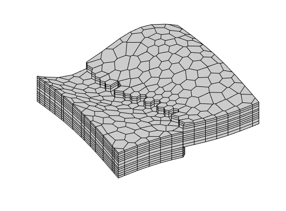
mrstModule add agglom coarsegrid diagnostics incomp spe10
CaseB4: merge small cells
Generated from showAgglomExamples.m
Load and set up model
file = fullfile(getDatasetPath('CaseB4'),'pillar_36x48.grdecl');
G = processGRDECL(readGRDECL(file));
G = computeGeometry(G);
layers = [1 2 8 12 13];
K = logNormLayers(G.cartDims, [50 300 100 20]*milli*darcy, ...
'sz', [51 3 3], 'indices', layers);
rock = makeRock(G, bsxfun(@times, K*milli*darcy,[1 1 .1]), 0.2);
W = verticalWell([], G, rock, G.cartDims(1), 1, [], 'InnerProduct', 'ip_tpf');
W = verticalWell(W, G, rock, 14, 36, [],'InnerProduct', 'ip_tpf');
% Partition topology and split across faults
p0 = partitionUI(G, [7 9 1]);
pf = processPartition(G, p0, find(G.faces.tag==1));
figure, myPlotPartition(G, W, pf, 400);
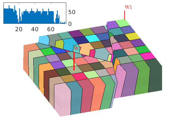
Merge small blocks To avoid merging across faults, we generate a static partition that splits the model into three different fault blocks
I = poreVolume(G, rock)./G.cells.volumes;
pm = mergeBlocks(pf, G, I, I, 50, 'static_partition', ...
processPartition(G,ones(G.cells.num,1),find(G.faces.tag==1)));
figure, myPlotPartition(G, W, pm, 400);
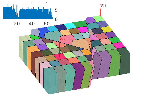
Adaptive Cartesian coarsening for layer of SPE10
We consider a subset of layer 25 from SPE 10 and study how recursive Cartesian refinement works for three different indicator functions: permeability, velocity, and time of flight.
% Setup model
[G, W, rock] = getSPE10setup(25);
for i = 1:numel(W), W(i).compi = 1; end
rock.poro = max(rock.poro, 1e-4);
fluid = initSingleFluid('mu', 1*centi*poise, 'rho', 1014*kilogram/meter^3);
hT = computeTrans(G, rock);
rS = incompTPFA(initState(G,W,0), G, hT, fluid, 'wells', W);
Tf = computeTimeOfFlight(rS, G, rock, 'wells', W);
Tb = computeTimeOfFlight(rS, G, rock, 'wells', W, 'reverse', true);
pv = poreVolume(G, rock);
% Construct indicators
iK = log10(rock.perm(:,1)); iK = iK - min(iK) + 1;
v = sqrt(sum(faceFlux2cellVelocity(G, rS.flux).^2, 2));
iV = log10(v); iV = iV - min(iV) + 1;
iT = -log10(Tf+Tb); iT = iT - min(iT) + 1;
% Extract subset of model
p1 = partitionUI(G, [3, 11, 1]);
ind = find(p1<19);
G = extractSubgrid(G, ind);
[p1,iK,iV,iT,pv] = deal(p1(ind),iK(ind),iV(ind),iT(ind),pv(ind));
% Recursively subdivide the blocks by a factor 2x2
pK = refineUniformShape(p1, G, iK, 25, 'CartDims', [2,2,1]);
pV = refineUniformShape(p1, G, iV, 25, 'CartDims', [2,2,1]);
pT = refineUniformShape(p1, G, iT, 25, 'CartDims', [2,2,1]);
% Plot the results
I = {iK, iV, iT}; p = {pK, pV, pT};
head = {'Permeability', 'Velocity', 'Time-of-flight'};
wc = vertcat(W.cells);
x = G.cells.centroids(wc(wc<G.cells.num),:);
clf; set(gcf,'Position',[510 420 850 400]);
for i=1:3
subplot(1,3,i)
plotCellData(G,I{i},'EdgeColor','none');
hold on
plot(x(:,1),x(:,2),'ok','MarkerSize',7,'MarkerFaceColor','w'); hold off
outlineCoarseGrid(G, p{i}, 'EdgeColor','k'); axis tight off
title([head{i} ' indicator']);
end
colormap(jet(128)*.7+.3*ones(128,3));
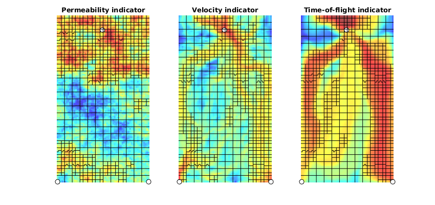
Non-uniform coarsening
We outline the main steps of the original NUC algorithm proposed by Aarnes et al. To this end, we extract a further subdivision of the model
ind = find(p1>9);
G = extractSubgrid(G, ind);
[p1,iK,iV,iT,pv] = deal(p1(ind),iK(ind),iV(ind),iT(ind),pv(ind));
volI = pv./G.cells.volumes;
flwI = iV;
clf,set(gcf,'Position',[50 560 1400 240]);
subplot(1,6,1)
plotCellData(G, flwI, 'EdgeColor','none'); axis tight
set(gca,'XTick',[],'YTick',[]); title('Indicator');
subplot(1,6,2)
ps = segmentIndicator(G, flwI, 5);
plotCellData(G, ps, 'EdgeColor','none'); axis tight
outlineCoarseGrid(G, ps, 'EdgeColor','k','FaceColor','none');
set(gca,'XTick',[],'YTick',[]); title('segmentIndicator');
xlabel(['#blocks: ' num2str(max(ps))]);
subplot(1,6,3)
pm1 = mergeBlocks(ps, G, volI, flwI, 20);
plotCellData(G, pm1, 'EdgeColor','none'); axis tight
outlineCoarseGrid(G, pm1, 'EdgeColor','k','FaceColor','none');
set(gca,'XTick',[],'YTick',[]); title('mergeBlocks');
xlabel(['#blocks: ' num2str(max(pm1))]);
subplot(1,6,4)
pr = refineGreedy(pm1, G, flwI, 30);
plotCellData(G, pr, 'EdgeColor','none'); axis tight
outlineCoarseGrid(G, pr, 'EdgeColor','k','FaceColor','none');
set(gca,'XTick',[],'YTick',[]); title('refineGreedy');
xlabel(['#blocks: ' num2str(max(pr))]);
subplot(1,6,5)
pm2 = mergeBlocks(pr, G, volI, flwI, 20);
plotCellData(G, pm2, 'EdgeColor','none'); axis tight
outlineCoarseGrid(G, pm2, 'EdgeColor','k','FaceColor','none');
set(gca,'XTick',[],'YTick',[]); title('mergeBlocks');
xlabel(['#blocks: ' num2str(max(pm2))]);
subplot(1,6,6);
p = mergeBlocks2(ps, G, volI, flwI, 20, 30);
p = refineGreedy2(p, G, flwI, 30, 'nlevel',1);
p = mergeBlocks2(p, G, volI, flwI, 20, 30);
plotCellData(G, p, 'EdgeColor','none'); axis tight
outlineCoarseGrid(G, p, 'EdgeColor','k','FaceColor','none');
set(gca,'XTick',[],'YTick',[]); title('Version 2');
xlabel(['#blocks: ' num2str(max(p))]);
colormap(jet(128)*.6+.4*ones(128,3));
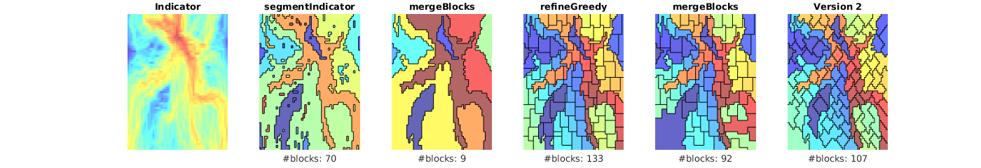
mrstModule add agglom coarsegrid
—— S E G M E N T A T I O N ——
Generated from showAgglomModule.m
Demonstrate segmentation: apply to CaseB4 model
rng(1,'twister'); % reset random generator to reproduce the same results
file = fullfile(getDatasetPath('CaseB4'),'pillar_36x48.grdecl');
G = processGRDECL(readGRDECL(file));
G = computeGeometry(G);
layers = [1 2 8 12 13];
K = logNormLayers(G.cartDims, [50 300 150 20],'sz', [51 3 3], 'indices', layers);
Plot permeability and outline initial bins We segment the permeability, but only out put the initial bins without splitting disconnected components
p = segmentIndicator(G, K, [0 30 80 205 inf],'split',false);
figure(1); clf
plotCellData(G, K,'EdgeAlpha',.1);
view(-120,15), axis tight, set(gca,'Projection','Perspective');
colormap(.8*jet+0.2*ones(size(jet)));
[~, hh]=colorbarHist(K, [0 450], 'South', 100);
h = outlineCoarseGrid(G,p,'EdgeColor','k','LineWidth',2,'FaceColor','none');
hold(hh,'on');
ym = .8*max(reshape(get(get(hh,'Children'),'YData'),[],1));
plot(hh,[30 80 205; 30 80 205], [0 0 0; ym ym ym],'Color',[.3 .3 .3],'LineWidth',2);
hold(hh,'off'); axis off
%set(hc,'FontSize',16);
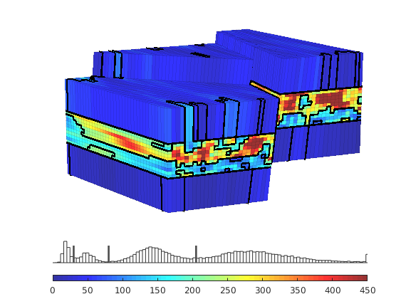
Plot bins resulting from the segmentation
figure(2); clf
plotCellData(G, p,'EdgeAlpha',.1);
mp = max(p);
caxis([.5 mp+.5]); colormap(.8*tatarizeMap(mp)+.2*ones(mp,3));
view(-120,15), axis tight off, set(gca,'Projection','Perspective');
[hc,hh] = colorbarHist(p, [.5 mp+.5], 'South', mp);
bar(hh,accumarray(p,1),'FaceColor','none');
set(hh,'XLim',[.5 mp+.5]);
axis(hh,'off');
set(hc,'XTick',1:4); % set(hc,'FontSize',16);
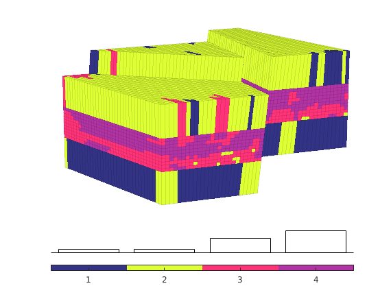
—– S A N I T Y C H E C K S ——
Split connected components (done by initial segmentation)
p = segmentIndicator(G, K, [0 30 80 205 inf]);
figure(1); clf
plotCellData(G, p,'EdgeAlpha',.1);
mp = max(p);
caxis([.5 mp+.5]); colormap(.8*tatarizeMap(mp)+.2*ones(mp,3));
view(-120,15), axis tight off, set(gca,'Projection','Perspective');
[hc,hh] = colorbarHist(p, [.5 mp+.5], 'South', mp);
bar(hh,log10(accumarray(p,1)),'FaceColor','none');
set(hh,'XLim',[.5 mp+.5]);
axis(hh,'off');
set(hc,'FontSize',16);
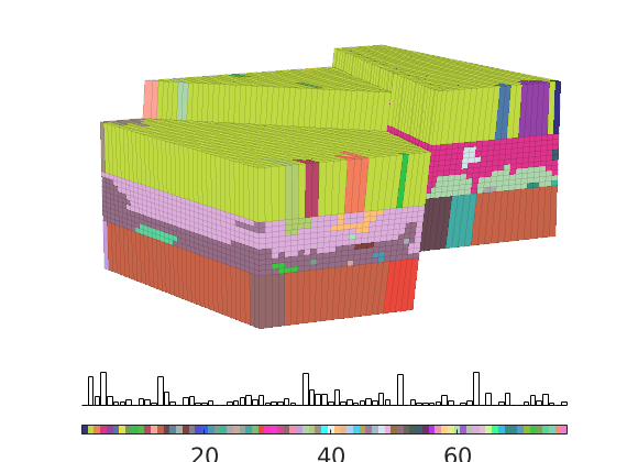
Detect confined blocks
cb = findConfinedBlocks(G, p);
flag=false(mp,1); flag(cb)=true;
plotGrid(G,flag(p),'FaceColor','k','EdgeColor','k');
delete([hc,hh]);
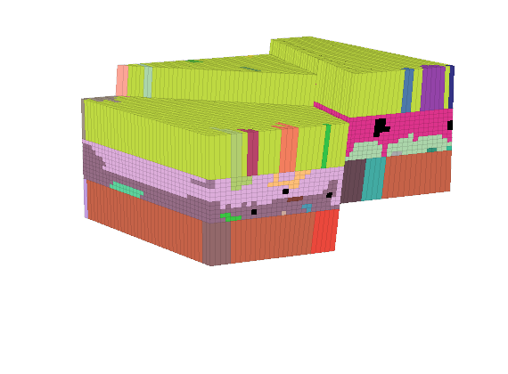
Remove confined blocks
%[cb,p] = findConfinedBlocks(G,p);
figure(1); clf,
hp = plotCellData(G, p,'EdgeAlpha',.1);
mp = max(p);
caxis([.5 mp+.5]); colormap(.8*tatarizeMap(mp)+.2*ones(mp,3));
view(-120,15), axis tight off, set(gca,'Projection','Perspective');
[hc,hh] = colorbarHist(p, [.5 mp+.5], 'South', mp);
bar(hh,log10(accumarray(p,1)),'FaceColor','none');
set(hh,'XLim',[.5 mp+.5]);
axis(hh,'off');
set(hc,'FontSize',14);

Remove recursively confined blocks
The implementation in findConfinedBlocks is relatively simple and does not work properly for recursivley confined blocks. For this, we can instead use graph algorithms from the MATLAB Boost Graph Library.
mrstModule add matlab_bgl
figure('Position',[450 540 940 260]);
G = computeGeometry(cartGrid([7 7]));
% p = ones(7,7); p(2:6,2:6)=2; p(3:5,3:5)=3;p(4,4)=4;
p = ones(7,7);p(:,4:7)=2;p(2:6,2:6)=3;p(3:5,3)=4;p(3:5,4)=5;p(3:5,5)=6;
pn = removeConfinedBlocks(G,p(:));
[~,pm] = findConfinedBlocks(G, p(:));
subplot(1,3,1), plotCellData(G,p(:)); axis equal off, caxis([1 7]), title('initial');
subplot(1,3,2), plotCellData(G,pm); axis equal off, caxis([1 7]), title('findConfinedBlocks');
subplot(1,3,3), plotCellData(G,pn); axis equal off, caxis([1 7]), title('removeConfinedBlocks');
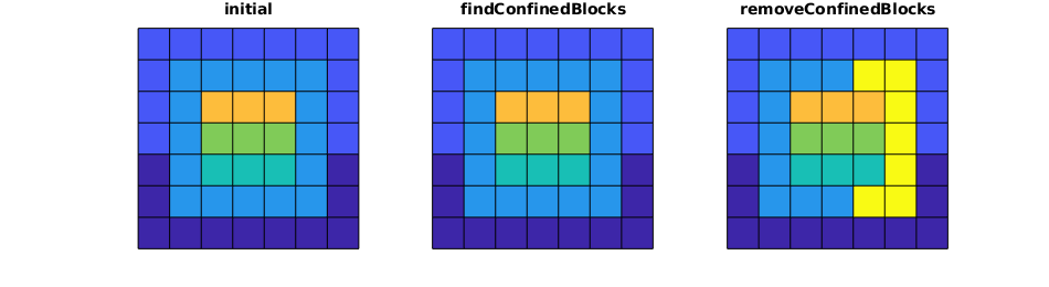
—— M E R G I N G F U N C T I O N S ——
G = computeGeometry(cartGrid([5 4]));
I = [1 1 5 2 2; 1 5 1 1 1; 4 5 1 2 2; 6 1 3 3 3]'; I=I(:);
p = segmentIndicator(G, I, 6);
n = G.cells.num;
set(figure(1),'Position',[450 540 940 260]);
subplot(1,3,1), cla
plotCellData(G,I,'edgecolor','none');
outlineCoarseGrid(G, p, 'k', 'LineWidth',2); axis off
colormap(.6*tatarizeMap(6)+.4*ones(6,3));
hold on
for i=1:n,
text(G.cells.centroids(i,1),G.cells.centroids(i,2), num2str(I(i)));
end
hold off
% mergeBlocks
p1 = mergeBlocks(p, G, ones(n,1), I, 2);
subplot(1,3,2), cla
plotCellData(G,I,'EdgeColor','none');
outlineCoarseGrid(G, p1, 'k', 'LineWidth', 2); axis off
xm = sparse(p1,1:n,1)*[G.cells.centroids, ones(n,1), I];
Ib = xm(:,end);
xm = bsxfun(@rdivide, xm(:,1:2), xm(:,3));
for i=1:size(xm,1)
text(xm(i,1),xm(i,2),num2str(Ib(i,end)));
end
% mergeBlocks2
p2 = mergeBlocks2(p, G, ones(G.cells.num,1), I, 2, 3);
subplot(1,3,3), cla
plotCellData(G,I,'EdgeColor','none');
outlineCoarseGrid(G, p2, 'k', 'LineWidth', 2); axis off
xm = sparse(p2,1:n,1)*[G.cells.centroids, ones(n,1), I];
Ib = xm(:,end);
xm = bsxfun(@rdivide, xm(:,1:2), xm(:,3));
for i=1:size(xm,1)
text(xm(i,1),xm(i,2),num2str(Ib(i,end)));
end
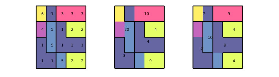
—— R E F I N E M E N T M E T H O D S —–
pargs={'EdgeColor','none'};
blk = [5 13];
dim = {[4,4],[5,5]};
for n=1:2
G = computeGeometry(cartGrid(dim{n}));
I = ones(G.cells.num,1);
figure('Position', [440 560 930 240]);
subplot(1,6,1);
plotGrid(G,'FaceColor','none'); axis equal off
for i=1:G.cells.num,
text(G.cells.centroids(i,1),G.cells.centroids(i,2),num2str(i),...
'HorizontalAlignment','center','FontSize',8);
end
p = refineUniform(I,G,I,4,'CartDims',[2,2]);
subplot(1,6,2); plotCellData(G,p,pargs{:}); axis equal off
outlineCoarseGrid(G,p,'k'); caxis([.5 blk(n)+.5]);
title('refineUniform','Position',[dim{n} 1].*[.5 1.02 1.02]);
p = refineGreedy(I,G,I,4,'nlevel',n);
subplot(1,6,3), plotCellData(G,p,pargs{:}); axis equal off,
outlineCoarseGrid(G,p,'k');caxis([.5 blk(n)+.5]);
title('refineGreedy','Position',[dim{n} 1].*[.5 1.02 1.02]);
p = refineGreedy2(I,G,I,4,'nlevel',n);
subplot(1,6,4), plotCellData(G,p,pargs{:}); axis equal off,
outlineCoarseGrid(G,p,'k'); caxis([.5 blk(n)+.5]);
title('refineGreedy2','Position',[dim{n} 1].*[.5 1.02 1.02]);
p = refineGreedy3(I,G,I,4,'nlevel',n);
subplot(1,6,5), plotCellData(G,p,pargs{:}); axis equal off,
outlineCoarseGrid(G,p,'k');caxis([.5 blk(n)+.5]);
title('refineGreedy3','Position',[dim{n} 1].*[.5 1.02 1.02]);
p = refineGreedy4(I,G,I,4,'nlevel',n);
subplot(1,6,6), plotCellData(G,p,pargs{:}); title('refineGreedy4');axis equal off,
outlineCoarseGrid(G,p,'k');caxis([.5 blk(n)+.5]);
title('refineGreedy4','Position',[dim{n} 1].*[.5 1.02 1.02]);
colormap(.8*tatarizeMap(blk(n))+.2*ones(blk(n),3));
h = colorbar('horiz');
set(h,'Position',[0.29 0.13 0.455 0.1],'XTick',1:blk(n));
end
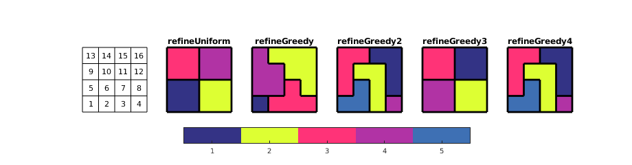
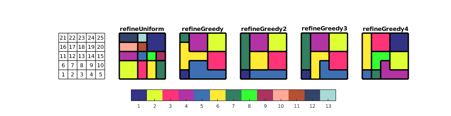
Simple Model of an Anticline
Generated from showAnticlineModel.m
Conceptual illustration of a reservoir model with aggressive coarsening in the aquifer zone, modest coarsening above the initial water contact, and original resolution for cells with low residence time
mrstModule add coarsegrid diagnostics incomp spe10
Cartesian grid and rock parameters
[nx,ny,nz] = deal(60,60,15);
G = cartGrid([nx ny nz], [nx ny nz].*[20 10 2]*ft);
rock = getSPE10rock(1:nx,1:ny,nz:-1:1);
rock.poro(rock.poro==0) = 1e-5;
Make anticline structure
x = G.nodes.coords(:,1);
y = G.nodes.coords(:,2);
normalize = @(x) (x-min(x))/(max(x)-min(x));
x = 2*normalize(x)-1;
y = 2*normalize(y)-1;
r = min(sqrt(x.^2 + y.^2),1);
dz = r.^2 ./ (r.^2 + (1-r).^4);
G.nodes.coords(:,3) = G.nodes.coords(:,3) + dz*(nz+1)*2*ft;
G = computeGeometry(G);
clf, set(gcf,'Position', [230 190 1200 630]);
subplot(1,3,1)
plotCellData(G,log10(rock.perm(:,1)),'EdgeColor','none');
view(-54,30); set(gca,'dataasp',[1 1 .4]), axis tight off
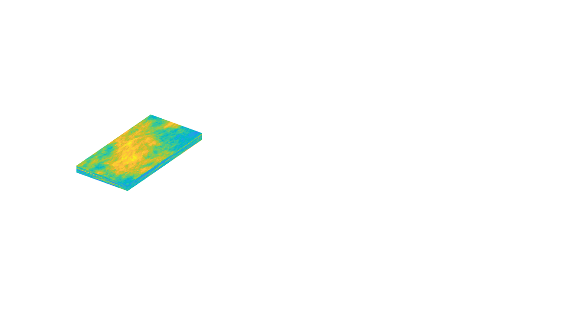
Set initial saturation
s = zeros(G.cells.num,1);
s(G.cells.centroids(:,3)>(nz+1)*2*ft) = 1;
%[nodes,pos] = gridCellNodes(G, (1:G.cells.num).');
%c = rldecode(1:G.cells.num, diff(pos), 2).';
%A = sparse(c,nodes,1)*[s, ones([G.nodes.num,1])];
%s = bsxfun(@rdivide, A(:,1:(end-1)), A(:,end));
subplot(1,3,2), cla
plotCellData(G,1-s,'EdgeAlpha',.1); caxis([0 1]);
view(-54,30); set(gca,'dataasp',[1 1 .4]), axis tight off

Set wells
producers
args = {'Type', 'bhp', 'Val', 100*barsa, 'Comp_i', [0 1], 'sign', -1};
W = verticalWell([], G, rock, 28, 30, [], args{:}, 'name', 'P1');
W = verticalWell(W, G, rock, 34, 32, [], args{:}, 'name', 'P2');
% injectors
args = {'Type', 'bhp', 'Val', 150*barsa, 'Comp_i', [1 0], 'sign', 1};
W = verticalWell(W, G, rock, 18, 18, [], args{:}, 'name', 'I1');
W = verticalWell(W, G, rock, 18, 44, [], args{:}, 'name', 'I2');
W = verticalWell(W, G, rock, 44, 44, [], args{:}, 'name', 'I4');
subplot(1,3,1)
plotWell(G,W,'Color','k','FontSize',12); axis tight off
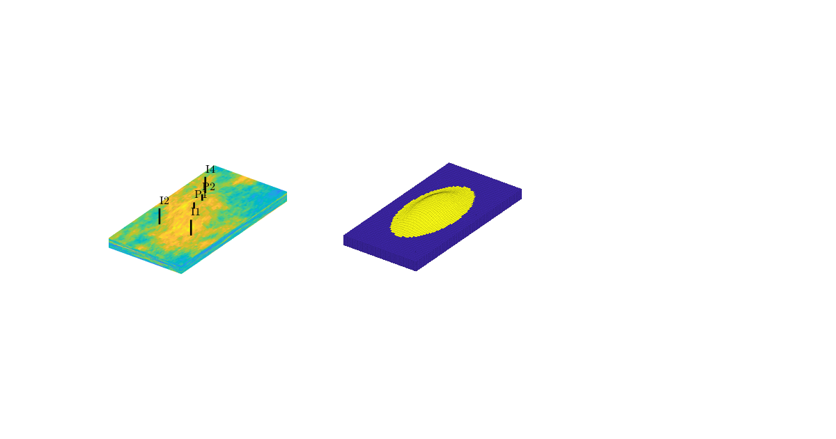
Incompressible pressure solution and time-of-flight
hT = computeTrans(G, rock);
fluid = initSimpleFluid('mu' , [1 1]*centi*poise , ...
'rho', [1014, 859]*kilogram/meter^3, ...
'n' , [ 2, 2]);
state = initState(G, W, 100*barsa, [s 1-s]);
state = incompTPFA(state, G, hT, fluid, 'wells', W);
Tf = computeTimeOfFlight(state, G, rock, 'wells', W, 'reverse', false);
Tb = computeTimeOfFlight(state, G, rock, 'wells', W, 'reverse', true);
T = Tf + Tb;
Extract the high-flow zones
Selection criterion: travel time less than two years (times magic factor)
tfac = median(T(vertcat(W.cells)));
I = T < 2*tfac;
subplot(1,3,3), cla
plotCellData(G,I+0,'EdgeAlpha',.1); caxis([-3 2]);
plotWell(G,W,'Color','w','FontSize',12);
view(-54,30); set(gca,'dataasp',[1 1 .4]), axis tight off
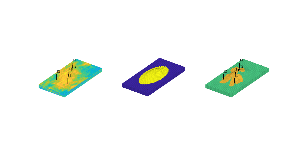
Coarsen model differently in aquifer, oil, and high-flow zones
Aquifer zone
pc = partitionCartGrid([nx,ny,nz],[10 10 5]);
p = compressPartition(pc);
% Zone above intial water contact
pf = partitionCartGrid([nx,ny,nz],[nx,ny,nz]/2);
p(s<1e-5) = pf(s<1e-5);
% Zone with low residence time
po = 1:G.cells.num;
p(I) = po(I);
% Near-well region
q = zeros(G.cells.num,1);
q(vertcat(W.cells))=1;
qc = accumarray(pc,q);
ind = qc(pc)>0;
p(ind) = po(ind);
subplot(1,3,1)
h = outlineCoarseGrid(G, p,'FaceColor','none','EdgeColor','k');
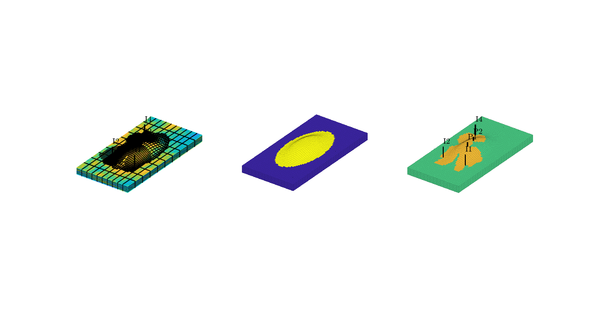
for i=1:3
subplot(1,3,i),
set(gca,'Clipping', 'off', ...
'Position',get(gca,'Position')+[-.025 -.025 .05 .05]); zoom(1.3*1.1);
end
colormap(.8*jet(128)+.2*ones(128,3));
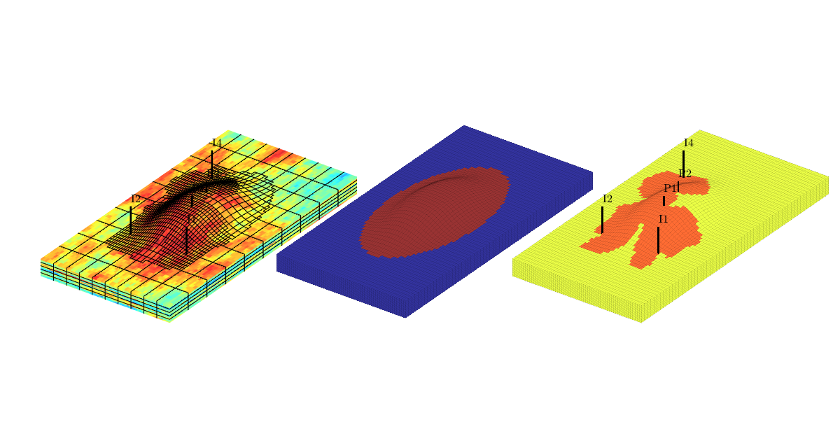
Stair-stepped grid
Generated from showCaseB.m
clf
grdecl = readGRDECL(fullfile(getDatasetPath('CaseB4'),'stairstep_36x48.grdecl'));
Gs = processGRDECL(grdecl);
Gs = computeGeometry(Gs);
Kx = logNormLayers(Gs.cartDims, [10 50 400 50 10], ...
'indices', [1 2 5 8 12 13]); Kx = log10(Kx);
plotCellData(Gs,Kx(Gs.cells.indexMap),'EdgeColor','k');
set(gca,'dataa',[15 20 1])
axis tight off, view(150,30), zoom(1.2)
set(gca,'Clipping','off')
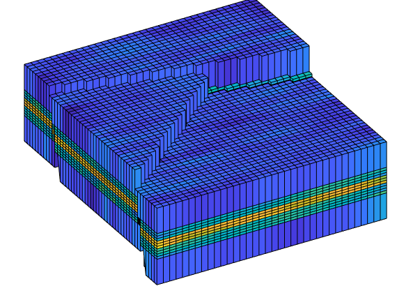
cut_grdecl = cutGrdecl(grdecl, [12 20; 13 23; 1 12]);
k = reshape(Kx,Gs.cartDims);
kx = reshape(k(12:20,13:23,1:12),1,[]);
g = processGRDECL(cut_grdecl);
clf
plotCellData(g,kx(g.cells.indexMap)','EdgeColor','k'),
axis tight off, view(150,50), zoom(1.2)
set(gca,'Clipping','off')
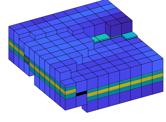
Corner-point grid
clf
grdecl = readGRDECL(fullfile(getDatasetPath('CaseB4'),'pillar_36x48.grdecl'));
Gp = processGRDECL(grdecl);
Gp = computeGeometry(Gp);
plotCellData(Gp,Kx(Gp.cells.indexMap),'EdgeColor','k');
set(gca,'dataa',[15 20 1])
axis tight off, view(150,30), zoom(1.2)
set(gca,'Clipping','off')
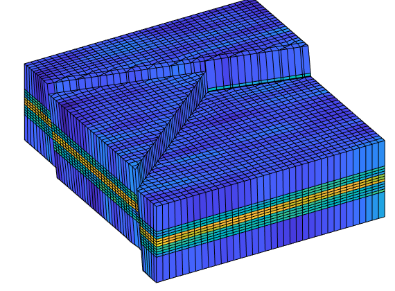
cut_grdecl = cutGrdecl(grdecl, [12 20; 13 23; 1 12]);
g = processGRDECL(cut_grdecl);
clf
plotCellData(g,kx(g.cells.indexMap)','EdgeColor','k'),
axis tight off, view(150,50), zoom(1.2)
set(gca,'Clipping','off')
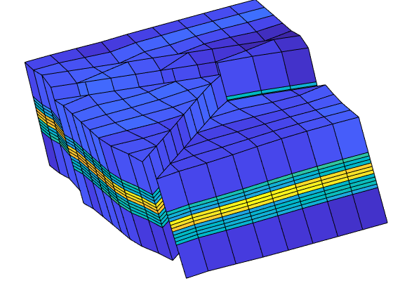
Visualize results
lf
set(gcf,'Position', [300 450 1000 330]);
subplot(1,2,1);
plotCellData(Gs, log10(Kx(Gs.cells.indexMap)), 'EdgeColor', 'k', 'EdgeAlpha',0.1);
set(gca,'dataaspect',[32 44 2.5])
axis tight off, view(104,28);
%
subplot(1,2,2);
plotCellData(Gp, log10(Kx(Gp.cells.indexMap)),'EdgeColor', 'k', 'EdgeAlpha',0.1);
set(gca,'dataaspect',[32 44 2.5])
axis tight off, view(104,28);
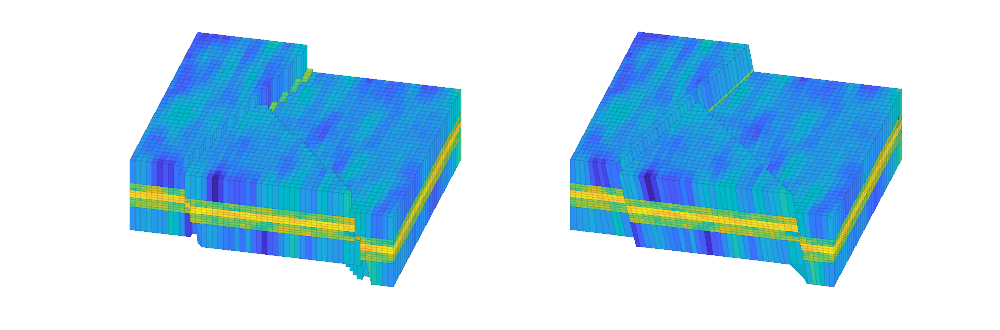
Examples of How to Generate Coarse Grids
Generated from showCoarseGrid.m
We show three examples: a 2x2 partition of a 4x4 Cartesian grid, a 2x2 partition of a facies model with subpartition of coarse faces, and a 3D model with subdivision of coarse faces
mrstModule add coarsegrid;
First example: 2x2 partition of a 4x4 Cartesian grid
G = computeGeometry(cartGrid([4,4]));
p = partitionUI(G, [2,2]);
CG = generateCoarseGrid(G, p);
clf
plotCellData(G,(1:G.cells.num)','LineStyle',':');
plotGrid(CG,'faceColor','none','LineWidth',3);
colormap((jet(G.cells.num)+repmat(2,G.cells.num,3))/3);
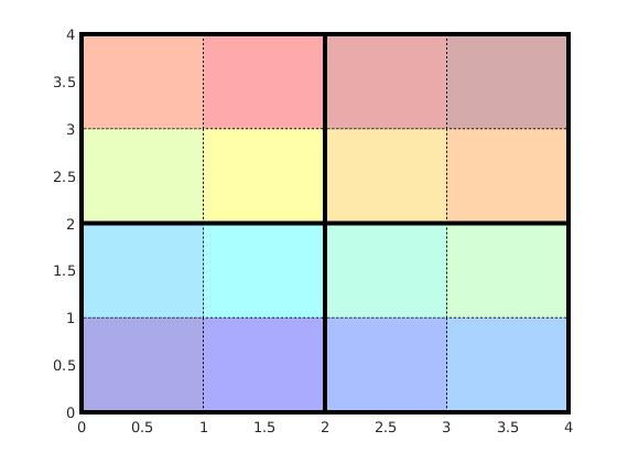
Show cell/block indices
CG = coarsenGeometry(CG);
tg = text(G.cells.centroids(:,1), G.cells.centroids(:,2), ...
num2str((1:G.cells.num)'),'FontSize',20, 'HorizontalAlignment','center');
tcg = text(CG.cells.centroids(:,1), CG.cells.centroids(:,2), ...
num2str((1:CG.cells.num)'),'FontSize',24, 'HorizontalAlignment','center');
axis off;
set(tcg,'BackgroundColor','w','EdgeColor','none');
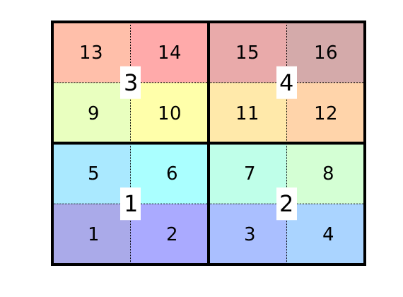
Show indices of the faces in the fine/coarse grids
delete([tg; tcg]);
tg = text(G.faces.centroids(:,1), G.faces.centroids(:,2), ...
num2str((1:G.faces.num)'),'FontSize',18, 'HorizontalAlignment','center');
tcg = text(CG.faces.centroids(:,1), CG.faces.centroids(:,2), ...
num2str((1:CG.faces.num)'),'FontSize',24, 'HorizontalAlignment','center');
set(tcg,'BackgroundColor','w','EdgeColor','k');
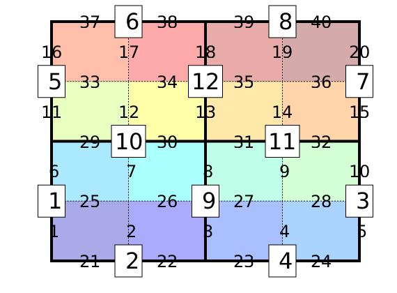
Second example: 2D face partition
clf;
G = computeGeometry(cartGrid([8, 8], [1 1]));
f = @(c) sin(3*pi*(c(:,1)-c(:,2)));
pf = 1 + (f(G.cells.centroids) > 0);
plotCellData(G, pf,'edgecolor','none'); axis off;
colormap(.2*gray(2)+.8*ones(2,3));
pv = partitionCartGrid(G.cartDims, [2 2]);
pf = cellPartitionToFacePartition(G,pf);
pf = processFacePartition(G, pv, pf);
CG = generateCoarseGrid(G, pv, pf);
CG = coarsenGeometry(CG);
cmap = lines(CG.faces.num);
for i=1:CG.faces.num
plotFaces(CG,i,'LineWidth',6,'EdgeColor', cmap(i,:));
end
text(CG.faces.centroids(:,1), CG.faces.centroids(:,2), ...
num2str((1:CG.faces.num)'),'FontSize',20,'HorizontalAlignment','center');
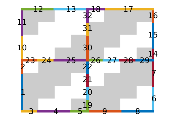
Third example: 3D face partition
clf
G = computeGeometry(cartGrid([20 20 6]));
c = G.cells.centroids;
G = removeCells(G, ...
(c(:,1)<10) & (c(:,2)<10) & (c(:,3)<3));
plotGrid(G,'FaceColor',[1 1 .7]); view(3); axis off
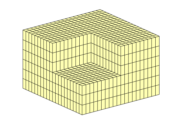
clf
p = partitionUI(G,[2, 2, 2]);
q = partitionUI(G,[4, 4, 2]);
CG = generateCoarseGrid(G, p, ...
cellPartitionToFacePartition(G,q));
plotCellData(CG,(1:max(p))');
plotFaces(CG,1:CG.faces.num,...
'FaceColor' , 'none' , 'LineWidth' ,2);
view(3); axis off
colormap(.5*(jet(128)+ones(128,3)));

Add face centroids
CG = coarsenGeometry(CG);
plotCentroids = @(pts, varargin) ...
plot3(pts(:,1), pts(:,2), pts(:,3), varargin{:});
hold on
h=plotCentroids(CG.faces.centroids, 'k*');
hold off;
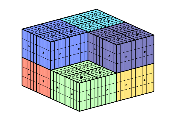
The coarse grid also contains lookup tables for mapping blocks and interfaces in the coarse grid to cells and faces in the fine grid. To demonstrate this, we visualize a single coarse face consisting of several fine faces along with the cells its block neighbors in red and blue respectively on the fine grid.
ace = 66;
sub = CG.faces.connPos(face):CG.faces.connPos(face+1)-1;
ff = CG.faces.fconn(sub);
neigh = CG.faces.neighbors(face,:);
clf
show = false(1,CG.faces.num);
show(boundaryFaces(CG)) = true;
show(boundaryFaces(CG,neigh)) = false;
plotFaces(CG, show,'FaceColor',[1 1 .7]);
plotFaces(CG,boundaryFaces(CG,neigh),'FaceColor','none','LineWidth', 2);
plotFaces(G, ff, 'FaceColor', 'g')
plotGrid(G, p == neigh(1), 'FaceColor', 'none', 'EdgeColor', 'r')
plotGrid(G, p == neigh(2), 'FaceColor', 'none', 'EdgeColor', 'b')
view(3); axis off
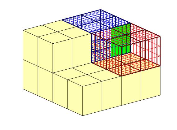
Illustration of Geometry Computation for a Hexahedral Cell
Generated from showComputeGeometry.m
We go through the computation of geometry information, step by step, for a hexahedral cell with skewed geometry
Construct model
G = cartGrid([1 1 1]);
G.nodes.coords(1:end/2,:) = G.nodes.coords(1:end/2,:)*0.75;
G = computeGeometry(G);
Add face number, etc
clf
plotGrid(G,'FaceColor',[.7 .7 .7], 'FaceAlpha',.7);
hold on
plot3(G.faces.centroids(:,1),G.faces.centroids(:,2),G.faces.centroids(:,3),...
'sr','MarkerSize', 24, 'LineWidth',1.5);
text(G.faces.centroids(:,1),G.faces.centroids(:,2),G.faces.centroids(:,3),...
num2str((1:G.faces.num)'),'HorizontalAlignment','center',...
'Color','r', 'FontWeight','demi','FontSize', 20);
plot3(G.nodes.coords(:,1),G.nodes.coords(:,2),G.nodes.coords(:,3),...
'ob','MarkerSize', 24, 'LineWidth',1.5);
text(G.nodes.coords(:,1),G.nodes.coords(:,2),G.nodes.coords(:,3),...
num2str((1:G.nodes.num)'),'HorizontalAlignment','center',...
'Color','b', 'FontWeight','demi','FontSize', 20);
hold off
view(50,25), axis tight off
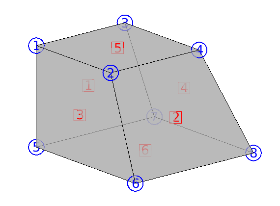
Computation of face areas, normals, and centroids
faceNo = rldecode(1:G.faces.num, diff(G.faces.nodePos), 2) .';
nodes=[(1:numel(G.faces.nodes))' faceNo G.faces.nodes]; disp(nodes)
p = G.faces.nodePos;
n = (2:size(G.faces.nodes, 1)+1) .';
n(p(2 : end) - 1) = p(1 : end-1);
localEdge2Face = sparse(1 : numel(G.faces.nodes), faceNo, 1, ...
numel(G.faces.nodes), G.faces.num);
pC = bsxfun(@rdivide, localEdge2Face.' * G.nodes.coords(G.faces.nodes,:), ...
diff(double(G.faces.nodePos)));
pC = localEdge2Face * pC;
pt1 = G.nodes.coords(G.faces.nodes,:);
pt2 = G.nodes.coords(G.faces.nodes(n),:);
v1 = pt2 - pt1;
v2 = pC - pt1;
sN = cross(v1,v2)./2;
sC = (pt1 + pt2 + pC)/3;
sA = sqrt(sum(sN.^2, 2));
N = localEdge2Face.' * sN;
A = localEdge2Face.' * sA;
C = bsxfun(@rdivide, localEdge2Face.'* bsxfun(@times, sA, sC), A);
sNs = sign(sum(sN.*(localEdge2Face*N),2));
1 1 1
2 1 3
3 1 7
4 1 5
5 2 2
6 2 4
7 2 8
8 2 6
...
clf,
T = [pt1 pt2 pC]; T = T(:,[1 4 7 2 5 8 3 6 9]);
patch(T(:,1:3)',T(:,4:6)',T(:,7:9)',[.7 .7 .7],'FaceAlpha',0.9);
i = 5:8;
hold on
quiver3(pt1(i,1),pt1(i,2),pt1(i,3),v1(i,1),v1(i,2),v1(i,3),'LineWidth',2);
quiver3(pt1(i,1),pt1(i,2),pt1(i,3),v2(i,1),v2(i,2),v2(i,3),'LineWidth',2);
quiver3(pt1(i,1),pt1(i,2),pt1(i,3),sN(i,1),sN(i,2),sN(i,3),'LineWidth',2);
plot3(sC(i,1)+.01,sC(i,2),sC(i,3),'or');
hold off;
view(50,25), axis tight off, zoom(1.2), set(gca,'zdir','reverse');
set(gca,'Clipping','off')
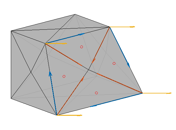
cla,
patch(T(:,1:3)',T(:,4:6)',T(:,7:9)',[.7 .7 .7],'FaceAlpha',0.9);
hold on
plot3(C(:,1),C(:,2),C(:,3),'.k','MarkerSize',20)
quiver3(C(2,1),C(2,2),C(2,3),N(2,1),N(2,2),N(2,3),'LineWidth',2);
hold off
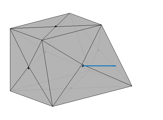
Computing cell volumes and centroids
nF = G.cells.facePos(2)-G.cells.facePos(1);
inx = 1:nF;
faces = G.cells.faces(inx,1);
[triE, triF] = find(localEdge2Face(:,faces));
fC = C(faces,:);
cC = sum(fC)./double(nF);
relSubC = bsxfun(@minus, sC(triE,:),cC);
orient = 2*double(G.faces.neighbors(G.cells.faces(inx,1), 1) == 1) - 1;
oN = bsxfun(@times, sN(triE,:), sNs(triE).*orient(triF) );
lf
X = [G.nodes.coords; pC(G.faces.nodePos(1:end-1),:); cC];
T = [G.faces.nodes, G.faces.nodes(n), faceNo+G.nodes.num, ...
repmat(G.nodes.num+G.faces.num+1,numel(faceNo),1)];
h=tetramesh(T,X); set(h,'FaceColor',[.7 .7 .7],'facealpha',.15);
hold on;
i = [5:12 17:20];
h=tetramesh(T([3 7 10 14],:),X); set(h,'FaceColor','y','facealpha',.9);
quiver3(sC(i,1),sC(i,2),sC(i,3),oN(i,1),oN(i,2),oN(i,3),'LineWidth',2);
quiver3(sC(i,1),sC(i,2),sC(i,3),...
relSubC(i,1),relSubC(i,2),relSubC(i,3),'LineWidth',2);
hold off;
view(75,30), axis tight off, zoom(1.3), set(gca,'zdir','reverse');
set(gca,'Clipping','off')
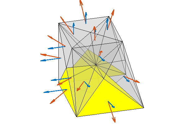
Show Geometry Computation for a PEBI Cell
Generated from showComputeGeometryPEBI.m
We go through the computation of geometry information, step by step, for a polyhedral cell from a 2.5D PEBI model used in industry. The cell is not exactly the same one as shown in the book.
load data/pebi-cell.mat;
Add face number, etc
clf
plotGrid(G,'FaceColor',[.7 .7 .7], 'FaceAlpha',.7); set(gca,'zdir','normal');
hold on
plot3(G.faces.centroids(:,1),G.faces.centroids(:,2),G.faces.centroids(:,3),...
'sr','MarkerSize', 30, 'LineWidth',1.5);
text(G.faces.centroids(:,1),G.faces.centroids(:,2),G.faces.centroids(:,3),...
num2str((1:G.faces.num)'),'HorizontalAlignment','center',...
'Color','r', 'FontWeight','demi','FontSize',24);
plot3(G.nodes.coords(:,1),G.nodes.coords(:,2),G.nodes.coords(:,3),...
'ob','MarkerSize', 30, 'LineWidth',1.5);
text(G.nodes.coords(:,1),G.nodes.coords(:,2),G.nodes.coords(:,3),...
num2str((1:G.nodes.num)'),'HorizontalAlignment','center',...
'Color','b', 'FontWeight','demi','FontSize',24);
hold off
view(20,15), axis tight off, zoom(1.2)
set(gca,'Clipping','off')
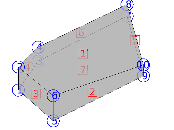
Computation of face areas, normals, and centroids
faceNo = rldecode(1:G.faces.num, diff(G.faces.nodePos), 2) .';
nodes=[(1:numel(G.faces.nodes))' faceNo G.faces.nodes]; disp(nodes)
p = G.faces.nodePos;
n = (2:size(G.faces.nodes, 1)+1) .';
n(p(2 : end) - 1) = p(1 : end-1);
localEdge2Face = sparse(1 : numel(G.faces.nodes), faceNo, 1, ...
numel(G.faces.nodes), G.faces.num);
pC = bsxfun(@rdivide, localEdge2Face.' * G.nodes.coords(G.faces.nodes,:), ...
diff(double(G.faces.nodePos)));
pC = localEdge2Face * pC;
pt1 = G.nodes.coords(G.faces.nodes,:);
pt2 = G.nodes.coords(G.faces.nodes(n),:);
v1 = pt2 - pt1;
v2 = pC - pt1;
sN = cross(v1,v2)./2;
sC = (pt1 + pt2 + pC)/3;
sA = sqrt(sum(sN.^2, 2));
N = localEdge2Face.' * sN;
A = localEdge2Face.' * sA;
C = bsxfun(@rdivide, localEdge2Face.'* bsxfun(@times, sA, sC), A);
sNs = sign(sum(sN.*(localEdge2Face*N),2));
1 1 6
2 1 10
3 1 8
4 1 4
5 1 2
6 2 9
7 2 10
8 2 6
...
clf,
T = [pt1 pt2 pC]; T = T(:,[1 4 7 2 5 8 3 6 9]);
patch(T(:,1:3)',T(:,4:6)',T(:,7:9)',[.7 .7 .7],'FaceAlpha',0.9);
i = 1:5;
hold on
quiver3(pt1(i,1),pt1(i,2),pt1(i,3),v1(i,1),v1(i,2),v1(i,3),'LineWidth',2);
quiver3(pt1(i,1),pt1(i,2),pt1(i,3),v2(i,1),v2(i,2),v2(i,3),'LineWidth',2);
quiver3(pt1(i,1),pt1(i,2),pt1(i,3),sN(i,1),sN(i,2),sN(i,3),.003,'LineWidth',2);
plot3(sC(i,1)+.01,sC(i,2),sC(i,3),'or');
hold off;
view(20,15), axis tight off, zoom(1.3)
set(gca,'Clipping','off')
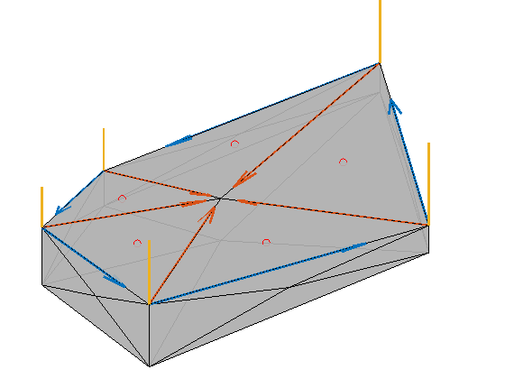
cla,
patch(T(:,1:3)',T(:,4:6)',T(:,7:9)',[.7 .7 .7],'FaceAlpha',0.9);
hold on
plot3(C(:,1),C(:,2),C(:,3),'.k','MarkerSize',20)
quiver3(C(1,1),C(1,2),C(1,3),N(1,1)/2e5,N(1,2)/2e5,N(1,3)/2e5,'LineWidth',2);
hold off
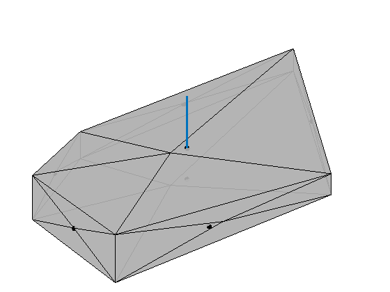
Computing cell volumes and centroids
nF = G.cells.facePos(2)-G.cells.facePos(1);
inx = 1:nF;
faces = G.cells.faces(inx,1);
[triE, triF] = find(localEdge2Face(:,faces));
fC = C(faces,:);
cC = sum(fC)./double(nF);
relSubC = bsxfun(@minus, sC(triE,:),cC);
orient = 2*double(G.faces.neighbors(G.cells.faces(inx,1), 1) == 1) - 1;
oN = bsxfun(@times, sN(triE,:), sNs(triE).*orient(triF) );
lf
X = [G.nodes.coords; pC(G.faces.nodePos(1:end-1),:); cC];
T = [G.faces.nodes, G.faces.nodes(n), faceNo+G.nodes.num, ...
repmat(G.nodes.num+G.faces.num+1,numel(faceNo),1)];
h=tetramesh(T,X); set(h,'FaceColor',[.7 .7 .7],'facealpha',.15);
set(gca,'dataasp',[1 1 8e-3])
view(20,15), axis tight off, zoom(1.3), %set(gca,'zdir','reverse');
set(gca,'Clipping','off')
hold on;
ix = [2 18 19 20 21 27]
col = 'ywmrcgb';
for i=1:numel(ix)
h=tetramesh(T(ix(i),:),X); set(h,'FaceColor',col(mod(i,7)+1),'FaceAlpha',1);
end
ix = [5 13 12 11 10 30]
for i=1:numel(ix)
h=tetramesh(T(ix(i),:),X); set(h,'FaceColor',col(mod(i,7)+1),'FaceAlpha',1);
end
i=1:5;
h=quiver3(sC(i,1),sC(i,2),sC(i,3),oN(i,1),oN(i,2),oN(i,3),2e-2,'LineWidth',2);
quiver3(sC(i,1),sC(i,2),sC(i,3),...
relSubC(i,1),relSubC(i,2),relSubC(i,3),.5,'LineWidth',2);
hold off
ix =
2 18 19 20 21 27
ix =
...
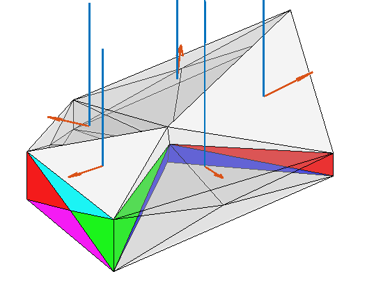
Example of Realistic Corner-Point Geometry: SAIGUP
Generated from showGridSAIGUP.m
The <http://www.fault-analysis-group.ucd.ie/Projects/SAIGUP.html>SAIGUP project is a systematic assessment of uncertainty in reserves and production estimates within an objectively defined geological parameterisation encompassing the majority of European clastic oil reservoirs. A broad suite of shallow marine sedimentological reservoir types are indexed to continuously varying 3D anisotropy and heterogeneity levels. Structural complexity ranges from unfaulted to compartmentalised, and fault types from transmissive to sealing. Several geostatistical realisations each for the geologically diverse reservoir types covering the pre-defined parameter-space are up-scaled, faulted and simulated with an appropriate production strategy for an approximately 20 year period. Herein, we will inspect in detail one instance of the model, which can be downloaded from the <http://www.sintef.no/Projectweb/MRST>MRST webpage
Load data and convert units
We start by reading the model from a file in the Eclipse format (GRDECL) that can be read using the readGRDECL function. (If the model is not available the getDatasetPath function will download and install it for you).
grdecl = fullfile(getDatasetPath('SAIGUP'), 'SAIGUP.GRDECL');
grdecl = readGRDECL(grdecl);
usys = getUnitSystem('METRIC');
grdecl = convertInputUnits(grdecl, usys);
Inspect full model
G = processGRDECL(grdecl, 'Verbose', true);
Adding 9600 artificial cells at top/bottom
Processing regular i-faces
Found 79498 new regular faces
Elapsed time is 0.027229 seconds.
Processing i-faces on faults
Found 521 faulted stacks
...
G = computeGeometry(G);
rock = grdecl2Rock(grdecl, G.cells.indexMap);
Inspect geometry
Construct pillars and corner-points to verify the resolution of the model
[X,Y,Z] = buildCornerPtPillars(grdecl,'Scale',true); %#ok<NASGU>
dx = unique(diff(X)).' %#ok<NOPTS>
[x,y,z] = buildCornerPtNodes(grdecl); %#ok<ASGLU>
dz = unique(reshape(diff(z,1,3),1,[])) %#ok<NOPTS>
clear x y z X Y Z
dx =
-3000 75
dz =
...
Next, we look at small faces created to enforce a matching grid. Vertical faces that are not subdividided will be parallelograms with a 300 m^2 area. We therefore look at faces having smaller area
hist(G.faces.areas(G.faces.areas<300),100);
xlabel('Face area, m^2');
disp(['Area less than 0.01 m^2: ', num2str(sum(G.faces.areas<0.01))])
disp(['Area less than 0.10 m^2: ', num2str(sum(G.faces.areas<0.1))])
disp(['Area less than 1.00 m^2: ', num2str(sum(G.faces.areas<1))])
Area less than 0.01 m^2: 43
Area less than 0.10 m^2: 202
Area less than 1.00 m^2: 868
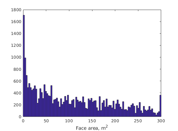
Plot where these faces appear in the model
clf
plotGrid(G,'FaceColor','none','EdgeAlpha',0.1);
plotFaces(G,find(G.faces.tag>0 & G.faces.areas>=290),'y','edgea',0.1);
plotFaces(G,find(G.faces.areas<290),'r','edgea',0.1);
view(-105,45), axis tight off
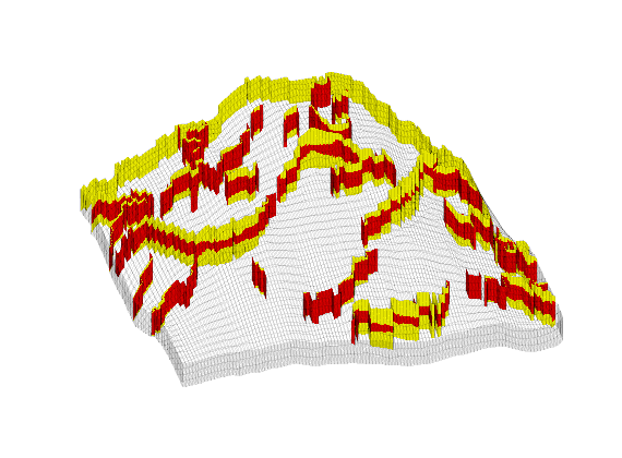
Process the model using a tolerance to get rid of the smallest faces
for a=[0.05 0.1 .25 0.5 1]
G2 = processGRDECL(grdecl, 'Tolerance', a);
G2 = computeGeometry(G2);
disp([ a, min(G2.faces.areas)])
end
clear G2
0.0500 0.0318
0.1000 0.0268
0.2500 0.0966
0.5000 0.6048
...
The layered structure
Show layered structure using a very simple trick: create a matrix with ones in all cells of the logical Cartesian grid and then do a cummulative summation in the vertical direction to get increasing values.
clf, args = {'EdgeColor','k','EdgeAlpha',0.1};
val = cumsum(ones(G.cartDims),3);
plotCellData(G,val(G.cells.indexMap),args{:});
view(-80,50), axis off tight
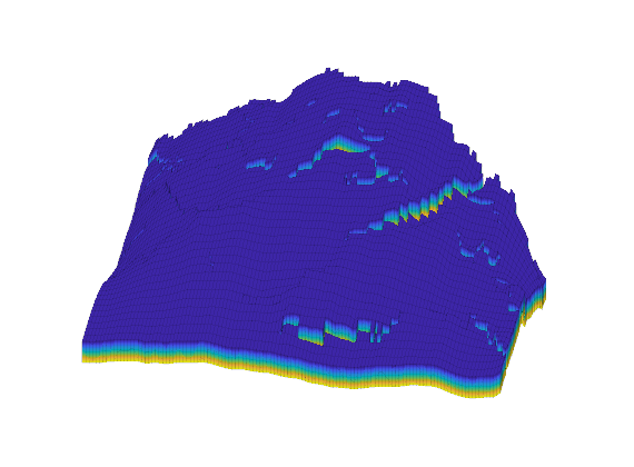
Unfortunately, our attempt at visualizing the layered structure was not very successful. We therefore try to extract and visualize only the cells that are adjacent to a fault.
cellList = G.faces.neighbors(G.faces.tag>0, :);
cells = unique(cellList(cellList>0));
cla,
plotCellData(G,val(G.cells.indexMap),cells,args{:});
view(-120,40)
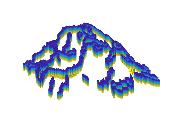
Restrict the plot to only parts of the grid using ismember, which uses O(n log n) operations
clear ijk
[ijk{1:3}] = ind2sub(G.cartDims, G.cells.indexMap); ijk = [ijk{:}];
[I,J,K] = meshgrid(1:9,1:30,1:20);
bndBox = find(ismember(ijk,[I(:), J(:), K(:)],'rows'));
inspect = cells(ismember(cells,bndBox));
cla,
plotCellData(G,val(G.cells.indexMap), inspect,'EdgeColor','k');
axis tight off

Restrict the plot to only parts of the grid using logical indexing which uses O(n) operations
clear ijk
[ijk{1:3}] = ind2sub(G.cartDims, G.cells.indexMap);
I = false(G.cartDims(1),1); I(1:9)=true;
J = false(G.cartDims(2),1); J(1:30)=true;
K = false(G.cartDims(3),1); K(1:20)=true;
pick = I(ijk{1}) & J(ijk{2}) & K(ijk{3});
pick2 = false(G.cells.num,1); pick2(cells) = true;
inspect = find(pick & pick2);
cla,
plotCellData(G,val(G.cells.indexMap), inspect,'EdgeColor','k');
axis tight off
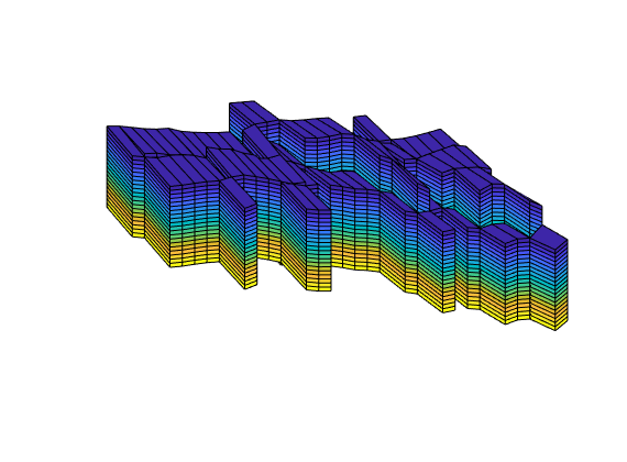
Let us now try to also colour the faces of the model
cellno = gridCellNo(G);
faces = unique(G.cells.faces(pick(cellno), 1));
inspect = faces(G.faces.tag(faces)>0);
plotFaces(G,inspect,[.7 .7 .7],'edgec','r');
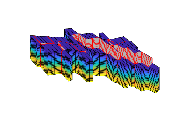
Making a ribbon plot
lear ijk;
[ijk{1:3}] = ind2sub(G.cartDims, G.cells.indexMap);
% Ribbon in x-direction
I = false(G.cartDims(1),1); I(1:5:end)=true;
J = true(G.cartDims(2),1);
K = true(G.cartDims(3),1);
pickX = I(ijk{1}) & J(ijk{2}) & K(ijk{3});
% Ribbon in y-direction
I = true(G.cartDims(1),1);
J = false(G.cartDims(2),1); J(1:10:end) = true;
K = true(G.cartDims(3),1);
pickY = I(ijk{1}) & J(ijk{2}) & K(ijk{3});
clf,
plotCellData(G,rock.poro, pickX | pickY,'EdgeColor','k','EdgeAlpha',0.1);
view(-100,45), axis tight off
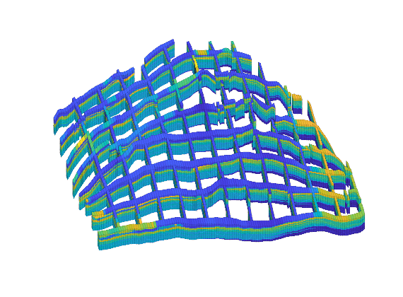
Graphical View of the Grid Structure
Generated from showGridStructure.m
In this example, we will show details of the grid structures for three different grids: a Cartesian grid with one cell removed, a triangular grid, and a Voronoi grid. The examples will show cell numbers, node numbers, and face numbers.
REGULAR GRID
G = removeCells( cartGrid([3,2]), 2);
G = computeGeometry(G);
Plot cell, face, and node numbers
newplot;
plotGrid(G,'FaceColor',[0.95 0.95 0.95]); axis off;
hold on;
text(G.cells.centroids(:,1)-0.04, ...
G.cells.centroids(:,2), num2str((1:G.cells.num)'),'FontSize',20);
plot(G.cells.centroids(:,1),...
G.cells.centroids(:,2),'ok','MarkerSize',24);
text(G.faces.centroids(:,1)-0.045, G.faces.centroids(:,2), ...
num2str((1:G.faces.num)'),'FontSize',16);
text(G.nodes.coords(:,1)-0.075, ...
G.nodes.coords(:,2), num2str((1:G.nodes.num)'),'FontSize',18);
plot(G.nodes.coords(:,1),...
G.nodes.coords(:,2),'sk','MarkerSize',24);
hold off;
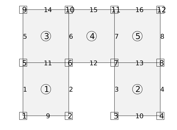
Output content of cells.faces, faces.nodes, and faces.neighbors to file
faces =[ rldecode(1 : G.cells.num,diff(G.cells.facePos), 2).' G.cells.faces];
tag = {'East'; 'West'; 'South'; 'North'; 'Bottom'; 'Top'};
fp = fopen('G-structured.txt','w');
fprintf(fp,'cells.faces =\n');
for i=1:size(faces,1)
fprintf(fp,' %3d %3d %3d [%s]\n', faces(i,1:3), tag{faces(i,3)});
end
nodes = [ rldecode(1:G.faces.num,diff(G.faces.nodePos), 2).' G.faces.nodes];
fprintf(fp,'\n\nfaces.nodes =\n');
fprintf(fp,' %3d %3d\n', nodes');
fprintf(fp,'\n\nfaces.neighbors =\n');
fprintf(fp,' %3d %3d\n', G.faces.neighbors');
fclose(fp);
UNSTRUCTURED TRIANGULAR GRID
clf;
p = sortrows([ 0.0, 1.0, 0.9, 0.1, 0.6, 0.3, 0.75; ...
0.0, 0.0, 0.8, 0.9, 0.2, 0.6, 0.45]');
G = triangleGrid(p, delaunay(p(:,1),p(:,2)));
G = computeGeometry(G);
newplot;
plotGrid(G,'FaceColor',[0.95 0.95 0.95]); axis off;
hold on;
% centroids
text(G.cells.centroids(:,1)-0.01, G.cells.centroids(:,2)-0.01, ...
num2str((1:G.cells.num)'),'FontSize',20);
plot(G.cells.centroids(:,1), G.cells.centroids(:,2),...
'ok','MarkerSize',24);
% faces
text(G.faces.centroids(:,1)-0.02, G.faces.centroids(:,2)-0.01, ...
num2str((1:G.faces.num)'),'FontSize',16);
% vertices
text(G.nodes.coords(:,1)-0.01, G.nodes.coords(:,2)-0.01, ...
num2str((1:G.nodes.num)'),'FontSize',18);
plot(G.nodes.coords(:,1), G.nodes.coords(:,2),'sk','MarkerSize',24);
hold off;
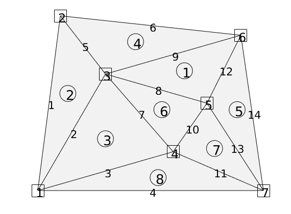
Output content of cells.faces, faces.nodes, and faces.neighbors to file
fp = fopen('G-unstructured.txt','w');
faces =[ rldecode(1 : G.cells.num,diff(G.cells.facePos), 2).' G.cells.faces];
fprintf(fp,'cells.faces =\n');
fprintf(fp,' %3d %3d\n', faces');
nodes = [ rldecode(1:G.faces.num,diff(G.faces.nodePos), 2).' G.faces.nodes];
fprintf(fp,'\n\nfaces.nodes =\n');
fprintf(fp,' %3d %3d\n', nodes');
fprintf(fp,'\n\nfaces.neighbors =\n');
fprintf(fp,' %3d %3d\n', G.faces.neighbors');
fclose(fp);
UNSTRUCTURED VORONOI
clf;
p = [ 0.0, 1.0, 1.0, 0.0, 0.0; ...
0.0, 0.0, 1.0, 1.0, 0.7]';
G = pebi(triangleGrid(p, delaunay(p(:,1),p(:,2))));
G = computeGeometry(G);
newplot;
plotGrid(G,'FaceColor',[0.95 0.95 0.95]); axis off;
%plotGrid(tri2grid( delaunay(p(:,1),p(:,2)), p), 'FaceColor','none','EdgeColor','r');
hold on;
% centroids
text(G.cells.centroids(:,1)-0.01, G.cells.centroids(:,2), ...
num2str((1:G.cells.num)'),'FontSize',20);
plot(G.cells.centroids(:,1), G.cells.centroids(:,2),...
'ok','MarkerSize',24);
% faces
text(G.faces.centroids(:,1)-0.02, G.faces.centroids(:,2)-0.01, ...
num2str((1:G.faces.num)'),'FontSize',16);
% vertices
text(G.nodes.coords(:,1)-0.02, G.nodes.coords(:,2)-0.005, ...
num2str((1:G.nodes.num)'),'FontSize',18);
plot(G.nodes.coords(:,1), G.nodes.coords(:,2),'sk','MarkerSize',24);
hold off;
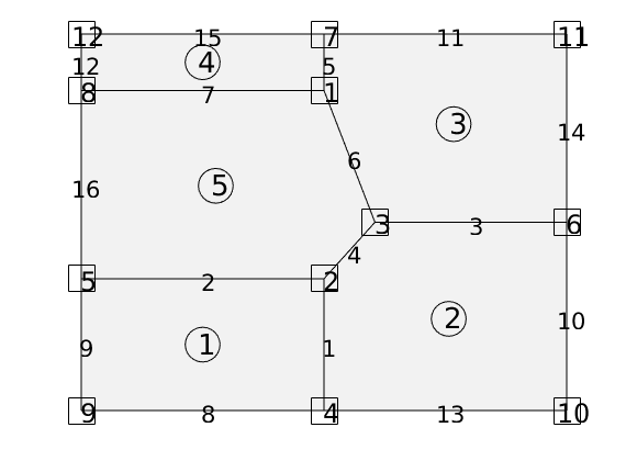
Output content of cells.faces, faces.nodes, and faces.neighbors to file
p = fopen('G-voronoi.txt','w');
faces =[ rldecode(1 : G.cells.num,diff(G.cells.facePos), 2).' G.cells.faces];
fprintf(fp,'cells.faces =\n');
fprintf(fp,' %3d %3d\n', faces');
nodes = [ rldecode(1:G.faces.num,diff(G.faces.nodePos), 2).' G.faces.nodes];
fprintf(fp,'\n\nfaces.nodes =\n');
fprintf(fp,' %3d %3d\n', nodes');
fprintf(fp,'\n\nfaces.neighbors =\n');
fprintf(fp,' %3d %3d\n', G.faces.neighbors');
fclose(fp);
[y,x,z] = peaks(15); z = z+8;
horizons = {struct('x',x,'y',y,'z',z),struct('x',x,'y',y,'z',z+8)};
grdecl = convertHorizonsToGrid(horizons,'layers', 4);
G = processGRDECL(grdecl);
figure, plotGrid(G); view(3); axis tight off
figure
surf(horizons{1}.x,horizons{1}.y,horizons{1}.z, 'EdgeC','r','FaceC',[.8 .8 .8]), hold on
mesh(horizons{2}.x,horizons{2}.y,horizons{2}.z, 'EdgeC','b','FaceC',[.7 .7 .7])
plot3([horizons{1}.x(:) horizons{2}.x(:)]',...
[horizons{1}.y(:) horizons{2}.y(:)]',...
[horizons{1}.z(:) horizons{2}.z(:)]',':k');
axis tight off, set(gca,'ZDir','reverse');
set(gca,'XLim',[-3.05 3.05]);
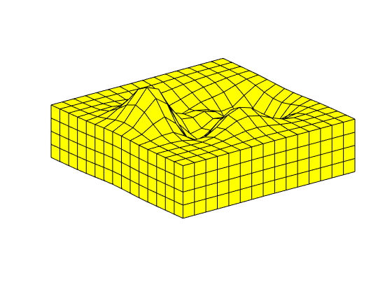
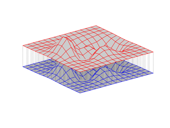
[n,m] = deal(30);
horizons = {struct('x',x,'y',y,'z',z),struct('x',x+.5,'y',2*y+1,'z',z+10)};
grdecl = convertHorizonsToGrid(horizons,'dims',[n m], 'layers', 3);
G = processGRDECL(grdecl);
figure
h1 = surf(horizons{1}.x,horizons{1}.y,horizons{1}.z-.1, ...
'EdgeC','r','FaceC',[.8 .8 .8]); hold on
h2 = mesh(horizons{2}.x,horizons{2}.y,horizons{2}.z, ...
'EdgeC','b','FaceC',[.7 .7 .7]);
xmin = min(cellfun(@(h) min(h.x(:)), horizons));
xmax = max(cellfun(@(h) max(h.x(:)), horizons));
ymin = min(cellfun(@(h) min(h.y(:)), horizons));
ymax = max(cellfun(@(h) max(h.y(:)), horizons));
[xi,yi] = ndgrid(linspace(xmin,xmax,n+1), linspace(ymin,ymax,m+1));
hi = mesh(xi,yi,26*ones(size(xi)),'FaceC','none');
hg = plotGrid(G);
hb1 = plot3(...
[-3 3 3 -3 -3 NaN -3 -3 NaN 3 3 NaN 3 3 NaN -3 -3], ...
[-3 -3 3 3 -3 NaN -3 -3 NaN -3 -3 NaN 3 3 NaN 3 3],...
[26 26 26 26 26 NaN 26 8 NaN 26 8 NaN 26 8 NaN 26 8],'r-','LineWidth',2);
hb2 = plot3(...
[-2 4 4 -2 -2 NaN -2 -2 NaN 4 4 NaN 4 4 NaN -2 -2]-.5, ...
[-5 -5 7 7 -5 NaN -5 -5 NaN -5 -5 NaN 7 7 NaN 7 7],...
[26 26 26 26 26 NaN 26 18 NaN 26 18 NaN 26 18 NaN 26 18],'b-','LineWidth',2);
axis tight off, view(-140,30)
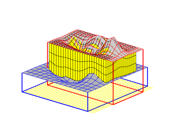
Hierarchical Coarsening
Generated from showHierCoarsen.m
This is a relatively simple example that illustrates the basic idea behind hierarchical coarsening. The model has two geological properties, unit and lithofacies assemblage (LFA), that are used to generate permeability. These two partitions are applied recursively together with a nested set of uniform partitions with permeability as an indicator.
mrstModule add coarsegrid agglom
% Load facies data
exdir = fullfile(mrstPath('agglom'), 'examples');
imload = @(fn) ...
flipud(double(sum(imread(fullfile(exdir, 'data', fn)), 3))) .';
f = imload('facies1.png'); f(2,16)=max(f(:));
pl = 3-compressPartition(f(:) + 1);
% Create grid
G = computeGeometry(cartGrid(size(f))); clear f;
x = G.cells.centroids;
% Make unit data
pu = (x(:,2)>15+0.25*x(:,1))+1;
% Make fault blocks
faults = [12:42:29*42 1692:41:2840 432:41:1630];
pf = processPartition(G, ones(G.cells.num,1), faults);
% Generate and plot a simple permeability model
rng(1000);
K = 1 + (pl-1)*8+.3*pu.*randn(G.cells.num,1); I = K-min(K)+.1;
figure(1); clf,
plotCellData(G,I,'EdgeColor','none');
axis equal off; colormap(.8*jet(128)+.2*ones(128,3))
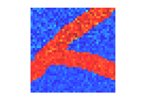
Apply the geological features recursively
In addition to the geological features, we create a hierarchy of refined partitions that will be used to further subdivide the high-permeable LFA
pc = ones(G.cells.num,3);
for i=1:4
pc(:,i) = partitionCartGrid(G.cartDims,[5 5].*2^(i-1));
end
p = applySuccessivePart(processPartition(G,pu,faults),G, I, 8, [pl pc]);
% Visualize results
figure(2); clf, set(gcf,'Position',[670 490 760 470]);
subplot(2,3,1)
plotCellData(G, pl, 'EdgeColor','none'); axis equal off
subplot(2,3,2);
plotCellData(G, pu, 'EdgeColor','none'); axis equal off
subplot(2,3,3)
plotCellData(G, pl+2*(pu-1), 'EdgeColor','none'); axis equal off
plotFaces(G, faults,'EdgeColor','k','LineWidth',1)
subplot(2,3,5); cla
plotCellData(G, pl+2*(pu-1),'EdgeColor','none'); axis equal off
outlineCoarseGrid(G, p, 'k','LineWidth',1);
colormap([.5 .5 1; .2 .2 .8; .3 .6 .6; .1 .4 .4]);
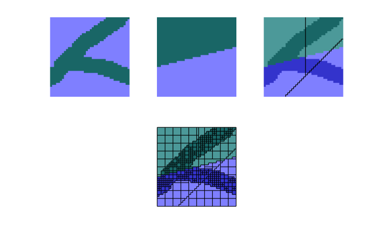
Merge small blocks outside of high-permeable lithofacies
We merge all blocks that have three cells or less in the first LFA, which is assumed to have less permeability than the second lithofacies. To this end, we remove cell connections within LFA two as well as connections across different units, lithofacies, and faults.
subplot(2,3,6), cla
plotCellData(G, pl+2*(pu-1),'EdgeColor','none'); axis equal off
qb = [0; processPartition(G,pl+2*(pu-1), faults)];
ql = [0; pl];
T = 2*(qb(G.faces.neighbors(:,1)+1)==qb(G.faces.neighbors(:,2)+1))-1;
T(ql(G.faces.neighbors(:,1)+1)==2) = -1;
pm = mergeBlocksByConnections(G, p, T, 4);
outlineCoarseGrid(G,pm, 'k','LineWidth',1);
for i=[1:3 5:6],
subplot(2,3,i),
set(gca,'Position',get(gca,'Position')+[-.025 -.025 .05 .05]);
end
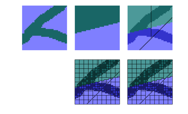
Example 1: Cartesian grid with radial refinement
Generated from showHybridGrids.m
Pw = [];
for r = exp(-3.5:.2:0),
[x,y,z] = cylinder(r,28); Pw = [Pw [x(1,:); y(1,:)]];
end
Pw = [Pw [0; 0]];
Pw1 = bsxfun(@plus, Pw, [2; 2]);
Pw2 = bsxfun(@plus, Pw, [12; 6]);
[x,y] = meshgrid(0:.5:14, 0:.5:8);
P = unique([Pw1'; Pw2'; x(:) y(:)], 'rows');
G = pebi(triangleGrid(P));
plotGrid(G);
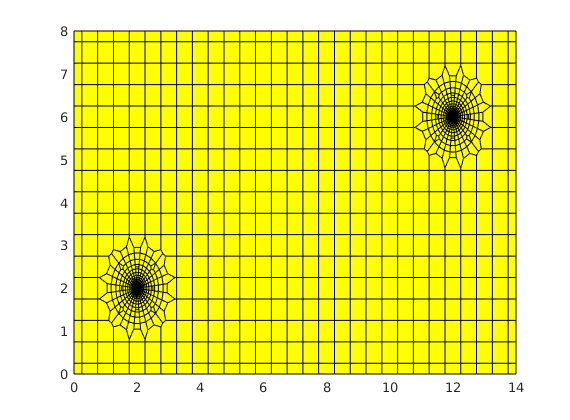
Example 1: Cartesian grid with refinement in the middle
Generated from showMultiBlockGrid.m
clf
G1 = cartGrid([ 4 4],[1 1]);
G2 = cartGrid([ 8 8],[1 1]);
G3 = cartGrid([12 4],[3 1]);
% Glue middle part
G1 = translateGrid(G1,[0 1]); plotGrid(G1,'FaceColor',[1 .9 .9]);
G2 = translateGrid(G2,[1 1]); plotGrid(G2,'FaceColor',[.9 1 .9]);
G = glue2DGrid(G1, G2);
G1 = translateGrid(G1,[2 0]); plotGrid(G1,'FaceColor',[1 .9 .9]);
G = glue2DGrid(G, G1);
% Glue top and bottom
G = glue2DGrid(G, G3); plotGrid(G3,'FaceColor',[.9 .9 1]);
G3 = translateGrid(G3,[0 2]); plotGrid(G3,'FaceColor',[.9 .9 1]);
G = glue2DGrid(G3, G); %#ok<NASGU>
%print -depsc2 multiBlock-1a.eps;
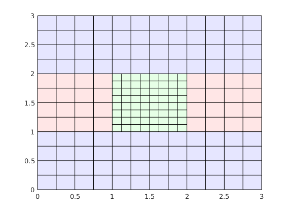
Repeat the whole process without intermediate plotting
G1 = cartGrid([ 5 5],[1 1]);
G2 = cartGrid([20 20],[1 1]);
G3 = cartGrid([15 5],[3 1]);
G = glue2DGrid(G1, translateGrid(G2,[1 0]));
G = glue2DGrid(G, translateGrid(G1,[2 0]));
G = glue2DGrid(G3, translateGrid(G, [0 1]));
G = glue2DGrid(G, translateGrid(G3,[0 2]));
G = twister(G);
clf
plotGrid(G,'FaceColor','none');
%print -depsc2 multiBlock-1b.eps;
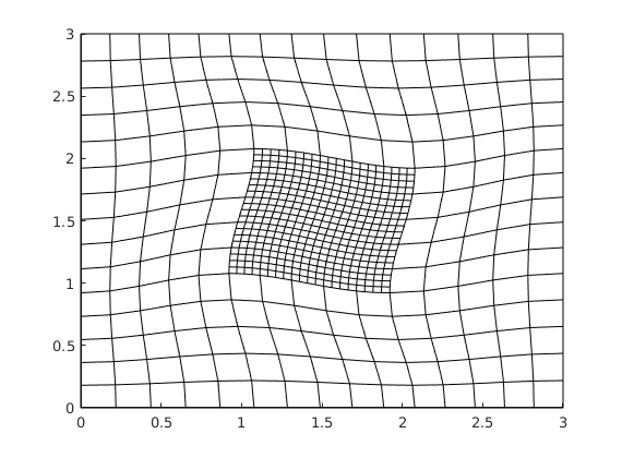
Example 2: Cartesian grid with triangular/PEBI refinement
Construct unstructured grid
[N,M]=deal(10,15);
xv = linspace(0,1,N+1);
yv = linspace(0,1,M+1);
[x,y] = ndgrid(xv, yv);
x(2:N,2:M) = x(2:N,2:M) + 0.3*randn(N-1,M-1)*max(diff(xv));
y(2:N,2:M) = y(2:N,2:M) + 0.3*randn(N-1,M-1)*max(diff(yv));
G2 = computeGeometry(triangleGrid([x(:) y(:)]));
% Set orientation of faces
hf = G2.cells.faces(:,1);
hf2cn = gridCellNo(G2);
sgn = 2*(hf2cn == G2.faces.neighbors(hf, 1)) - 1;
N = bsxfun(@times, sgn, G2.faces.normals(hf,:));
N = bsxfun(@rdivide, N, G2.faces.areas(hf,:));
n = zeros(numel(hf),2); n(:,1)=1;
% Add cell tags
G2.cells.faces(:,2) = zeros(size(hf));
i = sum(N.*n,2)==-1; G2.cells.faces(i,2) = 1;
i = sum(N.*n,2)== 1; G2.cells.faces(i,2) = 2;
n = n(:,[2 1]);
i = sum(N.*n,2)==-1; G2.cells.faces(i,2) = 3;
i = sum(N.*n,2)== 1; G2.cells.faces(i,2) = 4;
% Glue grids together
G = glue2DGrid(G1, translateGrid(G2,[1 0]));
G = glue2DGrid(G, translateGrid(G1,[2 0]));
G = glue2DGrid(G3, translateGrid(G, [0 1]));
G = glue2DGrid(G, translateGrid(G3,[0 2]));
G = twister(G);
clf
plotGrid(G,'FaceColor','none');
%print -depsc2 multiBlock-2a.eps;
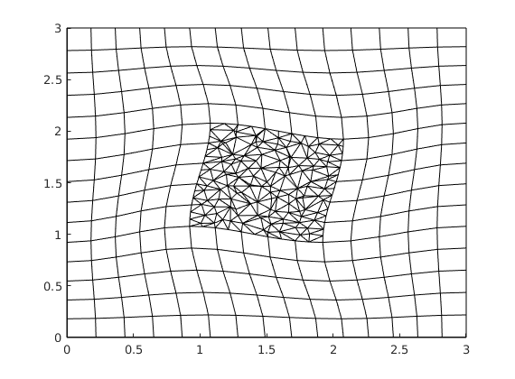
Repeat with Voronoi grid instead
[N,M]=deal(8,12);
xv = linspace(0,1,N+1);
yv = linspace(0,1,M+1);
[x,y] = ndgrid(xv, yv);
x(2:N,2:M) = x(2:N,2:M) + 0.3*randn(N-1,M-1)*max(diff(xv));
y(2:N,2:M) = y(2:N,2:M) + 0.3*randn(N-1,M-1)*max(diff(yv));
G2 = computeGeometry(pebi(triangleGrid([x(:) y(:)])));
% Set orientation of faces
hf = G2.cells.faces(:,1);
hf2cn = gridCellNo(G2);
sgn = 2*(hf2cn == G2.faces.neighbors(hf, 1)) - 1;
N = bsxfun(@times, sgn, G2.faces.normals(hf,:));
N = bsxfun(@rdivide, N, G2.faces.areas(hf,:));
n = zeros(numel(hf),2); n(:,1)=1;
G2.cells.faces(:,2) = zeros(size(hf));
i = sum(N.*n,2)==-1; G2.cells.faces(i,2) = 1;
i = sum(N.*n,2)== 1; G2.cells.faces(i,2) = 2;
n = n(:,[2 1]);
i = sum(N.*n,2)==-1; G2.cells.faces(i,2) = 3;
i = sum(N.*n,2)== 1; G2.cells.faces(i,2) = 4;
% Refine G3 in the x-direction and rescale in y-direction
G3 = cartGrid([24 5], [3 .25]);
G = glue2DGrid(G1, translateGrid(G2,[1 0]));
G = glue2DGrid(G, translateGrid(G1,[2 0]));
G = glue2DGrid(G3, translateGrid(G, [0 .25]));
G = glue2DGrid(G, translateGrid(G3,[0 1.25]));
G = twister(G);
clf
plotGrid(G,'FaceColor','none');
%print -depsc2 multiBlock-2b.eps;
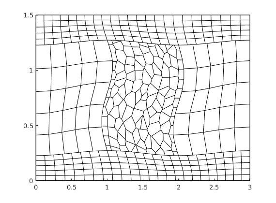
Example 3: Extruded grid rotated
G = glue2DGrid(G1, translateGrid(G2,[0 1]));
G = glue2DGrid(G, translateGrid(G1,[0 2]));
G = makeLayeredGrid(G, 5);
G.nodes.coords = G.nodes.coords(:,[3 1 2]);
clf, plotGrid(G,'FaceColor',[1 1 1]); view(115,20); axis off
%print -depsc2 multiBlock-3.eps;
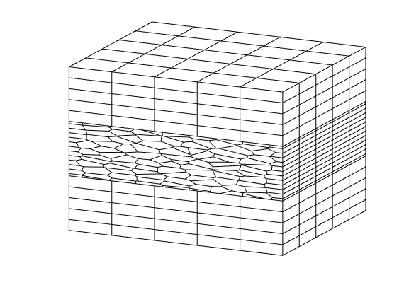
Examples of Voronoi / Perpendicular Bisector (PEBI) grids
Generated from showPEBI.m
In this script, we go through several examples of polyhedral grids in 3D.
Plot of Voronoi grid + pillars
[x,y] = meshgrid((0:2)*2*cos(pi/6),0:2);
x = [x(:); x(:)+cos(pi/6)];
y = [y(:); y(:)+sin(pi/6)];
a = [0 4.3 0 2.5 0 1.5];
clf
plot3(x,y,zeros(size(x)),'o'); view(40,30); axis tight off;
T = triangleGrid([x(:),y(:)]);
T.nodes.coords(:,3) = zeros(size(T.nodes.coords(:,1)));
plotGrid(T,'FaceColor','none'); view(40,30);
axis(a); axis equal tight off;
set(gca,'zdir','normal');
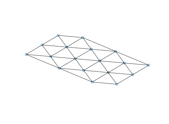
G = pebi(T);
G.nodes.coords(:,3) = zeros(size(G.nodes.coords(:,1)));
plotGrid(G,'FaceColor','none','EdgeColor','r'); set(gca,'zdir','normal');
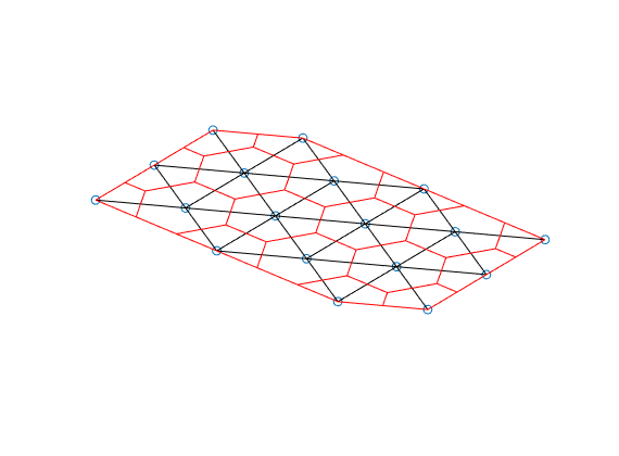
newplot
plotGrid(G, 'FaceColor',[.9 .4 .4]); axis(a); axis off
hold on
G1 = G;
G1.nodes.coords(:,3) = 1.5;
G1.nodes.coords(:,1:2) = 0.925*G.nodes.coords(:,1:2);
plot3([G.nodes.coords(:,1) G1.nodes.coords(:,1)]', ...
[G.nodes.coords(:,2) G1.nodes.coords(:,2)]', ...
[G.nodes.coords(:,3) G1.nodes.coords(:,3)]', '-k','LineWidth',1);
set(gca,'zdir','normal'); view(40,30),
axis(a), axis equal tight off
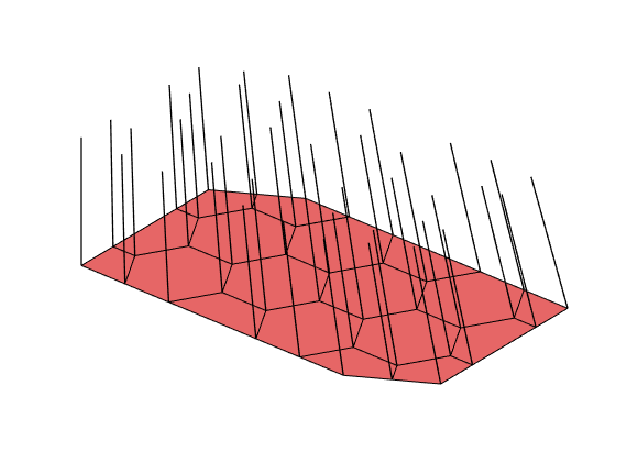
G1 = G;
G1.nodes.coords(:,3) = 1;
G1.nodes.coords(:,1:2) = 0.95*G1.nodes.coords(:,1:2);
plotGrid(G1, 'FaceColor',[.4 .4 .9]); set(gca,'zdir','normal');
hold off
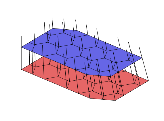
Make a good radial grid
newplot
P = [];
for r = exp(-3.5:0.25:0),
[x,y,z] = cylinder(r,10); P = [P [x(1,:); y(1,:)]]; %#ok<AGROW>
end
P = unique(P','rows');
G = makeLayeredGrid(pebi(triangleGrid(P)), 5);
plotGrid(G,'FaceColor',[.8 .8 .8]); view(30,50), axis tight off
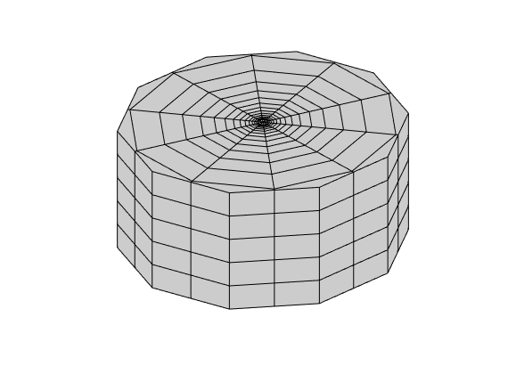
Make a grid draped over peaks
x,y] = meshgrid((0:6)*2*cos(pi/6),0:7);
x = [x(:); x(:)+cos(pi/6)]; x=(x - mean(x(:)))/2;
y = [y(:); y(:)+sin(pi/6)]; y=(y - mean(y(:)))/2;
G = pebi(triangleGrid([x(:),y(:)]));
G.nodes.coords(:,3) = -peaks(G.nodes.coords(:,1),G.nodes.coords(:,2));
clf,
plotGrid(G); view(25,50), axis tight off
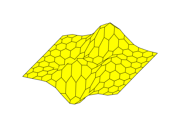
How to Partition Grids
Generated from showPartitions.m
In this script, we go through several examples that demonstrate various methods for partitioning grids using MRST
mrstModule add coarsegrid
Partition a Cartesian 2D grid
We use partitionUI which exploits the logical structure and creates a uniform grid in logical space.
figure
G = cartGrid([7,7]);
p = partitionUI(G, [2,2]);
plotCellData(G, p, 'EdgeColor', 'y');
outlineCoarseGrid(G, p, 'k');
axis tight off,
caxis([.5 max(p)+.5]);
colormap(0.5*(lines(max(p))+ones(max(p),3)));
set(colorbar,'YTick',1:max(p));
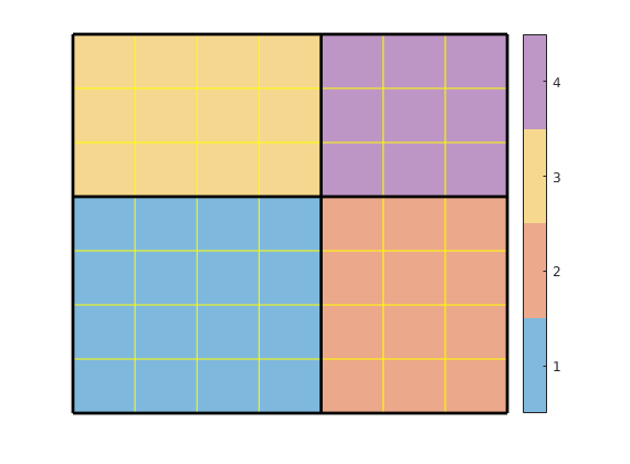
Partition a 3D grid in much the same manner
figure
G = cartGrid([10,10,4]);
p = partitionUI(G, [3,3,2]);
plotCellData(G, p, 'Edgecolor', 'w');
outlineCoarseGrid(G, p, 'EdgeColor','k','lineWidth',4);
colormap(.5*(colorcube(max(p)) + ones(max(p),3)));
view(3);
axis off
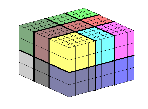
Partition according to polar coordinate
figure
G = cartGrid([11, 11],[2,2]);
G.nodes.coords = ...
bsxfun(@minus, G.nodes.coords, 1);
G = computeGeometry(G);
c = G.cells.centroids;
[th,r] = cart2pol(c(:,1),c(:,2));
p = mod(round(th/pi*4)+4,4)+1;
p(r<.3) = max(p)+1;
% Plot partition
plotCellData(G,p,'EdgeColor',[.7 .7 .7]);
outlineCoarseGrid(G,p,'k');
caxis([.5 max(p)+.5]);
colormap(.5*(jet(max(p))+ones(max(p),3)));
set(colorbar,'YTick',1:max(p),'FontSize',16);
axis off
% Split blocks that are multiply connected into a set of singly connected
% blocks and plot the new partition
p = processPartition(G, p);
figure
plotCellData(G,p,'EdgeColor',[.7 .7 .7]);
outlineCoarseGrid(G,p,'k');
caxis([.5 max(p)+.5]);
colormap(.5*(jet(max(p))+ones(max(p),3)));
set(colorbar,'YTick',1:max(p),'FontSize',16);
axis off
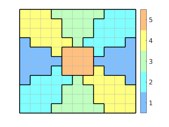
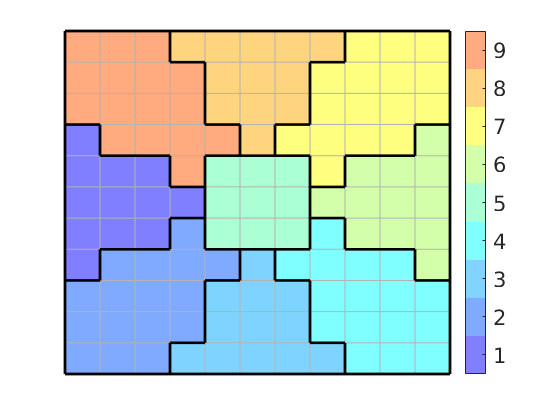
Combine a facies and a Cartesian partition
clear
G = cartGrid([20, 20], [1 1]);
G = computeGeometry(G);
f = @(c) sin(4*pi*(c(:,1)-c(:,2)));
pf = 1 + (f(G.cells.centroids) > 0);
pc = partitionCartGrid(G.cartDims, [4 4]);
% Alternative 1:
[b,~,p] = unique([pf, pc], 'rows' );
% Alternative 2:
q = compressPartition(pf + max(pf)*pc); %#ok<NASGU>
% Plot results
figure
plotCellData(G,p);
outlineCoarseGrid(G, p, 'k','LineWidth',2);
axis off
colormap(.5*(jet(64)+ones(64,3)))
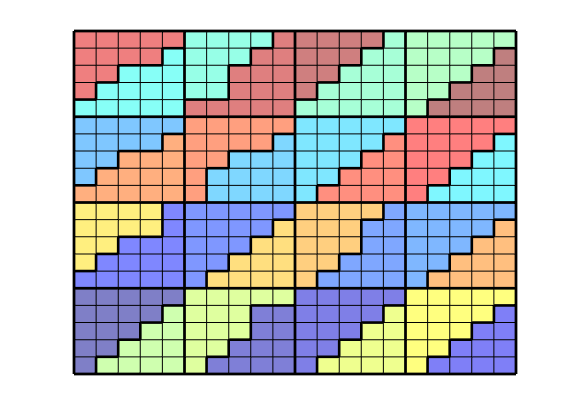
Partition a cup-formed grid
igure
x = linspace(-2,2,41);
G = tensorGrid(x,x,x);
G = computeGeometry(G);
c = G.cells.centroids;
r = c(:,1).^2 + c(:,2).^2+c(:,3).^2;
G = removeCells(G, (r>1) | (r<0.25) | (c(:,3)<0));
plotGrid(G); view(15,60); axis tight off
% Make the partition vector contiguous:
figure
p = partitionUI(G,[5 5 4]);
subplot(2,1,1); bar(accumarray(p,1)); shading flat
q = compressPartition(p);
subplot(2,1,2); bar(accumarray(q,1)); shading flat
set(gca,'XLim',[0 100]);
% Visualize the partition using an exploding view
figure
explosionView(G,q,.4);
view(15,60); axis tight off
colormap(colorcube(max(q)));
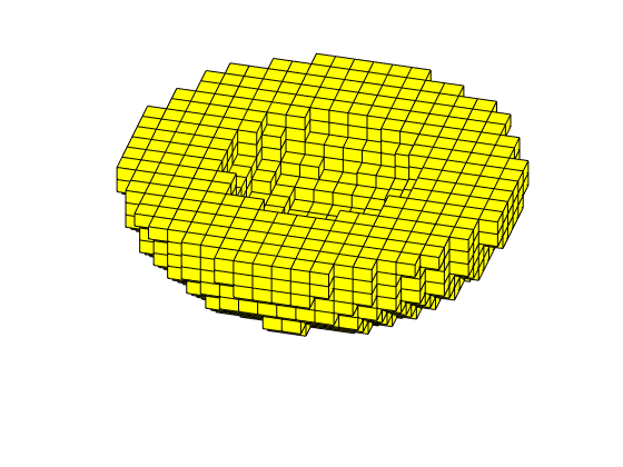
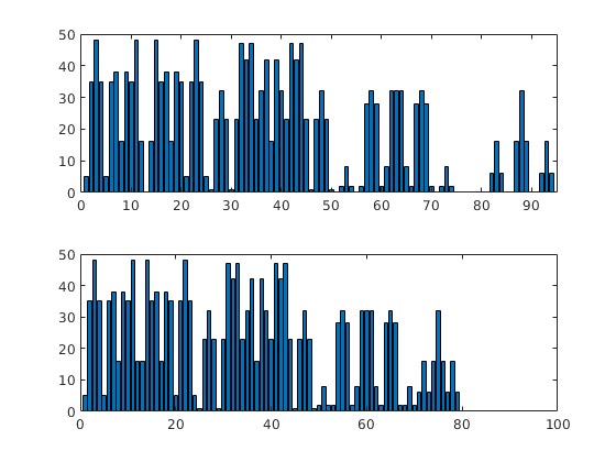
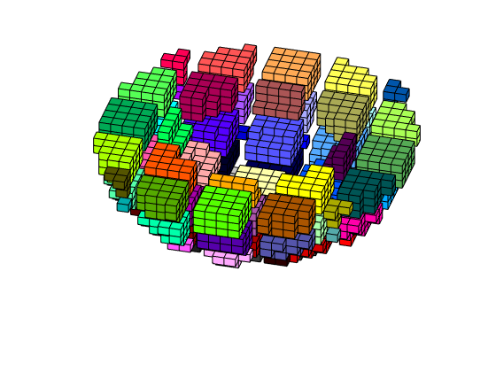
grdecl = simpleGrdecl([4, 2, 3], .12, 'flat', true);
[X,Y,Z] = buildCornerPtPillars(grdecl,'Scale',true);
[x,y,z] = buildCornerPtNodes(grdecl);
Plot pillars
Generated from showPillarGrid.m
plot3(X',Y',Z','k'); drawAxisCross(.15); axis tight;
set(gca,'zdir','reverse'), view(35,35), axis off, zoom(1.2);
set(gca,'dataaspectRatio',[1.8,1.8,1])
set(gca,'Clipping','off')
% print -deps2 showCPgrid-pillars.eps;
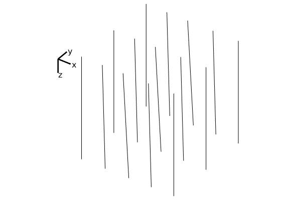
Plot points on pillars, mark pillars with faults red
hold on; I=[3 8 13];
hpr = plot3(X(I,:)',Y(I,:)',Z(I,:)','r','LineWidth',2);
hpt = plot3(x(:),y(:),z(:),'o');
hold off;
% print -depsc2 showCPgrid-pts.eps;
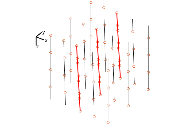
Create grid and plot two stacks of cells
G = processGRDECL(grdecl);
args = {'FaceColor'; 'r'; 'EdgeColor'; 'k'};
hcst = plotGrid(G,[1:8:24 7:8:24],'FaceAlpha', .1, args{:});
% print -dpng showCPgrid-cells.png;
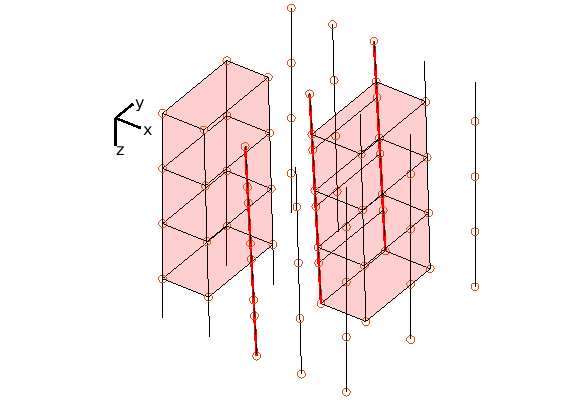
Plot cells and fault surface
elete([hpt; hpr; hcst]);
plotGrid(G,'FaceAlpha', .15, args{:});
plotFaces(G, G.faces.tag>0,'FaceColor','b','FaceAlpha',.4);
% print -dpng showCPgrid-grid.png;
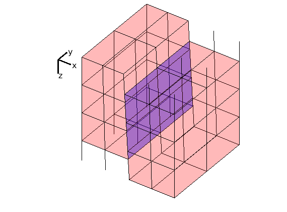
load(fullfile('data','showProcessPartition.mat'));
Plot grid
Generated from showProcessPartition.m
figure, plotGrid(G,c,'FaceColor',0.7*col+[.3 .3 .3]);
text(G.cells.centroids(c,1), G.cells.centroids(c,2),...
num2str((1:numel(c))'),'HorizontalAlignment','center','FontSize',20);
axis off tight
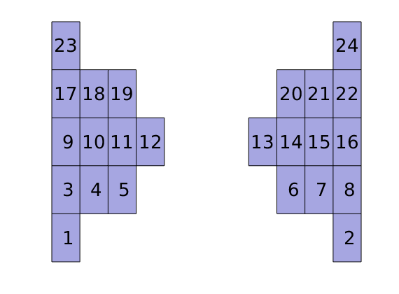
Plot original adjacency matrix
figure,
val = ones(size(c));
val(p(1:r(2)-1))=1; val(p(r(2):r(3)-1))=2;
hold on;
i1 = val(ii)==1; plot(ii(i1),jj(i1),'or','MarkerSize',6,'MarkerFaceColor','r');
i2 = val(ii)==2; plot(ii(i2),jj(i2),'ob','MarkerSize',6,'MarkerFaceColor','b');
set(gca,'YDir','reverse','FontSize',14); axis square tight
hold off
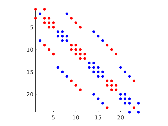
Plot permuted adjacency matrix
figure,
n(p) = 1:numel(c);
hold on;
plot(n(ii(i1)),n(jj(i1)),'or','MarkerSize',6,'MarkerFaceColor','r');
plot(n(ii(i2)),n(jj(i2)),'ob','MarkerSize',6,'MarkerFaceColor','b');
plot([12.5 12.5 NaN .5 24.5],[.5 24.5 NaN 12.5 12.5],'--k');
set(gca,'YDir','reverse','FontSize',14); axis square tight
hold off
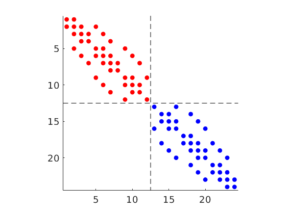
Simple 2D Cartesian grids
Generated from showStructGrids.m
show a graded grid
clf;
dx = 1-0.5*cos((-1:0.1:1)*pi); x = -1.15+0.1*cumsum(dx);
y = 0:0.05:1;
G = tensorGrid(x, sqrt(y));
plotGrid(G); axis([-1.05 1.05 -0.05 1.05]);
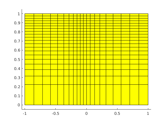
Random perturbations
clf;
nx = 6; ny=12;
G = cartGrid([nx, ny]); subplot(1,2,1); plotGrid(G);
c = G.nodes.coords;
I = or( or(any(c==0,2), any(c(:,1)==nx,2)), any(c(:,2)==ny,2));
G.nodes.coords(~I,:) = c(~I,:) + 0.6*rand(sum(~I),2)-0.3;
subplot(1,2,2); plotGrid(G);
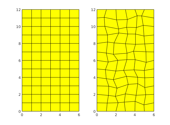
Example grid: twister
clf;
G = cartGrid([30, 20]);
G.nodes.coords = twister(G.nodes.coords);
G = computeGeometry(G);
plotCellData(G, G.cells.volumes, 'EdgeColor', 'k'), colorbar
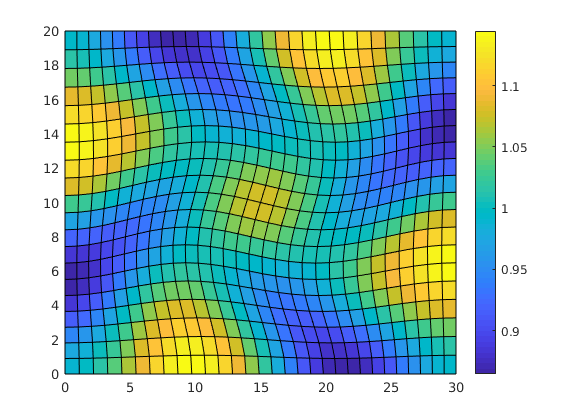
removeCells: Create an ellipsoid grid
lf;
x = linspace(-2,2,21);
G = tensorGrid(x,x,x);
subplot(1,2,1); plotGrid(G);view(3); axis equal
subplot(1,2,2); plotGrid(G,'FaceColor','none','LineWidth',0.01);
G = computeGeometry(G);
c = G.cells.centroids;
r = c(:,1).^2 + 0.25*c(:,2).^2+0.25*c(:,3).^2;
G = removeCells(G, find(r>1));
plotGrid(G); view(-70,70); axis equal
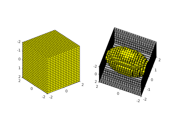
Tessellations of 2D space
Generated from showTessellation.m
We consider a set of different examples of tessellations of increasing complexity. The first is just a standard Cartesian grid based on a regular quadrilaterals. The next three are n-polygonal extensions of a regular triangular tessellation.
colormap(.6*parula(128)+.4*ones(128,3));

Example 1: Cartesian grid
This grid is formed by laying out regular quadrilaterals
[nx,ny] = deal(15,10);
[x,y] = meshgrid(linspace(0,1,nx+1),linspace(0,1,ny+1));
p = [x(:) y(:)];
n = (nx+1)*(ny+1);
I = reshape(1:n,ny+1,nx+1);
T = [
reshape(I(1:end-1,1:end-1),[],1)';
reshape(I(1:end-1,2:end ),[],1)';
reshape(I(2:end, 2:end ),[],1)';
reshape(I(2:end, 1:end-1),[],1)'
]';
G = tessellationGrid(p, T);
clf, plotGrid(G);
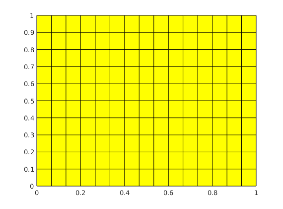
Example 2: convex/concave hexagonal tiles
We first generate the two hexagonal tiles. Then, we identify three symmetry lines (that together make up a triangle for each tile) and use these to fit the tiles together in space.
% Construct two symmetric convex/concave hexagonal tiles
[dx, dy, dPhi] = deal(cos(pi/3),sin(pi/3), pi*15/180);
v = pi/180*[0 120 240]';
dv = [cos(v-dPhi) sin(v-dPhi) cos(v+dPhi) sin(v+dPhi)]/2;
P = [ 0 0 0 0;
0+dv(1,1) 0+dv(1,2) 0+dv(1,3) 0+dv(1,4);
1 0 1 0;
1+dv(2,1) 0+dv(2,2) 1+dv(2,3) 0+dv(2,4);
dx dy dx dy;
dx+dv(3,1) dy+dv(3,2) dx+dv(3,3) dy+dv(3,4)];
P1 = P(:,1:2);
P2 = [P([1 6:-1:2],3) -P([1 6:-1:2],4)];
clf
plotCellData(tessellationGrid([P1; P2], reshape(1:12,6,2)'),(1:2)',...
'EdgeColor','k');
% Add help triangles that give the symmetry-directions we will use to fit
% the tiles together
P = [0 0; 1 0; dx dy];
Gt = triangleGrid([P; P([1 3 2],1), -P([1 3 2],2)],reshape(1:6,3,2)');
plotGrid(Gt,'FaceColor','none'); axis equal off;
plotGrid(Gt,'FaceColor','none','LineWidth',2);
axis equal off
% print -depsc2 convexConcave-1.eps;
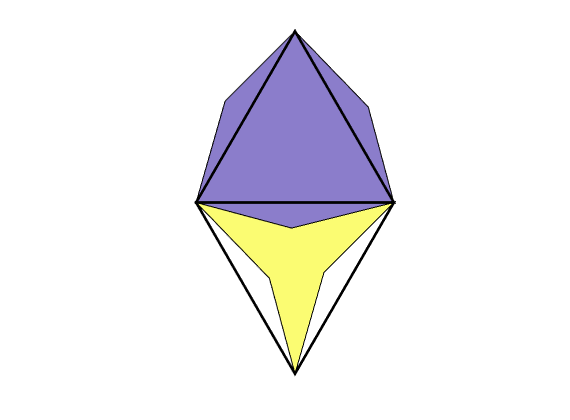
To make a full tiling, we make a basic pattern consisting of four triangles and then use this pattern to tile as much of space as we want
[p,t,n] = deal([],[],0);
T = reshape(1:24,6,4)';
for j=0:1
for i=0:3
p = [p; bsxfun(@plus,P1,[i 2*j*dy])]; %#ok<AGROW>
p = [p; bsxfun(@plus,P2,[i-dx (2*j+1)*dy])]; %#ok<AGROW>
p = [p; bsxfun(@plus,P1,[i-dx (2*j+1)*dy])]; %#ok<AGROW>
p = [p; bsxfun(@plus,P2,[i 2*(j+1)*dy])]; %#ok<AGROW>
t = [t; T+n]; n=n+24; %#ok<AGROW>
end
end
[p,~,ic] = unique(round(p*1e5)/1e5,'rows');
G = tessellationGrid(p, ic(t));
i=repmat((1:2)',G.cells.num/2,1);
clf; plotCellData(G,i(:));
%plotFaces(G,find(any(G.faces.neighbors==0,2)),'EdgeColor','r','LineWidth',2);
axis equal tight off; drawnow
% print -depsc2 convexConcave-2.eps;
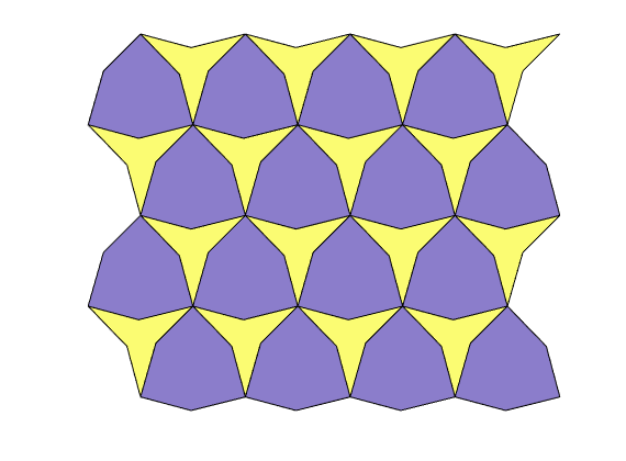
Example 3: nonagonal tiles
Using the same approach as in the previous example, we can make a set of nonagonal tiles
[dx, dy, dPhi] = deal(cos(pi/3),sin(pi/3), pi*40/180);
v = pi/180*[0 180 120 -60 240 60]';
dv = [cos(v-dPhi) sin(v-dPhi) cos(v+dPhi) sin(v+dPhi)]/3.5;
P = [...
0 0 0 0;
0+dv(1,1) 0+dv(1,2) 0+dv(1,3) 0+dv(1,4);
1+dv(2,1) 0+dv(2,2) 1+dv(2,3) 0+dv(2,4);
1 0 1 0;
1+dv(3,1) 0+dv(3,2) 1+dv(3,3) 0+dv(3,4);
dx+dv(4,1) dy+dv(4,2) dx+dv(4,3) dy+dv(4,4);
dx dy dx dy;
dx+dv(5,1) dy+dv(5,2) dx+dv(5,3) dy+dv(5,4);
0+dv(6,1) 0+dv(6,2) 0+dv(6,3) 0+dv(6,4);
];
m = size(P,1);
P1 = P(:,1:2);
P2 = [P([1 m:-1:2],3) -P([1 m:-1:2],4)];
T = reshape(1:4*m,m,4)';
[p,t,n] = deal([],[],0);
for j=0:2
for i=0:4
p = [p; bsxfun(@plus,P1,[i 2*j*dy])]; %#ok<AGROW>
p = [p; bsxfun(@plus,P2,[i-dx (2*j+1)*dy])]; %#ok<AGROW>
p = [p; bsxfun(@plus,P1,[i-dx (2*j+1)*dy])]; %#ok<AGROW>
p = [p; bsxfun(@plus,P2,[i 2*(j+1)*dy])]; %#ok<AGROW>
t = [t; T+n]; n=n+4*m; %#ok<AGROW>
end
end
[p,ia,ic] = unique(round(p*1e5)/1e5,'rows');
G = tessellationGrid(p, ic(t));
i=repmat((1:2)',G.cells.num/2,1);
clf
plotCellData(G,i(:));
%plotFaces(G,find(any(G.faces.neighbors==0,2)),'LineWidth',2);
axis tight off;
Example 4: pentadecagonal tiles
In this example, we use a slightly different approach. We first create a regular triangular tiling, and then we go through the line segments of the triangles and add one by one point
% Basic patterns consisting of uniform triangles
[dx, dy] = deal(cos(pi/3),sin(pi/3));
P1 = [0 0; 1 0; dx dy];
P2 = [P1([1 3 2],1) -P1([1 3 2],2)];
[p,t,n] = deal([],[],0);
for j=0:1
for i=0:3
p = [p; bsxfun(@plus,P1,[i 2*j*dy])]; %#ok<AGROW>
p = [p; bsxfun(@plus,P2,[i-dx (2*j+1)*dy])]; %#ok<AGROW>
p = [p; bsxfun(@plus,P1,[i-dx (2*j+1)*dy])]; %#ok<AGROW>
p = [p; bsxfun(@plus,P2,[i 2*(j+1)*dy])]; %#ok<AGROW>
t = [t; [1:3; 4:6; 7:9; 10:12]+n]; n=n+12; %#ok<AGROW>
end
end
%{
% In case you just want to show two polygons as in the book
p = [P1; P2];
t = reshape(1:6,3,2)';
%}
We then extract the end-points on each edge and compute the angle the corresponding line makes with the x-axis. We will use this information to perturb the points. By using this orientation of the lines, we can easily make sure that the perturbations are introduced in the correct direction.
dPhi = pi*35/180;
e = reshape(t(:,[1 2 2 3 3 1])',2,[])';
v = p(e(:,2),:) - p(e(:,1),:);
phi = atan2(v(:,2),v(:,1));
P = p;
T = reshape(e',6,[])';
T = T(:,[1 3 5]);
[Pp,~,ic] = unique(round(P*1e5)/1e5, 'rows','stable');
G = tessellationGrid(Pp,ic(T));
i=repmat((1:2)',G.cells.num/2,1);
clf
plotCellData(G,i(:));
axis equal off
% print -depsc2 trigon.eps;
Add the first set of points, making an irregular hexagonal tile
pn = p(e(:,1),:) + 1/3*[cos(phi-dPhi) sin(phi-dPhi)];
e = e(:,[1 1 2]);
e(:,2) = size(P,1)+(1:size(pn,1)).';
P = [P; pn];
T = reshape(e',9,[])';
T = T(:,[1:2 4:5 7:8]);
[Pp,~,ic] = unique(round(P*1e5)/1e5, 'rows','stable');
G = tessellationGrid(Pp,ic(T));
i=repmat((1:2)',G.cells.num/2,1);
clf
plotCellData(G,i(:));
axis equal off
% print -depsc2 hexagon.eps;
Reshape into irregular nonagons
pn = p(e(:,1),:) + 1/3*[cos(phi-.2*dPhi) sin(phi-.2*dPhi)];
e = e(:,[1:3 3]);
e(:,3) = size(P,1)+(1:size(pn,1)).';
P = [P; pn];
T = reshape(e',12,[])';
T = T(:,[1:3 5:7 9:11]);
[Pp,~,ic] = unique(round(P*1e5)/1e5, 'rows','stable');
G = tessellationGrid(Pp,ic(T));
i=repmat((1:2)',G.cells.num/2,1);
clf
plotCellData(G,i(:));
axis equal off
% print -depsc2 nonagon.eps;
Reshape into irregular dodecagons
phi = atan2(-v(:,2),-v(:,1));
pn = p(e(:,4),:) + 1/3*[cos(phi-.2*dPhi) sin(phi-.2*dPhi)];
e = e(:,[1:4 4]);
e(:,4) = size(P,1)+(1:size(pn,1)).';
P = [P; pn];
T = reshape(e',15,[])';
T = T(:,[1:4 6:9 10:14]);
[Pp,~,ic] = unique(round(P*1e5)/1e5, 'rows','stable');
G = tessellationGrid(Pp,ic(T));
i=repmat((1:2)',G.cells.num/2,1);
clf
plotCellData(G,i(:));
axis equal off
% print -depsc2 dodecagon.eps;
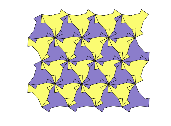
Reshape into irregular pentadecagon
e = e(:,[1:5 5]);
pn = p(e(:,5),:) + 1/3*[cos(phi-dPhi) sin(phi-dPhi)];
e(:,5) = size(P,1)+(1:size(pn,1)).';
P = [P; pn];
T = reshape(e',18,[])';
T = T(:,[1:5 7:11 13:17]);
[P,~,ic] = unique(round(P*1e5)/1e5, 'rows','stable');
G = tessellationGrid(P,ic(T));
i=repmat((1:2)',G.cells.num/2,1);
clf
plotCellData(G,i(:));
axis equal off;
% print -depsc2 pentadecagon.eps;

%{
Triangulation of a set of random points
Generated from showTriangularGrids.m
clf
p = rand(10,2);
t = delaunayn(p);
G = triangleGrid(p,t);
plotGrid(G,'FaceColor','none');
hold on; plot(p(:,1),p(:,2),'o'); hold off; axis off;
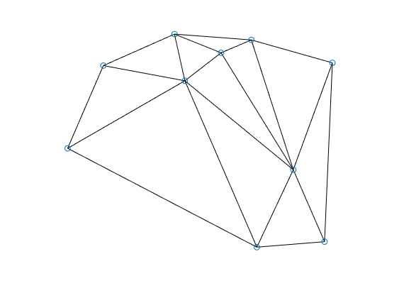
Triangulation of a rectangular mesh
[x,y] = meshgrid(1:10,1:8);
t = delaunay(x(:),y(:));
G = triangleGrid([x(:) y(:)],t);
plot(x(:),y(:),'o','MarkerSize',8);
plotGrid(G,'FaceColor','none');
axis([.9 10 0.9 8]); axis off;
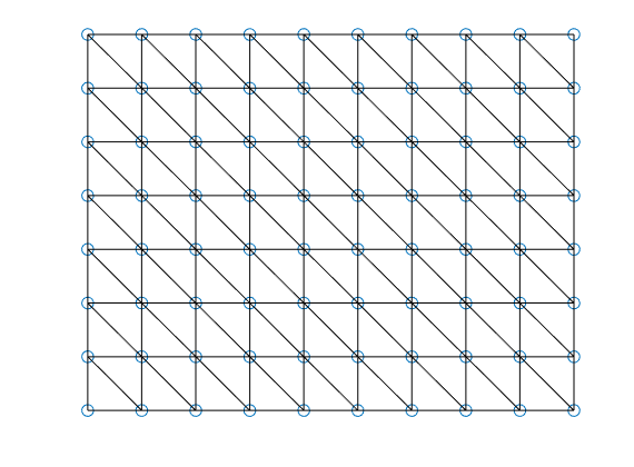
t = delaunayn([x(:) y(:)]);
G = triangleGrid([x(:) y(:)], t);
plot(x(:),y(:),'o','MarkerSize',8);
plotGrid(G,'FaceColor','none');
axis([.9 10 0.9 8]); axis off;
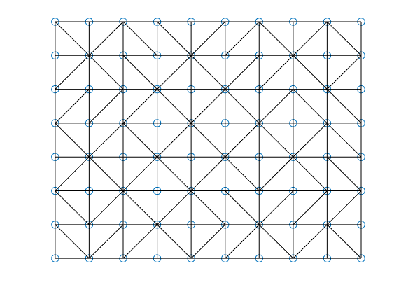
Triangulation of a set of perturbed mesh points
clf;
N=7; M=5; K=3;
[x,y,z] = ndgrid(0:N,0:M,0:K);
x(2:N,2:M,:) = x(2:N,2:M,:) + 0.3*randn(N-1,M-1,K+1);
y(2:N,2:M,:) = y(2:N,2:M,:) + 0.3*randn(N-1,M-1,K+1);
p = [x(:) y(:) z(:)];
t = delaunayn(p);
G = tetrahedralGrid(p,t);
plotGrid(G, 'FaceColor',[.8 .8 .8]); view(-40,60); axis tight off;
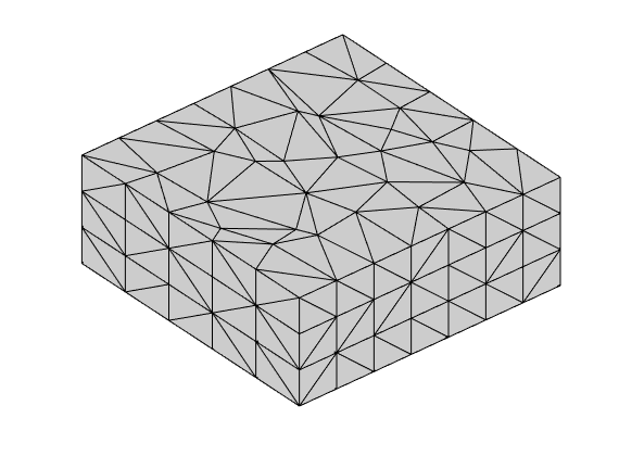
Seamount: A standard example from Matlab
lf
load seamount
t = delaunay(x,y);
G = triangleGrid([x(:) y(:)], t);
plot(x(:),y(:),'o');
plotGrid(G,'FaceColor','none'); axis off
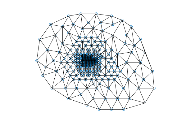
Illustrate the correspondence between Voronoi and Delaunay
Generated from showVoronoiGrids.m
N = 7; M=5;
[x,y]=ndgrid(0:N,0:M);
x(2:N,2:M) = x(2:N,2:M) + 0.3*randn(N-1,M-1);
y(2:N,2:M) = y(2:N,2:M) + 0.2*randn(N-1,M-1);
%
subplot(2,2,1);
plot(x,y,'ok');
axis equal tight off;
%
subplot(2,2,2);
t = delaunay(x,y);
triplot(t,x,y);
hold on; plot(x,y,'ok'); hold off;
axis equal tight off;
%
subplot(2,2,3);
voronoi(x,y);
axis equal tight off;
p=get(gca,'position'); p(2)=p(2)+0.1; set(gca,'position',p);
%
subplot(2,2,4);
h = voronoi(x,y,'b'); set(h,'LineWidth',1);
hold on; triplot(t,x,y,'r','LineWidth',0.25); hold off;
axis equal tight off;
p=get(gca,'position'); p(2)=p(2)+0.1; set(gca,'position',p);
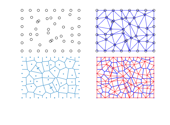
Examples of Voronoi grids
clf;
%
% Regular grid
[x,y] = meshgrid(0:10,0:8);
voronoi(x,y);
axis([1 8 1 5]); axis equal off;
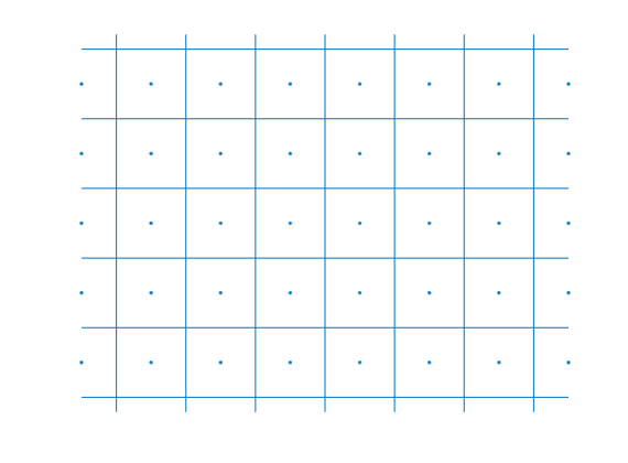
Regular grid
[x,y] = meshgrid(0:10,0:8);
x = [x(:); x(:)+0.5];
y = [y(:); y(:)+0.5];
voronoi(x,y);
axis([1 8 1 5]); axis equal off;
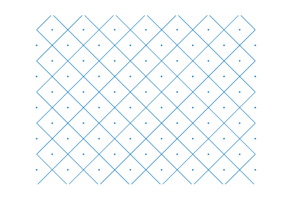
Honeycomb grids
[x,y] = meshgrid((0:10)*2*cos(pi/6),0:8);
x = [x(:); x(:)+cos(pi/6)];
y = [y(:); y(:)+sin(pi/6)];
voronoi(x,y);
axis([1 8 1 5]); axis equal off;
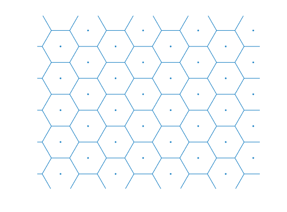
Triangulation of a set of perturbed mesh points
clf;
N=7; M=5;
[x,y] = ndgrid(0:N,0:M);
x(2:N,2:M) = x(2:N,2:M) + 0.3*randn(N-1,M-1);
y(2:N,2:M) = y(2:N,2:M) + 0.3*randn(N-1,M-1);
p = [x(:) y(:)];
T = triangleGrid(p,delaunayn(p));
V = makeLayeredGrid(pebi(T), 3);
plotGrid(V, 'FaceColor',[.8 .8 .8]); view(-40,60); axis tight off;
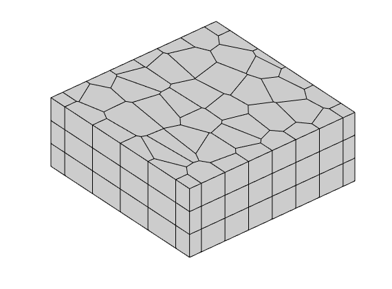
Seamount: A standard example from Matlab
clf
load seamount
V = pebi( triangleGrid([x(:) y(:)], delaunay(x,y)));
plotGrid(V,'FaceColor','none'); axis off;
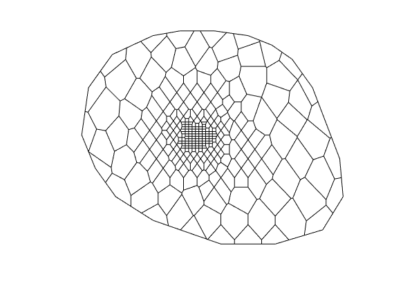
A honeycombed grid
lf
[x,y] = meshgrid((0:4)*2*cos(pi/6),0:3);
x = [x(:); x(:)+cos(pi/6)];
y = [y(:); y(:)+sin(pi/6)];
G = triangleGrid([x(:),y(:)],delaunay(x(:),y(:)));
plotGrid(pebi(G), 'FaceColor','none'); axis equal off
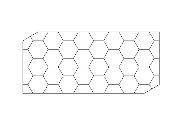
Classic test case: 1D Buckley-Leverett
Generated from buckleyLeverett1D.m
We investigate the effect of time step on the accuracy and convergence of the implicit transport solver
mrstModule add incomp
G = computeGeometry(cartGrid([100,1]));
rock = makeRock(G, 100*milli*darcy, 0.2);
fluid = initSimpleFluid('mu' , [ 1, 1] .* centi*poise , ...
'rho', [1000, 1000] .* kilogram/meter^3, ...
'n' , [ 2, 2]);
bc = fluxside([], G, 'Left', 1, 'sat', [1 0]);
bc = fluxside(bc, G, 'Right', -1, 'sat', [0 1]);
hT = computeTrans(G, rock);
rSol = initState(G, [], 0, [0 1]);
rSol = incompTPFA(rSol, G, hT, fluid, 'bc', bc);
% Explicit tranport solver
rSole = explicitTransport(rSol, G, 10, rock, fluid, 'bc', bc, 'verbose', true);
% Implicit transport solver: try with one time step
[rSoli, report] = ...
implicitTransport(rSol, G, 10, rock, fluid, 'bc', bc, 'Verbose', true);
explicitTransport: Computing transport step in 199 substeps
implicitTransport:
----------------------------------------------------------------------
Time interval (s) iter relax residual rate
----------------------------------------------------------------------
[0.0e+00, 1.0e+01]: 1 1.00 7.82670e+00 NaN
[0.0e+00, 1.0e+01]: 2 0.12 6.81721e+00 0.07
...
Load and display convergence history
Here we have cheated a little: That is, we have copied the screendump to a file and used a text editor to manipulate it so that it can easily be reloaded
figure;
d = load('screendump.dat');
i = isnan(d(:,1)); d(:,1) = 1; d(i,1)=0; d(:,1)=cumsum(d(:,1));
plot(d(:,3),d(:,1),'o-','MarkerFaceColor',[0.5,0.5,0.5]);
set(gca,'XScale','log','YDir','reverse','XDir','normal'); axis tight
set(gca,'XTick',[1e-10 1e-5 1],'FontSize',12);
hold on;
j = find(i);
hold on
plot(repmat([8e-11 10],numel(j),1)',[d(j,1)+.5 d(j,1)+.5]','--r');
hold off
set(gcf,'Position',[1120 55 230 760],'PaperPositionMode','auto');
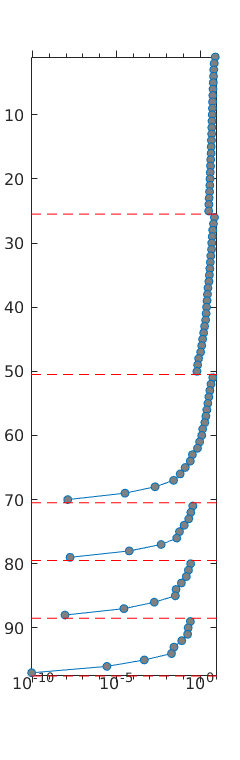
Plot results with various number of time steps
figure
plot(G.cells.centroids(:,1), rSole.s(:,1),'k--','LineWidth',1.5);
leg = cell(7,1); leg{1} = 'Expl: 199 steps';
n = [4 10 20 40 100 200];
its = [0 0 0 0 0 0 0];
col = 'rgbcmk';
hold on
for k=1:numel(n)
rSolt = rSol;
for i=1:n(k)
[rSolt, report] = ...
implicitTransport(rSolt, G, 10/n(k), rock, fluid, 'bc', bc);
its(k) = its(k) + report.iterations + report.vasted_iterations;
end
plot(G.cells.centroids(:,1),rSolt.s(:,1), [col(k) '-'],'LineWidth',1.5);
leg{k+1} = sprintf('n=%3d: %3d its',n(k),its(k));
end
hold off
legend(leg{:});
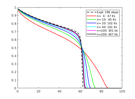
Two-Phase Flow in Inclined Gravity Column
Generated from buoyancyExample.m
In this example, we simulate the injection of a light fluid (CO2) into a heavier fluid (brine) inside an inclined sandbox.
mrstModule add incomp
Set up model
To get an inclined reservoir, we manipulate the gravity direction. Since gravity is a persistent and global variable, it is important that we reset the gravity at the end of the script
theta = 40;
height = 40;
exmpl = 2;
n = [ 20, 2, 100];
box_sz = [100, 10, 200];
% Grid
G = cartGrid(n, box_sz);
G = computeGeometry(G);
CG = cartGrid([1 1 1],box_sz); % used to create outline of sandbox
% Petrophysical data
if exmpl == 1
rock = makeRock(G, 0.1*darcy, 0.3);
else
load rndseed.mat; rng(S);
b = log(milli*darcy);
a = (log(darcy)-b)/(.4 - .05);
p = gaussianField(G.cartDims, [0.05 0.4], [3 1 11], 4.5);
K = exp(a*(p-.05)+b);
rock = makeRock(G, K(:), p(:));
end
T = computeTrans(G, rock, 'verbose', true);
% Fluid
fluid = initSimpleFluid('mu' , [ 0.307, 0.049] .* centi*poise , ...
'rho', [973 , 617 ] .* kilogram/meter^3, ...
'n' , [ 2 , 2 ]);
% Redefine gravity direction
R = makehgtform('yrotate',-pi*theta/180);
gravity reset on
gravity( R(1:3,1:3)*gravity().' );
% Create special colormap
s = linspace(0, 1, 64).';
cm = [1-s.^(13/16), 1-s.^6, s.^6];
Computing one-sided transmissibilities... Elapsed time is 0.004786 seconds.
Set initial data and compute pressure distribution
Put region of CO2 at bottom of reservoir.
xr = initResSol(G, 1*barsa, 1);
d = gravity() ./ norm(gravity);
dc = G.cells.centroids * d.';
xr.s(dc>max(dc)-height) = 0;
xr = incompTPFA(xr, G, T, fluid);
Plot initial data
clf
h = plotGrid(CG, 'FaceColor', 'none', 'EdgeColor', 'k','LineWidth',2);
rotate(h,[0 1 0],theta);
view([0,0])
hs = plotCellData(G, xr.s, xr.s < .995, 'EdgeColor', 'none');
rotate(hs,[0 1 0],theta);
caxis([0 1]); colormap(cm), axis equal tight off
% dPlot = [20 100 250 500 1000 1500 2500 inf]*day;
% print('-dpng', '-r0', sprintf('buoy-%d-%02d.png',exmpl, 0));
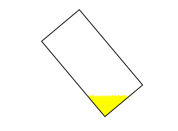
Run simulation
For accuracy, the time step is gradually ramped up
dT = [.5, .5, 1, 1, 1, 2, 2, 2, 5, 5, 10, 10, 15, 20, repmat(25,[1,97])].*day;
[t, ip] = deal(0,1);
for k = 1 : numel(dT)
xr = implicitTransport(xr, G, dT(k), rock, fluid, 'Verbose', false);
% Check for inconsistent saturations
assert (max(xr.s) < 1+eps && min(xr.s) > -eps);
% Increase time and plot saturation
t = t + dT(k);
delete(hs)
hs = plotCellData(G, xr.s, xr.s <.995, 'EdgeColor', 'none');
rotate(hs,[0 1 0],theta);
title(sprintf('%.2f days', t/day));
drawnow
%{
if t>=dPlot(ip)-eps,
colorbar off; title([]);
drawnow;
print('-dpng', '-r0', sprintf('buoy-%d-%02d.png',exmpl, ip));
colorbar, title(sprintf('%.2f days', t/day));
ip = ip+1;
end
%}
% Compute new flow field.
xr = incompTPFA(xr, G, T, fluid);
end
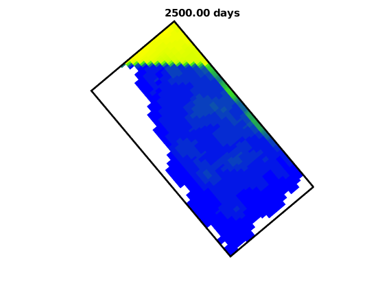
NB: RESET GRAVITY
Gravity is defined as a persistent and global variable and we therefore need to reset it to avoid messing with other examples
gravity reset on
Capillary Equilibrium within Vertical Columns
Generated from capillaryColumn.m
We watch a sharp interface form into a capillary fringe in the vertical direction
mrstModule add incomp
Grid, permeability, and fluid object
gravity reset on
exmpl = 1;
G = computeGeometry(cartGrid([20, 1, 40], [100 1 100]));
if exmpl==1
perm = @(x) (350*x/100 + 50).*milli*darcy;
rock = makeRock(G, perm(G.cells.centroids(:,1)), .1);
dT = .01;
histb = false;
else
load rndseed.mat; rng(S);
b = log(milli*darcy);
a = (log(darcy)-b)/(.4 - .05);
p = gaussianField(G.cartDims, [0.05 0.4], [3 1 11], 4.5);
K = exp(a*(p-.05)+b);
rock = makeRock(G, K(:), p(:));
dT = .1;
histb = true;
end
hT = computeTrans(G, rock);
fluid = initSimpleFluidJfunc('mu' , [0.30860, 0.056641]*centi*poise, ...
'rho', [ 975.86, 686.54]*kilogram/meter^3, ...
'n' , [ 2, 2], ...
'surf_tension',1*barsa/sqrt(mean(rock.poro)/(mean(rock.perm))),...
'rock',rock);
Initial data
t = 0;
xr = initResSol(G, 100.0*barsa, 0.0);
xr.s(G.cells.centroids(:,3)>50) = 1.0;
Plot permeability and prepare for saturation
clf, set(gcf,'Position',[0 450 1280 370]);
cax1 = subplot(1,3,1);
colormap(cax1, parula);
if exmpl==2
plotCellData(G,log10(rock.perm),'EdgeColor','none'); view(0,0), axis tight
[h,az] = colorbarHist(log10(rock.perm),[-14 -12],'South');
set(h,'XTick',-14:-12,'XTickLabel',{'10', '100', '1000'});
else
K = convertTo(rock.perm,milli*darcy);
plotCellData(G,K,'EdgeColor','none'); view(0,0), axis tight
[h,az] = colorbarHist(K,[50 400],'South',40);
end
set(az,'Position',get(az,'Position')-[0 0 0 .02]);
cax2 = subplot(1,3,2);
colormap(cax2, [zeros(128,1) linspace(.8,0,128)' linspace(0,.7,128)']);
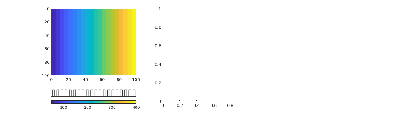
Time loop
dt = dT*[1 1 2 2 3 3 4 4 repmat(5,[1,96])]*year;
dt = [dt(1).*sort(repmat(2.^-[1:5 5],1,1)) dt(2:end)];
s = xr.s(:,1);
for k = 1 : numel(dt)
xr = incompTPFA(xr, G, hT, fluid);
xr = implicitTransport(xr, G, dt(k), rock, fluid);
t = t+dt(k);
% Plot solution
cla
plotCellData(G,xr.s(:,1),'EdgeColor','none');
view(0,0); axis tight; caxis([0 1]);
title(sprintf('time: %.1f yrs', t/year));
drawnow
ds = norm(s - xr.s(:,1),inf);
if ds<1e-4, break, end
fprintf('%e\n',ds);
s = xr.s(:,1);
end
2.621472e-01
1.036592e-01
8.716126e-02
1.040406e-01
1.202392e-01
1.399498e-01
1.539844e-01
1.686116e-01
...
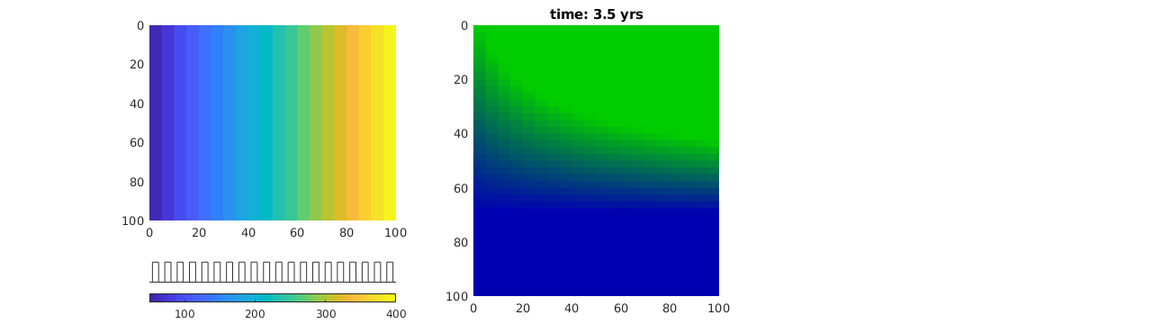
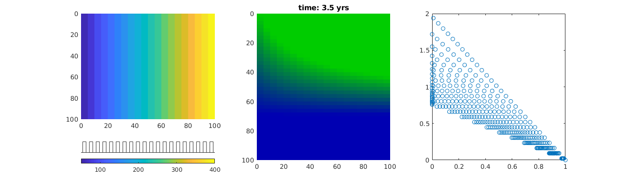
Simulate model with water coning
Generated from coningExample.m
mrstModule add incomp coarsegrid ad-core
Make grid and assign petrophysical properties
G = cartGrid([60,40,10],[1500 1000 200]);
G.nodes.coords(:,3) = G.nodes.coords(:,3)+2050;
G = computeGeometry(G);
[x0,x1,z0,z1] = deal(675,1250,2050,2250);
flt = @(c) (c(:,1)-x0)*(z1-z0)/(x1-x0) + z0 - c(:,3);
rock = makeRock(G, 500*milli*darcy, .2);
rock.perm(flt(G.cells.centroids)>0) = 50*milli*darcy;
rock.poro(flt(G.cells.centroids)>0) = 0.1;
hT = computeTrans(G,rock);
pargs = {'EdgeAlpha',.1,'EdgeColor','k'};
clf, hs = plotCellData(G,rock.perm,pargs{:});
view(3), axis tight
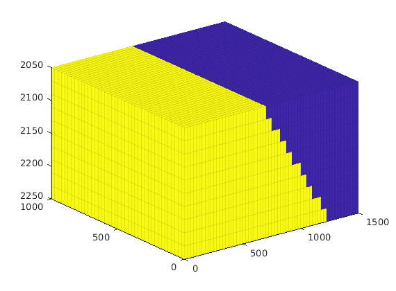
Setup wells
x = G.cells.centroids(:,[1 3]);
W = addWell([], G, rock, find(sum(bsxfun(@minus,x,[67.5 2060]).^2,2)<320), ...
'InnerProduct', 'ip_tpf', ...
'Type', 'bhp', 'Val', 100*barsa, ...
'Comp_i', [0 1], 'Name', 'P', 'Dir','y');
x = G.cells.centroids(:,1:2);
W = addWell(W, G, rock, find(sum(bsxfun(@minus,x,[1437.5 487.5]).^2,2)<320), ...
'InnerProduct', 'ip_tpf',...
'Type', 'bhp', 'Val', 700*barsa, ...
'Comp_i', [1 0], 'Name', 'I', 'Dir','z');
plotWell(G,W,'height',50,'radius',.01);
CG = generateCoarseGrid(G,(flt(G.cells.centroids)>0)+1);
plotFaces(CG,1:CG.faces.num,'FaceColor','none','LineWidth',1);
plotFaces(CG,11,'FaceColor','y','FaceAlpha',.3);
set(hs,'FaceAlpha',.35);
% zoom(1.4);
set(gca,'dataasp',[2 2 1]); view(25,30);
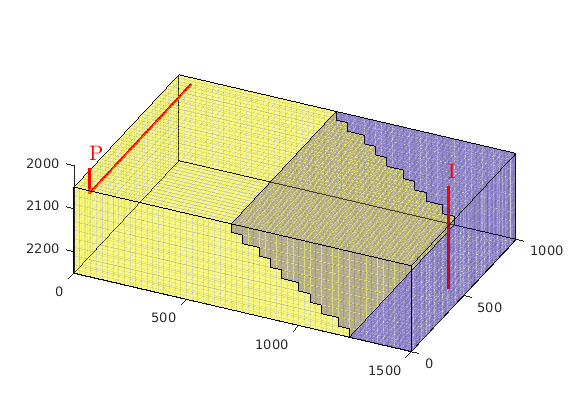
Fluid model
fluid = initSimpleFluid('mu' , [ 1, 10] .* centi*poise , ...
'rho', [1000, 100] .* kilogram/meter^3, ...
'n' , [ 2, 2]);
Simulation loop
N = 450;
T = 4500*day();
dT = T/N*ones(N,1);
dT = [dT(1)*sort(2.^-[1:4 4])'; dT(2:end)];
gravity reset on
rSol = initState(G, W, 0, [0, 1]);
rSol = incompTPFA(rSol, G, hT, fluid, 'wells', W);
t = 0;
pv = poreVolume(G, rock);
oip = sum(rSol.s(:,2).*pv);
colormap(flipud(winter))
wellSols = cell(numel(dT),1);
set(gca,'XTick',[],'Ytick',[],'ZTick',[]);
%
for i=1:numel(dT)
rSol = implicitTransport(rSol, G, dT(i), rock, fluid, 'wells', W);
% Check for inconsistent saturations
assert(max(rSol.s(:,1)) < 1+eps && min(rSol.s(:,1)) > -eps);
% Update solution of pressure equation.
rSol = incompTPFA(rSol , G, hT, fluid, 'wells', W);
% Measure water saturation in production cells in saturation
wellSols{i} = getWellSol(W, rSol, fluid);
% Increase time
t = t + dT(i);
% Plot saturation
delete(hs);
hs = plotCellData(G, rSol.s(:,1), (rSol.s(:,1)>.01), pargs{:});
title([num2str(convertTo(t,day)), ' days']),
caxis([0 1]); drawnow
end
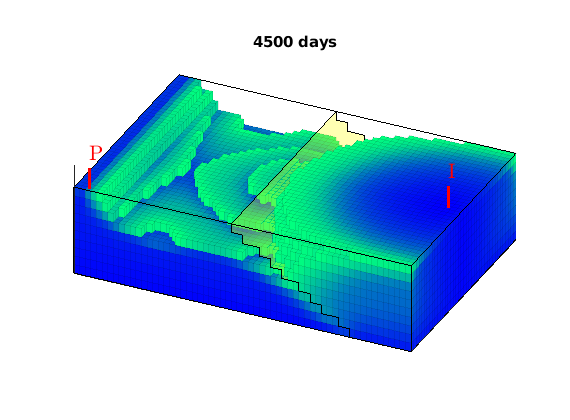
Oil rate, with peak production indicated by red line
figure,
[Ym,Tm] = meshgrid(G.cells.centroids(W(1).cells,2),cumsum(dT)/year);
p = cellfun(@(x) abs(x(1).qO)', wellSols,'UniformOutput',false);
p = vertcat(p{:})*day;
[~,j] = max(p);
m = sub2ind(size(p),j,1:numel(W(1).cells));
surf(Ym,Tm,p); shading interp; colormap(parula(20));
hold on; plot3(Ym(m),Tm(m),p(m), '-r','LineWidth',2); hold off
axis tight, view(100,35)
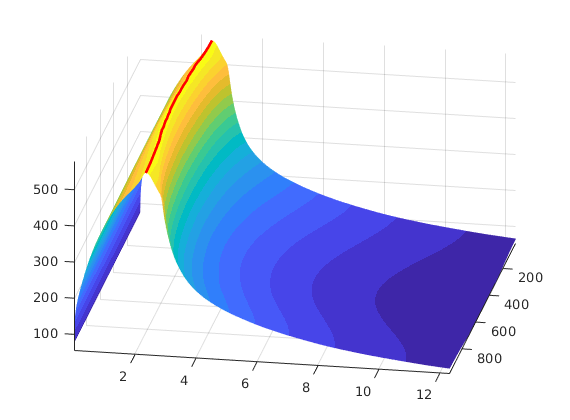
Water production, with breakthrough indicated by red line
figure,
p = cellfun(@(x) abs(x(1).qW)', wellSols,'UniformOutput',false);
p = vertcat(p{:})*day;
j = sum(~(p>1e-3));
m = sub2ind(size(p),j,1:numel(W(1).cells));
surf(Ym,Tm,p); shading interp; colormap(parula(20));
hold on; plot3(Ym(m),Tm(m),p(m), '-r','LineWidth',2); hold off
axis tight, view(45,35)
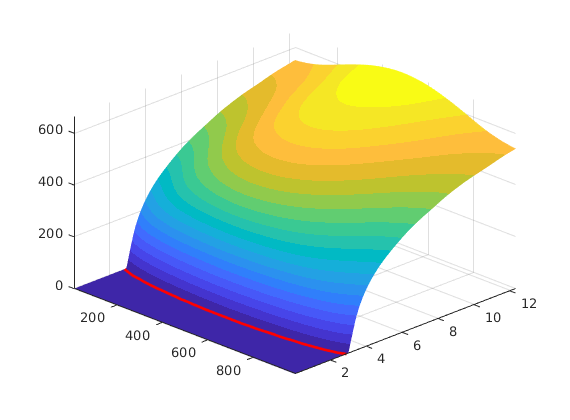
Plot surface rates etc using GUI
plotWellSols(wellSols, cumsum(dT));
%{
%% Oil surface rate
t = cumsum(dT)/day;
qOs = cellfun(@(x) abs(x(1).qOs), wellSols);
figure, set(gca,'Fontsize',24)
plot(t, qOs,'LineWidth',2);
xlabel('Time [days]'); title('Oil surface rate [m^3/s]');
axis tight
%%
figure, set(gca,'Fontsize',24)
plot(t,cumsum(qOs.*dT),'LineWidth',2);
hold on, plot(t([1 end]),[oip oip],'--r','LineWidth',2); hold off
xlabel('Time [days]'); title('Cumulative oil production [m^3]');
axis tight
%% Water surface rate
qWs(:,1) = cellfun(@(x) abs(x(1).qWs), wellSols);
qWs(:,2) = cellfun(@(x) abs(x(2).qWs), wellSols);
figure, set(gca,'Fontsize',24)
plot(t, qWs,'LineWidth',2);
xlabel('Time [days]'); title('Water surface rate [m^3/s]');
axis tight
%%
figure, set(gca,'Fontsize',24)
plot(t,[cumsum(qWs(:,1).*dT) cumsum(qWs(:,2).*dT)],'LineWidth',2);
hold on, plot(t([1 end]),[oip oip],'--r','LineWidth',2); hold off
xlabel('Time [days]'); title('Cumulative oil production [m^3]');
set(gca,'XLim',t([1 end]));
%}
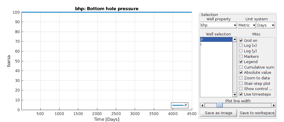
Grid-orientation effects for the five-spot
Generated from gridOrientationQ5.m
With a two-point type discretization (and with many other discretizations as well), evolving displacement profiles will preferrentially move along the axial directions, i.e., in the direction of the normals to the cell faces. To illustrate this, we contrast approximate solutions for the repeated five-spot well pattern computed using the original quarter five-spot setup and with a rotated setup with injectors in the SW and NE corners and producers in the SE and NW corners. The two setups will have different preferrential flow directions and hence generally give different solutions.
mrstModule add incomp
Difference in grid-orientation effects with mobility ratio
This effect is typically associated with instable displacements. To show this we consider three different fluid models with unfavorable mobility ratio, equal viscosities, and favorable mobility ratio.
mu = [1 10; 1 1; 10 1];
pvi = [0.3 0.6 0.7];
cartDim = [32 32 1];
nstep = 16;
set(gcf,'Position',[250 450 1100 360]);
for n=1:3
fluid = initSimpleFluid('mu', mu(n,:).*centi*poise, ...
'rho', [1000, 850].* kilogram/meter^3, 'n', [2, 2]);
subplot(1,3,n)
runQ5DiagParal(cartDim, nstep, fluid, pvi(n));
set(gca,'XTick',[],'YTick',[]);
title(sprintf('Mobility ratio %d:%d. Time: %.1f PVI',...
mu(n,1),mu(n,2),pvi(n)),'FontSize',12); drawnow
end
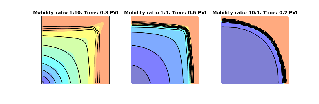
Convergence with respect to time step
m = 1;
fluid = initSimpleFluid('mu', mu(m,:).*centi*poise, ...
'rho', [1000, 850].* kilogram/meter^3, 'n', [2, 2]);
nsteps = [1 8 64];
for n=1:3
subplot(1,3,n)
runQ5DiagParal(cartDim, nsteps(n), fluid, pvi(m));
set(gca,'XTick',[],'YTick',[]);
title(sprintf('Grid: %d x %d. Steps: %d', ...
cartDim(1:2), nsteps(n)),'FontSize',12); drawnow
end
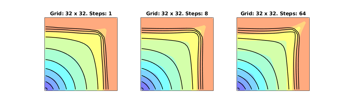
Convergence with respect to spatial resolution
m = 1;
fluid = initSimpleFluid('mu', mu(m,:).*centi*poise, ...
'rho', [1000, 850].* kilogram/meter^3, 'n', [2, 2]);
cartDims = [16 16 1; 32 32 1; 64 64 1];
for n=1:3
subplot(1,3,n)
runQ5DiagParal(cartDims(n,:), nstep, fluid, pvi(m));
set(gca,'XTick',[],'YTick',[]);
title(sprintf('Grid: %d x %d. Steps: %d', ...
cartDims(n,1:2), nstep),'FontSize',12); drawnow
end
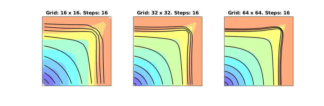
Inverted Gravity Column
Generated from invertedGravityColumn.m
We consider a setup with a heavier fluid placed on top of a lighter fluid. The lighter fluid will move upward and the heavier fluid will move downward and gradually we will approach a stable steady state.
mrstModule add incomp
Define the model
gravity reset on
G = computeGeometry(cartGrid([1, 1, 40], [1, 1, 10]));
rock = makeRock(G, 0.1*darcy, 1);
fluid = initCoreyFluid('mu' , [0.30860, 0.056641]*centi*poise , ...
'rho', [ 975.86, 686.54]*kilogram/meter^3, ...
'n' , [ 2, 2],...
'sr', [ .1, .2],...
'kwm',[ .2142, .85]);
Initialize problem
Set up the fluid distribution, compute pressure
hT = computeTrans(G, rock);
xr = initResSol(G, 100.0*barsa, 1.0); xr.s(end/2+1:end) = 0.0;
xr = incompTPFA(xr, G, hT, fluid); x0 = xr;
% Plot the 3D solution
figure(1);
subplot(1,3,1:2);
plotCellData(G,xr.s(:,1),'EdgeColor','none');
set(gca,'XTick',[],'YTick',[],'Ztick',[]); box on; view(3); caxis([0 1]);
title(sprintf('Time: %.2f years', 0));
colormap(flipud(parula));
% Plot 2D profile of the solution
subplot(1,3,3);
plot(xr.s(:,1),G.cells.centroids(:,3),'-o',...
'MarkerSize',8,'MarkerFaceColor',[.5,.5,.5]);
set(gca,'XTick',[],'YTick',[],'YDir','reverse');
%n=0; print('-depsc2',['inv-column-' num2str(n) '.eps']);
figure(2);
col = jet(16); k=1;
plot(G.cells.centroids(:,3), xr.pressure,'-o','MarkerSize',2,'color',col(k,:),'LineWidth',1.5);
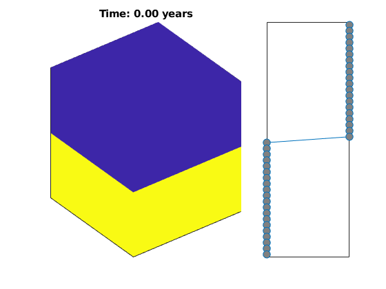
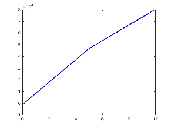
Solve the problem
We use a number of time steps to march the solution towards steady state. Since we do not have any movement in the lateral directions, we can use the explicit solver as a pure gravity segregation solver.
dt = 5*day; t=0;
S = zeros(G.cells.num,151); S(:,1) = xr.s(:,1);
for i=1:150
% Saturation step
xr = explicitTransport(xr, G, dt, rock, fluid, 'onlygrav', true);
t = t+dt;
% Plot 3D solution
figure(1);
subplot(1,3,1:2); cla
plotCellData(G,xr.s(:,1),'EdgeColor','none'), box on; view(3);
set(gca,'XTick',[],'YTick',[],'Ztick',[]); caxis([0 1]);
title(sprintf('Time: %.2f years', t/year));
% Plot 2D profile of the saturation
subplot(1,3,3);
plot(xr.s(:,1),G.cells.centroids(:,3),'-o',...
'MarkerSize',8,'MarkerFaceColor',[.5,.5,.5]);
set(gca,'XTick',[],'YTick',[],'YDir','reverse');
drawnow; pause(0.1);
%if any(i==[25 50 75 100 150])
% n=n+1; print('-depsc2',['inv-column-' num2str(n) '.eps']);
%end
if ~mod(i,10)
k = k+1;
figure(2); hold on;
plot(G.cells.centroids(:,3), xr.pressure,'-','Color',col(k,:),'LineWidth',1.5);
hold off
end
% Compute pressure for the next step
xr = incompTPFA(xr, G, hT, fluid);
S(:,i+1)=xr.s(:,1);
end
figure(2);
hold on
plot(G.cells.centroids(:,3), xr.pressure,'+','Color',col(k,:),'MarkerSize',6);
hold off
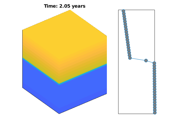
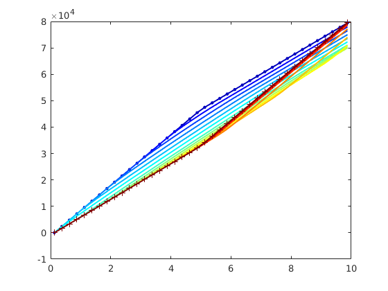
figure;
pcolor(S'); shading interp;
colormap(flipud(parula));
set(gca,'YDir','reverse');
box on; %set(gca,'XTick',[],'YTick',[]);
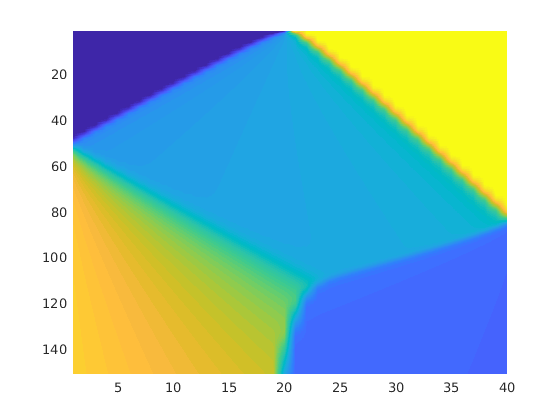
Simulate model with gravity override
Generated from overrideExample.m
We consider a model consisting of two zones of different permeability. A light fluid of high mobility is injected into the lower zone by a vertical well placed near the east side. Fluids are produced from a well placed near the west side and perforated in the lower zone only.
mrstModule add incomp coarsegrid ad-core
Make grid and assign petrophysical properties
The grid has two zones with different permeabilities: high permeability on top and low below, or opposite if inequality sign is reversed in the definition of layer function
G = cartGrid([60,40,10],[1500 1000 200]);
G.nodes.coords(:,3) = G.nodes.coords(:,3)+2050;
G = computeGeometry(G);
[K1,K2,p1,p2] = deal(200,1000,.1,.3);
layer = @(c) (c(:,3)-2150)<0; % <0: high perm on top, >0: low on top
rock = makeRock(G, K1*milli*darcy, p1);
rock.poro(layer(G.cells.centroids)) = p2;
rock.perm(layer(G.cells.centroids)) = K2*milli*darcy;
hT = computeTrans(G,rock);
clf
pargs = {'EdgeAlpha',.1,'EdgeColor','k'};
hs = plotCellData(G,rock.perm,pargs{:});
view(3), axis tight
set(hs,'FaceAlpha',.35);
% zoom(1.4);
set(gca,'dataasp',[2 2 1]); view(27,-12);
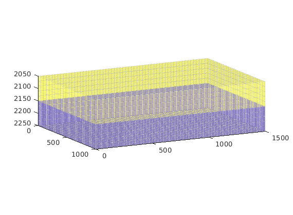
Setup wells
Both wells are perforated in the lower zone only.
T = 1500*day();
x = G.cells.centroids(:,1:2);
W = addWell([], G, rock,...
find( sum(bsxfun(@minus,x,[67.5 487.5]).^2,2)<320 ...
& G.cells.centroids(:,3)>2150), ...
'InnerProduct', 'ip_tpf', ...
'Type', 'bhp', 'Val', 100*barsa, ...
'Comp_i', [0 1], 'Name', 'P', 'Dir','z');
x = G.cells.centroids(:,1:2);
W = addWell(W, G, rock, ...
find( sum(bsxfun(@minus,x,[1437.5 487.5]).^2,2)<320 ...
& G.cells.centroids(:,3)>2150), ...
'InnerProduct', 'ip_tpf',...
'Type', 'rate', 'Val', .8*sum(poreVolume(G,rock))/T, ...
'Comp_i', [1 0], 'Name', 'I', 'Dir','z');
plotWell(G,W,'height',75,'radius',.01);
CG = generateCoarseGrid(G,(layer(G.cells.centroids)>0)+1);
plotFaces(CG,1:CG.faces.num,'FaceColor','none','LineWidth',1);
plotFaces(CG,11,'FaceColor','y','FaceAlpha',.3);
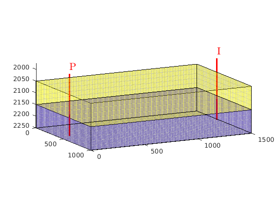
Fluid model
Inject a light and mobilt fluid into a denser and less mobile fluid
fluid = initSimpleFluid('mu' , [ .1, 1] .* centi*poise , ...
'rho', [ 700,1000] .* kilogram/meter^3, ...
'n' , [ 2, 2]);
Simulation loop
N = 100;
dT = T/N*ones(N,1);
dT = [dT(1)*sort(2.^-[1:4 4])'; dT(2:end)];
gravity reset on
rSol = initState(G, W, 0, [0, 1]);
rSol = incompTPFA(rSol, G, hT, fluid, 'wells', W);
t = 0;
colormap(flipud(winter))
wellSols = cell(numel(dT),1);
set(gca,'XTick',[],'Ytick',[],'ZTick',[]);
%
for i=1:numel(dT)
rSol = implicitTransport(rSol, G, dT(i), rock, fluid, 'wells', W);
% Check for inconsistent saturations
assert(max(rSol.s(:,1)) < 1+eps && min(rSol.s(:,1)) > -eps);
% Update solution of pressure equation.
rSol = incompTPFA(rSol , G, hT, fluid, 'wells', W);
% Measure water saturation in production cells in saturation
wellSols{i} = getWellSol(W, rSol, fluid);
% Increase time
t = t + dT(i);
% Plot saturation
delete(hs);
hs = plotCellData(G, rSol.s(:,1), (rSol.s(:,1)>.01), pargs{:});
title([num2str(convertTo(t,day)), ' days']),
caxis([0 1]); drawnow
end
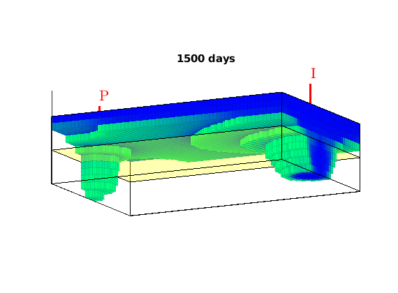
Oil rate, with peak production indicated by red line
figure,
[Ym,Tm] = meshgrid(G.cells.centroids(W(1).cells,3),cumsum(dT)/year);
p = cellfun(@(x) abs(x(1).qO)', wellSols,'UniformOutput',false);
po = vertcat(p{:})*day;
[~,j] = max(po);
m = sub2ind(size(po),j,1:numel(W(1).cells));
surf(Ym,Tm,po); shading interp; colormap(parula(20));
hold on; plot3(Ym(m),Tm(m),po(m), '-r','LineWidth',2); hold off
axis tight, view(100,35)
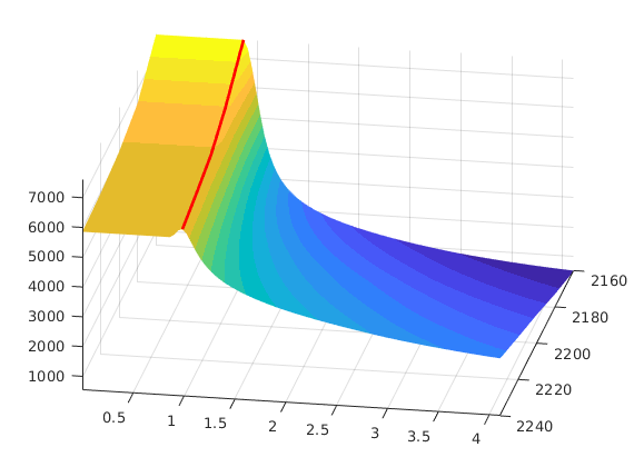
Water production, with breakthrough indicated by red line
figure,
p = cellfun(@(x) abs(x(1).qW)', wellSols,'UniformOutput',false);
pw = vertcat(p{:})*day;
j = sum(~(pw>1e-3));
m = sub2ind(size(pw),j,1:numel(W(1).cells));
surf(Ym,Tm,pw); shading interp; colormap(parula(20));
hold on; plot3(Ym(m),Tm(m),pw(m), '-r','LineWidth',2); hold off
axis tight, view(45,35)
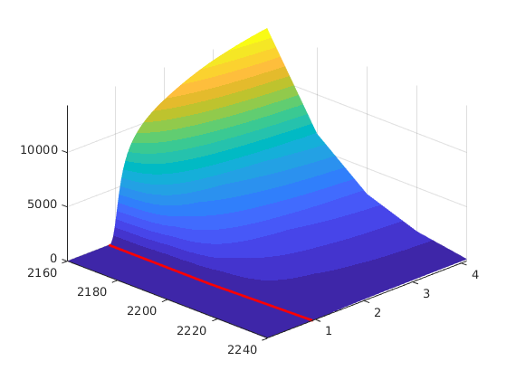
Total rate, with breakthrough indicated by red line
figure,
p = po + pw;
surf(Ym,Tm,p); shading interp; colormap(parula(20));
hold on; plot3(Ym(m),Tm(m),p(m), '-r','LineWidth',2); hold off
axis tight, view(45,35)
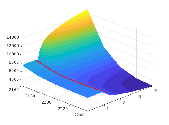

Homogeneous quarter five-spot
Generated from quarterFiveSpot2D.m
In this example, we compare and contrast incompressible single-phase and two-phase flow for a homogeneous quarter five-spot. Through the example, you will also be introduced to the way well solutions are represented in more advanced multiphase simulators based on the AD-OO framework.
mrstModule add incomp diagnostics
Set up model
Square domain with homogeneous rock properties, no flow across the boundaries, no gravity, injection in the southeast and production in the northwest corners, both operating at fixed bottom-hole pressure
gravity reset off
cartDim = [128 128 1];
fluid = initSimpleFluid('mu' , [ 1, 1] .* centi*poise , ...
'rho', [1000, 850] .* kilogram/meter^3, ...
'n' , [ 2, 2]);
domain = [250 250 20];
G = computeGeometry(cartGrid(cartDim,domain));
rock = makeRock(G, 100*milli*darcy, 0.2);
pv = poreVolume(G, rock);
W = addWell([],G, rock, 1, 'Type', 'bhp', ...
'Val', 100*barsa, 'name', 'I', 'radius', .1, 'Comp_i', [1 0]);
W = addWell(W,G, rock, G.cells.num, 'Type', 'bhp', ...
'Val', 0, 'name', 'P', 'radius', .1, 'Comp_i', [0 1]);
hT = computeTrans(G, rock);
% Figure, colormap and contour values
figure('Position',[300 550 1100 650]);
nval = 20;
cval = linspace(0,1,nval+1); cval=.5*cval(1:end-1)+.5*cval(2:end);
colormap(flipud(.5*jet(nval)+.5*ones(nval,3)));

Compute solution and plot saturation evolution
To study the solution, we will plot saturation profiles at four instances in time up to slightly beyond water breakthrough; this corresponds dimensionless times 0.2 to 0.8 PVI. To get the solution provies as accurate as possible, we use the explicit transport solver and M substeps to advance the solution 0.2 PVI forward in time. We continue computing the solution up to time 1.2 PVI, but do not show snapshots of the saturation field for the two last time intervals.
% Compute an initial single-phase pressure solution, from which we estimate
% the final time that corresponds to 1.2 PVI if this flow field remains
% unchanged. With quadratic relperm curves and equal viscosities, the
% multiphase displacement front will propagate at a speed of
% a=1/(2(sqrt(2)-1)) relative to the total velocity.
x = initState(G,W,100*barsa, [0 1]);
x = incompTPFA(x, G, hT, fluid, 'wells', W);
T = 1.2*sum(pv)/x.wellSol(1).flux;
a = 1/(2*(sqrt(2)-1));
% Compute time-of-flight for the single-phase flow field and record the
% corresponding breakthrough time in the producer.
tau = computeTimeOfFlight(x, G, rock, 'wells', W);
tbf = tau(W(2).cells,1);
% Initialize number of time intervals, cell array to hold well solutions,
% and array to hold the oil in place
[N,M] = deal(6,10);
wellSols = cell(N*M+1,1); wellSols{1} = getWellSol(W, x, fluid);
oip = zeros(N*M+1,1); oip(1) = sum(x.s(:,2).*pv);
for n=1:N
fprintf(1,'Main step %d: ',n);
for m=1:M
x = incompTPFA(x, G, hT, fluid, 'wells', W);
x = explicitTransport(x, G, T/(N*M), rock, fluid, 'wells', W);
wellSols{(n-1)*M+m+1} = getWellSol(W, x, fluid);
oip((n-1)*M+m+1) = sum(x.s(:,2).*pv);
if x.s(W(2).cells,1)<eps
W(2).bt = (n-1)*M+m+1;
end
fprintf(1,'%d, ',m);
end
fprintf(1,'\n');
if n>4, continue, end
% Plot multiphase solution
subplot(2,4,n);
contourf(reshape(G.cells.centroids(:,1), G.cartDims),...
reshape(G.cells.centroids(:,2), G.cartDims), ...
reshape(x.s(:,1),G.cartDims), [0 cval 1], 'EdgeColor','none');
hold on;
% Plot corresponding time lines from single-phase solution
contour(reshape(G.cells.centroids(:,1), G.cartDims),...
reshape(G.cells.centroids(:,2), G.cartDims), ...
reshape(tau/T,G.cartDims), a*n/N, '-k','LineWidth',1);
caxis([0 1]);
axis equal; axis([0 domain(1) 0 domain(2)]);
title(sprintf('t=%.2f PVI',n*.2));
set(gca,'XTick',[],'YTick',[]);
% Plot multiphase solution as function of single-phase time-of-flight
subplot(2,4,4+n)
set(gca,'position',get(gca,'position')+[0 .12 0 0]);
plot(tau(:,1)/tbf,x.s(:,1),'.k','MarkerSize',4);
set(gca,'XLim',[0 2]); drawnow;
end
Main step 1: 1, 2, 3, 4, 5, 6, 7, 8, 9, 10,
Main step 2: 1, 2, 3, 4, 5, 6, 7, 8, 9, 10,
Main step 3: 1, 2, 3, 4, 5, 6, 7, 8, 9, 10,
Main step 4: 1, 2, 3, 4, 5, 6, 7, 8, 9, 10,
Main step 5: 1, 2, 3, 4, 5, 6, 7, 8, 9, 10,
Main step 6: 1, 2, 3, 4, 5, 6, 7, 8, 9, 10,
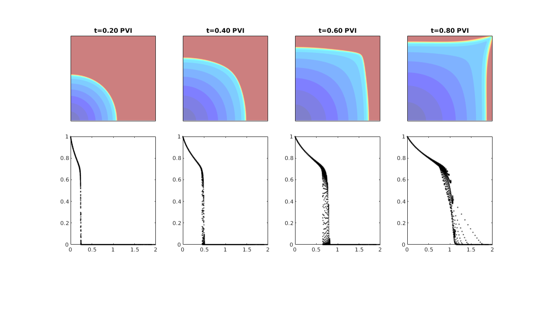
Plot production curves
First we plot the saturation in the perforated cell and the corresponding water cut, i.e., the fractional flow evaluated in the completion
dt = [0; ones(N*M,1)*T/(N*M)]; t = 1.2*cumsum(dt)/T;
figure;
plot(t,cellfun(@(x) x(2).Sw, wellSols),'--', ...
t,cellfun(@(x) x(2).wcut, wellSols),'-','LineWidth',1);
legend('Sw in completion','Water cut','Location','NorthWest');
axis([0 max(t) -.05 1.0]);
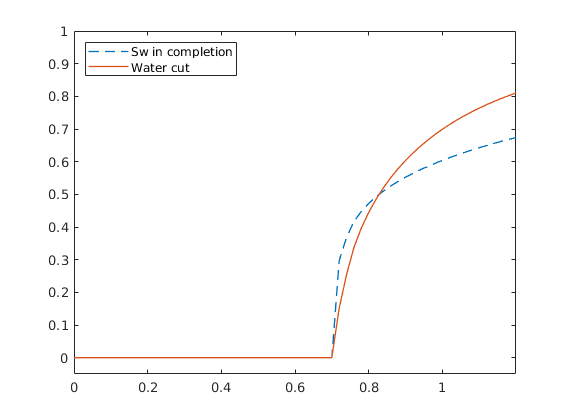
Second, we plot the oil rate used in our simulation in units m^3/day
figure;
qOs = cellfun(@(x) abs(x(2).qOs), wellSols);
stairs(t, qOs([2:end end])*day,'LineWidth',1); axis([0 1.2 30 260]);
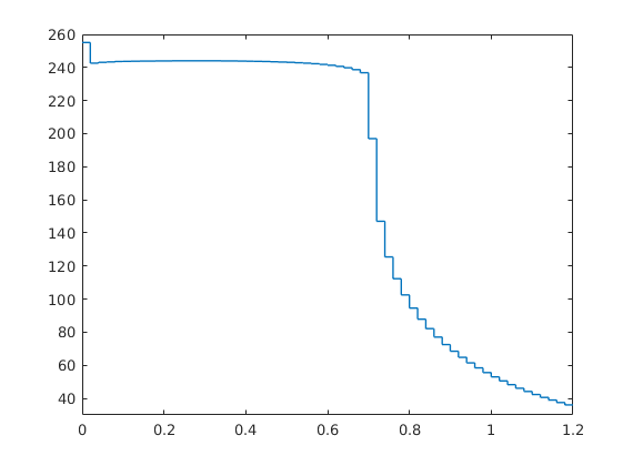
Last, we plot the cumulative oil production computed from the well solution and compare this with the amount of extracted oil derived from a mass-balance computation (initial oil in place minus current oil in place). We also include a horizontal line indicating the initial oil in place, and a straight line showing the amount of oil we would have extracted if oil was produced at the constant initial rate
figure
plot(t,cumsum(bsxfun(@times, abs(cellfun(@(x) x(2).qOs, wellSols)), dt)));
hold on;
plot(t,oip(1)-oip,'-.','LineWidth',3);
plot([0 1.2],oip([1 1]),'-k',t,min(t*oip(1),oip(1)),'-k', ...
t(W(2).bt+[0 0]),[0 oip(1)],'--k');
hold off; axis tight; axis([0 max(t) 0 1.05*oip(1)]);
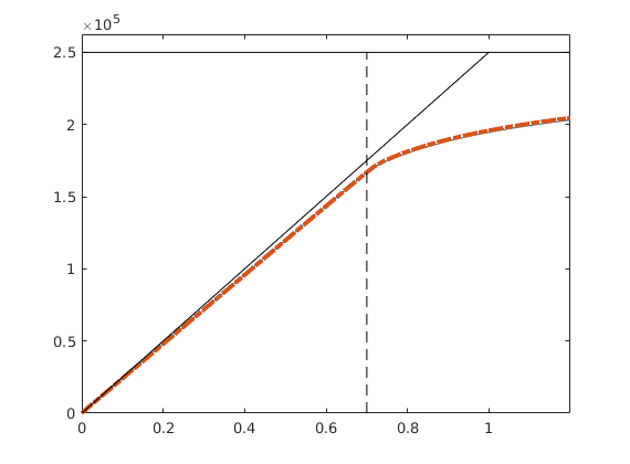
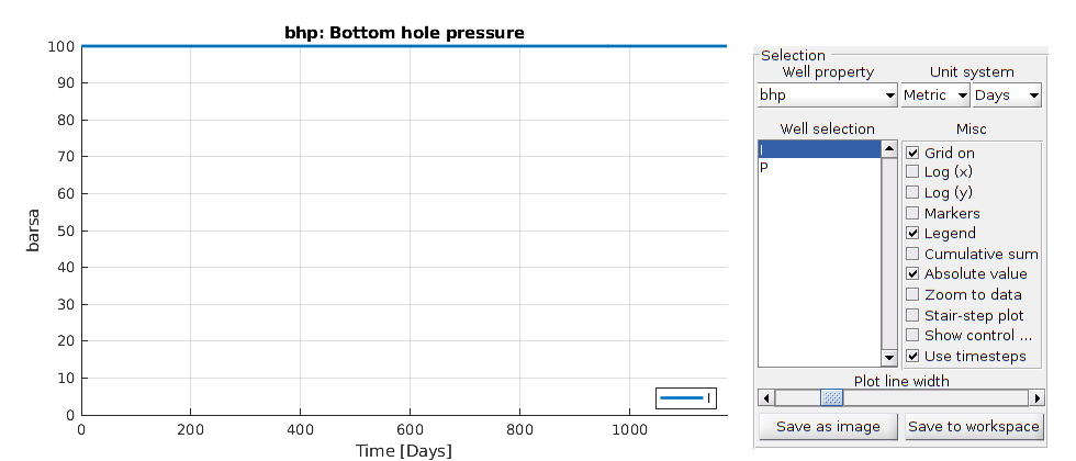
Two-Phase Incompressible Simulation on the Norne Model
Generated from runNorneSynthetic.m
In this example, we will consider the grid and the petrophysical properties from the Norne simulation model to demonstrate some of the complexity one will see in a real simulation model. We set up a two-phase simulation that uses synthetic fluid model, well placement, and simulation schedule. Norne is an oil and gas field lies located in the Norwegian Sea. The reservoir is found in Jurrasic sandstone at a depth of 2500 meter below sea level. Operator Statoil and partners (ENI and Petoro) have agreed with NTNU to release large amounts of subsurface data from the Norne field for research and education purposes. The Norne Benchmark datasets are hosted and supported by the Center for Integrated Operations in the Petroleum Industry (IO Center) at NTNU. Recently, the OPM Initiative released the full simulation model as an open data set on GitHub.
mrstModule add deckformat incomp
gravity reset on
Read and process the model
As the Norne dataset is available from the OPM project’s public GitHub repository, we can download a suitable subset of the simulation model and process that subset. See the showNorne script for a more detailed walkthrough of the model.
if ~ (makeNorneSubsetAvailable() && makeNorneGRDECL())
error('Unable to obtain simulation model subset');
end
grdecl = fullfile(getDatasetPath('norne'), 'NORNE.GRDECL');
grdecl = readGRDECL(grdecl);
grdecl = convertInputUnits(grdecl, getUnitSystem('METRIC'));
Extract the active part of the model
To get the whole grid, we need to reprocess the input data. This gives a grid with two components: the main reservoir and a detached stack of twelve cells, which we ignore henceforth.
G = processGRDECL(grdecl);
G = computeGeometry(G(1));
Set view parameters and plot grid
myview = struct(...
'view', [-110,50], ...
% view angle
'zoom', 1.8, ...
% zoom
'dataasp', [1 1 .1], ...
% data aspect ratio
'dolly', [0 .1 0], ...
% camdolly
'pargs', {{'EdgeAlpha'; 0.1; 'EdgeColor'; 'k'}} ...
);
clf
plotReservoirModel(G, [], [], myview);
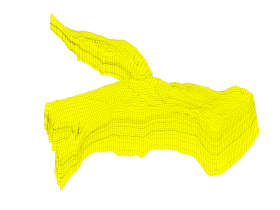
Outline petrophysical properties
The petrophysical properties are included in the simulation model subset represented by function makeNorneSubsetAvailable. Consequently, the necessary data has been read into the grdecl structure. We can then extract the petrophysical properties. Notice that here, the rock
rock = grdecl2Rock(grdecl, G.cells.indexMap);
Porosity and net-to gross
Show the porosities mapped onto the structural grid
figure,
plotReservoirModel(G, rock.poro, [], myview);
colorbarHist(rock.poro, [.05 .35],'South',100);
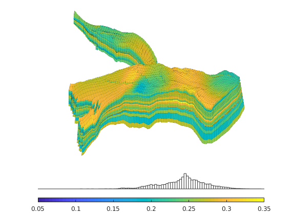
show also the net-to-gross
figure
plotReservoirModel(G, rock.ntg, [], myview);
colorbarHist(rock.ntg,[.07 1],'South',100);
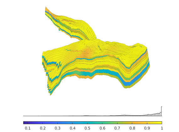
Permeability
The permeability is generally a tridiagonal tensor K = diag(Kx, Ky, Kz). For the Norne model, the data file only specifies Kx, and then various manipulations are done to get the correct vertical permeability.
figure,
prms = myview;
prms.cs = [1 10 100 1000 10000];
prms.unit = milli*darcy;
prms.cb = 'South';
plotReservoirModel(G, log10(rock.perm(:,1)), [], prms);
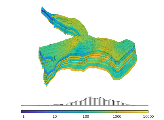
figure,
prms.cs = [0.1 1 10 100 1000 3000];
plotReservoirModel(G, log10(rock.perm(:,3)), [], prms);
%caxis(log10([.1 2500]*milli*darcy));
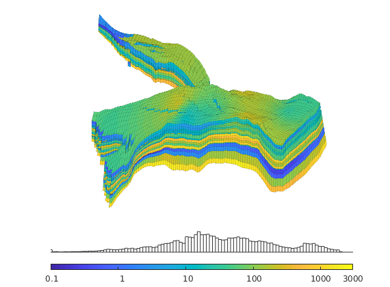
Multipliers
The model has a number of multipliers that reduce the transmissibility in the z-direction
figure
prms = myview;
prms.pargs = {'FaceColor','none','EdgeAlpha',.1,'EdgeColor','k'};
plotReservoirModel(G, [], [], prms);
mz = grdecl.MULTZ(G.cells.indexMap);
plotCellData(G,mz,mz<1,myview.pargs{:});
mz(mz==1) = nan;
colorbarHist(mz, [-.05 .6], 'South', 100);
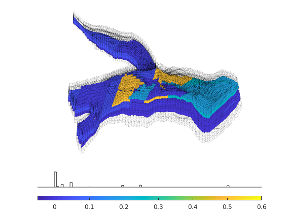
Introduce wells
The reservoir is produced using a set production wells controlled by bottom-hole pressure and rate-controlled injectors. Wells are described using a Peacemann model, giving an extra set of equations that need to be assembled. For simplicity, all wells are assumed to be vertical and are assigned using the logical (i,j) subindex.
% Set vertical injectors, completed in the lowest 12 layers.
nz = G.cartDims(3);
I = [ 9, 26, 8, 25, 35, 10];
J = [14, 14, 35, 35, 68, 75];
R = [ 4, 4, 4, 4, 4, 4]*1000*meter^3/day;
nIW = 1:numel(I); W = [];
for i = 1 : numel(I)
W = verticalWell(W, G, rock, I(i), J(i), nz-11:nz, 'Type', 'rate', ...
'InnerProduct', 'ip_tpf', ...
'Val', R(i), 'Radius', 0.1, 'Comp_i', [1, 0], ...
'name', ['I', int2str(i)], 'refDepth', 2500);
end
% Set vertical producers, completed in the upper 14 layers
I = [17, 12, 25, 35, 15];
J = [23, 51, 51, 95, 94];
P = [300, 300, 300, 200, 200];
nPW = (1:numel(I))+max(nIW);
for i = 1 : numel(I)
W = verticalWell(W, G, rock, I(i), J(i), 1:14, 'Type', 'bhp', ...
'InnerProduct', 'ip_tpf', ...
'Val', 300*barsa(), 'Radius', 0.1, 'refDepth', 2500, ...
'name', ['P', int2str(i)], 'Comp_i', [0, 1]);
end
% Plot grid outline and the wells
figure
myview = struct(...
'view', [30,50], ...
% view angle
'zoom', 1.8, ...
% zoom
'dataasp', [15 15 2], ...
% data aspect ratio
'cb', 'horiz', ...
% colorbar location
'dolly', [0 .3 0], ...
% camdolly
'wargs', {{'height', 30, 'Color', 'k', 'FontSize', 10}}, ...
'pargs', {{'FaceColor', 'none', 'EdgeAlpha', .05}} ...
);
plotReservoirModel(G, [], W, rmfield(myview,'cb'));
plotGrid(G, vertcat(W(nIW).cells), 'FaceColor', 'b');
plotGrid(G, vertcat(W(nPW).cells), 'FaceColor', 'r');
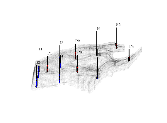
Transmissibilities and initial state
Initialize solution structures and compute transmissibilities from input grid, rock properties, and well structure.
hT = computeTrans(G, rock, 'Verbose', true);
tmult = computeTranMult(G, grdecl);
hT = hT.*tmult;
rSol = initState(G, W, 0, [0, 1]);
Computing one-sided transmissibilities...
Warning:
5512 negative transmissibilities.
Replaced by absolute values...
Elapsed time is 0.039221 seconds.
Fluid model
fluid = initSimpleFluid('mu' , [ 1, 5]*centi*poise , ...
'rho', [1014, 859]*kilogram/meter^3, ...
'n' , [ 2, 2]);
Prepare plotting of saturations
figure
myview.zoom = 2.05; myview.dolly = [0,.2,0];
h = plotReservoirModel(G, [], W, myview);
colormap(flipud(winter))
set(h,'Position',[.13 .07 .77 .05]);
[hs,ha] = deal([]); caxis([0 1]);
drawnow
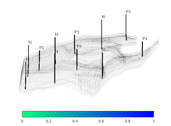
Main loop
In the main loop, we alternate between solving the transport and the flow equations. The transport equation is solved using the standard implicit single-point upwind scheme with a simple Newton-Raphson nonlinear solver.
T = 12*year();
dplt = .25*year;
pv = poreVolume(G,rock);
t = 0; plotNo = 1;
dt = diff(0:year/12:T);
dt = [dt(1).*sort(repmat(2.^-[1:5 5],1,1)) dt(2:end)];
wSol = cell(numel(dt),1);
for n=1:numel(dt)
rSol = incompTPFA(rSol, G, hT, fluid, 'wells', W);
rSol = implicitTransport(rSol, G, dt(n), rock, fluid, 'wells', W);
% Check for inconsistent saturations
assert(max(rSol.s(:,1)) < 1+eps && min(rSol.s(:,1)) > -eps);
% Extract well data
wSol{n} = getWellSol(W, rSol, fluid);
% Increase time and continue if we do not want to plot saturations
t = t + dt(n);
if ( t < plotNo*dplt && t <T), continue, end
% Plot saturation
delete([hs, ha])
hs = plotCellData(G, rSol.s(:,1), find(rSol.s(:,1) > 0.01),'EdgeColor','none');
ha = annotation('textbox', [0 0.93 0.35 0.07], 'String', ...
sprintf('Water saturation at %5.2f years', convertTo(t,year)));
drawnow
plotNo = plotNo+1;
end
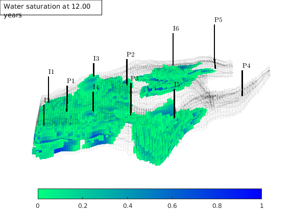
Demonstrate various analytical fluid models
Generated from showFluidObjects.m
mrstModule add incomp
Simple fluid model
fluid = initSimpleFluid('mu' , [ 1, 1]*centi*poise , ...
'rho', [1000, 1000]*kilogram/meter^3, ...
'n' , [ 3, 3]);
s=linspace(0,1,20)';
kr = fluid.relperm(s);
plot(s,kr(:,1),'-s',s,kr(:,2),'-o');
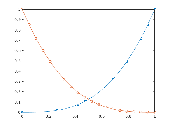
Corey fluid model
fluid = initCoreyFluid('mu' , [ 1, 10]*centi*poise , ...
'rho', [1014, 859]*kilogram/meter^3, ...
'n' , [ 3, 2.5] , ...
'sr' , [ 0.2, 0.15] , ...
'kwm', [ 1, .85]);
s=linspace(0,1,50)';
[kr,dkr,ddkr] = fluid.relperm(s);
subplot(1,3,1),
plot(s(s<.85),kr(s<.85,1),s(s>.2),kr(s>.2,2),'LineWidth',1); axis([0 1 -.02 1]);
subplot(1,3,2),
plot(s(s<.85),dkr(s<.85,1),s(s>.2),dkr(s>.2,4),'LineWidth',1); axis([0 1 -.1 4.5]);
subplot(1,3,3),
plot(s(s<.85),ddkr(s<.85,1),s(s>.2),ddkr(s>.2,2),'LineWidth',1); axis([0 1 -.2 9.5]);
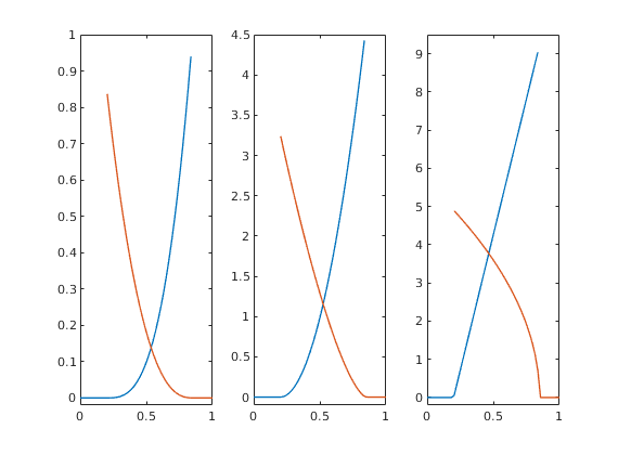
Simple fluid with linear capillary term
fluid = initSimpleFluidPc('mu' , [ 1, 10]*centi*poise , ...
'rho', [1014, 859]*kilogram/meter^3, ...
'n' , [ 2, 2], ...
'pc_scale', 2*barsa);
s = linspace(0, 1, 101).'; kr = fluid.relperm(s);
subplot(1,2,1), plot(s, kr), legend('kr_1(S)', 'kr_2(S)')
x.s = [s 1-s]; pc = fluid.pc(x);
subplot(1,2,2), plot(s, pc); legend('P_c(S)');
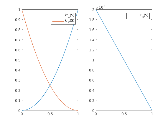
Simple model with Leverett-J function
G = computeGeometry(cartGrid([40,5,1],[1000 500 1]));
state.s = G.cells.centroids(:,1)/1000;
p = G.cells.centroids(:,2)*.001;
rock = makeRock(G, p.^3.*(1e-5)^2./(0.81*72*(1-p).^2), p);
fluid = initSimpleFluidJfunc('mu' , [ 1, 10]*centi*poise , ...
'rho', [1014, 859]*kilogram/meter^3, ...
'n' , [ 2, 2], ...
'surf_tension',10*barsa/sqrt(0.1/(100*milli*darcy)),...
'rock',rock);
plot(state.s, fluid.pc(state)/barsa,'o');
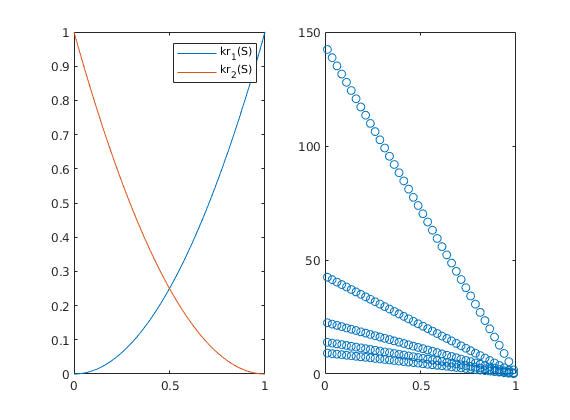
Compare grid-orientation effects for skew grids
Generated from skewGridErrors.m
In this example we consider a symmetric well pattern on a skew grid to study the grid-orientation effects for the combined single-point upwind and TPFA/mimetic schemes. The script contains two different examples, both describing a 400 x 100 m^2 reservoir section. The first (exmpl=1) describes a horizontal reservoir cross-section in which water is injected from one well at the midpoint of the north perimeter and fluids are produced from two wells along the south perimeter, located 50 m from the SE and SW corners, respectively. The second case (exmpl=2) describes a vertical cross-section, where water is injected from two horizontal injectors at the bottom of the reservoir and fluids produced from a horizontal producer at the top of the reservoir. In both cases, the well operate under bottom-hole control.
mrstModule add incomp mimetic ad-core
gravity reset off;
exmpl = 1; % type of cross-section: 1 - horizontal, 2 - vertical
% Final time and number of time steps
T = 1200*day;
nstep =120;
% Rectangular reservoir with a skew grid.
G = cartGrid([41,20],[2,1]);
makeSkew = @(c) c(:,1) + .4*(1-(c(:,1)-1).^2).*(1-c(:,2));
G.nodes.coords(:,1) = 200*makeSkew(G.nodes.coords);
G.nodes.coords(:,2) = 100*G.nodes.coords(:,2);
G = computeGeometry(G);
% Homogeneous reservoir properties
rock = makeRock(G, 100*milli*darcy, .2);
pv = sum(poreVolume(G,rock));
hT = computeTrans(G, rock);
IP = computeMimeticIP(G, rock);
% Symmetric well pattern
wcells = findEnclosingCell(G,[200 97.5; 50 2.5; 350 2.5]);
rate = sum(poreVolume(G,rock));
if exmpl==1
W = addWell([], G, rock, wcells(1), 'Type', 'bhp', ...
'Val', 200*barsa, 'name', 'I', 'radius', .1, 'Comp_i', [1 0]);
W = addWell(W, G, rock, wcells(2), 'Type', 'bhp', ...
'Val', 100*barsa, 'name', 'P1', 'radius', .1, 'Comp_i', [0 1]);
W = addWell(W, G, rock, wcells(3), 'Type', 'bhp', ...
'Val', 100*barsa, 'name', 'P2', 'radius', .1, 'Comp_i', [0 1]);
else
gravity(norm(gravity())*[0 -1 0]);
W = addWell([], G, rock, wcells(1), 'Type', 'bhp', ...
'Val', 100*barsa, 'name', 'P', 'radius', .1, 'Comp_i', [0 1]);
W = addWell(W, G, rock, wcells(2), 'Type', 'bhp', ...
'Val', 200*barsa, 'name', 'I1', 'radius', .1, 'Comp_i', [1 0]);
W = addWell(W, G, rock, wcells(3), 'Type', 'bhp', ...
'Val', 200*barsa, 'name', 'I2', 'radius', .1, 'Comp_i', [1 0]);
end
% Two-phase fluid
fluid = initSimpleFluid('mu', [1 10].*centi*poise, ...
'rho', [1000, 850].* kilogram/meter^3, 'n', [2, 2]);
Prepare plotting and allocate various objects
Figure and figure settings
igure('Position',[400 460 900 350]);
pargs = {'EdgeColor','k','EdgeAlpha',.05};
[xtp,xmi] = deal(initState(G,W,100*barsa, [0 1]));
dt = repmat(T/nstep,1,nstep);
dt = [dt(1).*sort(repmat(2.^-[1:5 5],1,1)) dt(2:end)];
N = numel(dt);
wellSols = cell(N,2);
t = 0;
for n=1:N
t = t + dt(n);
xtp = incompTPFA(xtp, G, hT, fluid, 'wells', W);
xtp = implicitTransport(xtp, G, dt(n), rock, fluid, 'wells', W);
wellSols{n,1} = getWellSol(W, xtp, fluid);
subplot(2,2,1), cla,
plotCellData(G, xtp.pressure/barsa, pargs{:});
caxis([100 200]); title(sprintf('TPFA: %.0f days', t/day));
subplot(2,2,3), cla,
% plotGrid(G,'FaceColor','none');
plotCellData(G, xtp.s(:,1),xtp.s(:,1)>.01,pargs{:});
axis([0 400 0 100]); caxis([0 1]);
xmi = incompMimetic(xmi, G, IP, fluid, 'wells', W);
xmi = implicitTransport(xmi, G, dt(n), rock, fluid, 'wells', W);
wellSols{n,2} = getWellSol(W, xmi, fluid);
subplot(2,2,2), cla,
plotCellData(G, xmi.pressure/barsa, pargs{:});
caxis([100 200]); title(sprintf('Mimetic: %.0f days', t/day));
colorbar('peer', gca, 'Position', [0.94 0.58 0.0175 0.345]);
subplot(2,2,4), cla,
% plotGrid(G,'FaceColor','none');
plotCellData(G, xmi.s(:,1),xmi.s(:,1)>.01, pargs{:});
axis([0 400 0 100]); caxis([0 1]);
colorbar('peer', gca, 'Position', [0.94 0.105 0.0175 0.345]);
for i=1:4,
subplot(2,2,i), hold on
plot(G.cells.centroids(wcells,1),G.cells.centroids(wcells,2),...
'ok','MarkerSize',6,'MarkerFaceColor',[.6 .6 .6]);
hold off
end
drawnow
end
plotWellSols({wellSols(:,1), wellSols(:,2)}, ...
cumsum(dt), 'datasetnames', {'TPFA','MFD'});
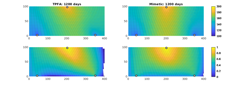
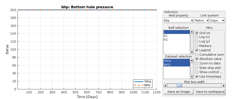
Heterogeneous quarter five-spot: temporal splitting errors
Generated from splittingErrorQ5het.m
In this example, we use a heterogeneous quarter five-spot with petrophysical data sampled from the topmost layer of the SPE 10 data set as an example to illustrate splitting errors that may arise when using a sequential solution procedure. We consider three different mobility ratios: an unfavorable, equal mobilities, and favorable.
mrstModule add incomp spe10 ad-core
Set up model and parameters
dims = [60 120 1];
domain = dims.*[20 10 2]*ft;
G = computeGeometry(cartGrid(dims,domain));
rock = getSPE10rock((1:dims(1)),(1:dims(2))+60,1);
rock.poro = max(rock.poro,.0005);
pv = poreVolume(G,rock);
gravity reset off
rate = sum(poreVolume(G,rock));
W = addWell([],G, rock, 1, 'Type', 'rate', ...
'Val', rate, 'name', 'I', 'radius', .1, 'Comp_i', [1 0]);
W = addWell(W,G, rock, G.cells.num, 'Type', 'rate', ...
'Val', -rate, 'name', 'P', 'radius', .1, 'Comp_i', [0 1]);
hT = computeTrans(G, rock);
x0 = initState(G,W,100*barsa, [0 1]);
Self convergence with respect to time step
For the first test, we illustrate difference in self convergence as a function of mobility ratio M = muw/muo for M=0.1, 1, and 10. These cases have a leading displacement profile that moves faster than the Darcy velocity by a factor rvel=1/(2M(sqrt((M+1)/M)-1)). For each mobility ratio, we set up a simulation that would take 2^m time splitting steps to reach 0.5 PVI for m=1:6. However, to get saturation profiles that cover a more similar portion of the reservoir, we scale the end time for M=0.1 and M=10 by rvel(1)/rvel(M). The self convergence is measured relative to a solution that would have used 256 steps to get to 0.5 PVI.
mu = [1 10; 1 1 ; 10 1];
rvel = @(M) 1./(2.*M.*(sqrt((M+1)./M)-1));
tscale = rvel(mu(:,1)./mu(:,2));
tscale = tscale(2)./tscale;
T = 0.5;
% Prepare plotting
set(gcf,'Position',[200 550 1240 480]);
cval = linspace(0,1,11);
cval = .5*cval(1:end-1)+.5*cval(2:end);
plotData = @(x) ...
contourf(reshape(G.cells.centroids(:,1), G.cartDims),...
reshape(G.cells.centroids(:,2), G.cartDims), ...
reshape(x.s(:,1),G.cartDims), [cval 1]);
colormap(flipud(.5*jet(10)+.5*ones(10,3)));
% Loop over all three viscosity ratios
err = zeros(3,6);
for n=1:3
fluid = initSimpleFluid('mu', mu(n,:).* centi*poise, ...
'rho', [1000,1000].*kilogram/meter^3, 'n', [2 2]);
for m=[8 1:6]
% Time loop
[x,dt,t,tend] = deal(x0, T*2^(-m), 0, tscale(n)*T);
while t<tend
x = incompTPFA(x, G, hT, fluid, 'wells', W);
[tl,dtl,tle] = deal(0,T/2^8, min(tend-t,dt));
while tl < tle
x = implicitTransport(x, G, dtl, rock, fluid, 'wells', W);
tl = tl+dtl;
end
t = t+dt;
end
% Compute discrepancy from reference solution
if m==8
sref = x.s(:,1); snorm = sum(abs(sref).*pv);
else
err(n,m) = sum(abs(x.s(:,1)-sref).*pv)/snorm;
end
% Plot contour plot of solution
subplot(3,7,sub2ind([7,3],min(m,7),n))
plotData(x); axis equal; axis([0 domain(1) 0 domain(2)]);
if n==1
title(sprintf('%d steps',2^m));
else
pos=get(gca,'position');
set(gca,'position',pos+(n-1).*[0 .05 0 0]);
end
set(gca,'XTick',[],'YTick',[]);
drawnow;
end
end
% Plot convergence
figure
semilogy(err','o-','MarkerSize',7,'MarkerFaceColor',[.8 .8 .8],'LineWidth',1);
set(gca,'XTick',1:6,'XTickLabel',{2.^(1:6)}); legend('1:10','1:1','10:1');
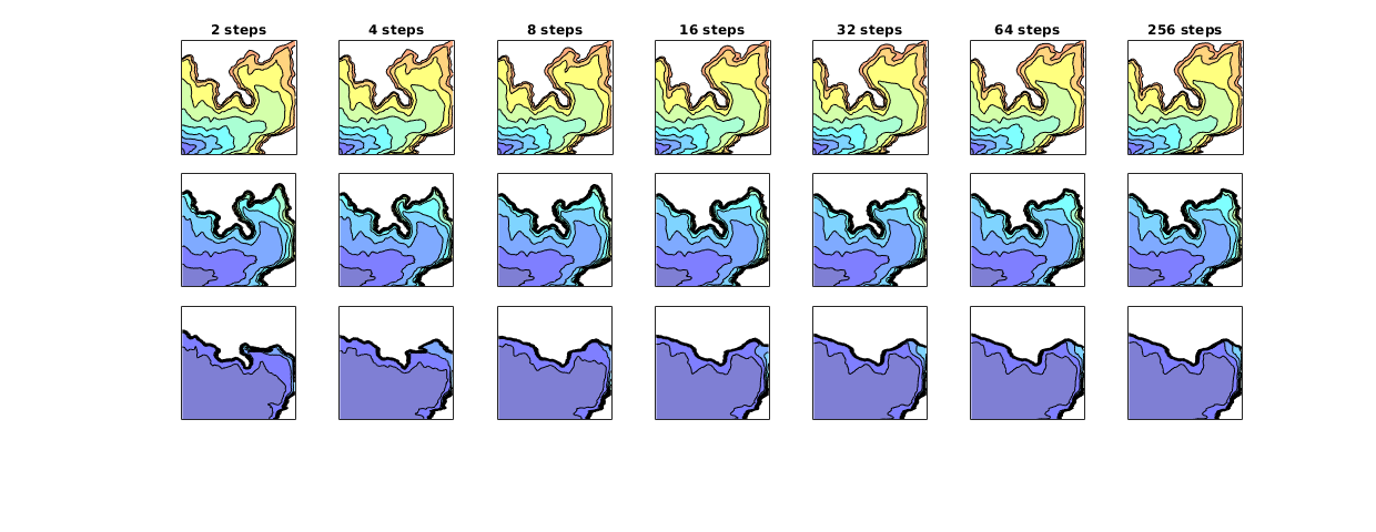
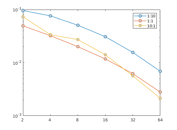
Well curves convergence
We repeate the same simulation as above, except that we continue until 1.5 PVI for all three mobility ratios. We run simulations with constant time-step length (3*4^[0:4] steps) and with a rampup.
Tn = 1.5;
% Constant time step
nstep = [1 4 16 64 256];
dt = T/nstep(end);
wellSols = cell(nstep(end),numel(nstep),3);
% Rampup
dT = repmat(T/32, Tn/T*32,1);
dT = [dT(1)*sort(repmat((2.^-[1:4 4])',2,1)); dT(3:end)];
wSol = cell(numel(dT),3);
for n=1:3
fprintf('Fluid %d: ', n);
fluid = initSimpleFluid('mu', mu(n,:).* centi*poise, ...
'rho', [1000,1000].*kilogram/meter^3, 'n', [2 2]);
for k=1:numel(nstep)
x = x0;
ws = 1;
fprintf('%d,', nstep(k));
for i=1:nstep(k)*Tn/T
x = incompTPFA(x, G, hT, fluid, 'wells', W);
for m=1:nstep(end)/nstep(k)
x = implicitTransport(x, G, dt, rock, fluid, 'wells', W);
wellSols{ws,k,n} = getWellSol(W, x, fluid); ws = ws+1;
end
end
end
fprintf('rampup\n');
x = x0;
for i=1:numel(dT)
x = incompTPFA(x, G, hT, fluid, 'wells', W);
x = implicitTransport(x, G, dT(i), rock, fluid, 'wells', W);
wSol{i,n} = getWellSol(W, x, fluid);
end
end
Fluid 1: 1,4,16,64,256,rampup
Fluid 2: 1,4,16,64,256,rampup
Fluid 3: 1,4,16,64,256,rampup
n = 2;
[tws,dsn,t] = deal(cell(1,numel(nstep)+1));
for i=1:numel(nstep)
tws(i) = {vertcat(wellSols(:,i,n))};
t(i) = {cumsum(dt*ones(Tn/T*nstep(end),1))};
dsn(i) = {num2str(nstep(i))};
end
tws(end) = {vertcat(wSol(:,n))};
t(end) = {cumsum(dT)};
dsn(end) = {'rampup'};
plotWellSols(tws,t, 'datasetnames', dsn);
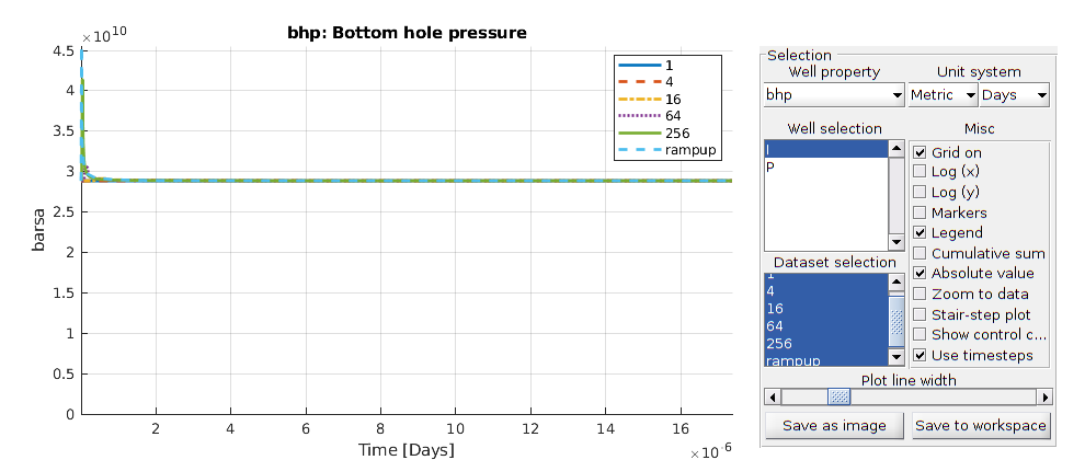
Quarter five-spot: Illustration of temporal splitting errors
Generated from splittingErrorQ5hom.m
We use the standard quarter five-spot test case to illustrate splitting errors that may arise when using a sequential solution procedure to simulate multiphase flow
mrstModule add book incomp diagnostics
Set up model
T = 1;
cartDim = [128 128 1];
gravity reset off
fluid = initSimpleFluid('mu' , [ 1, 1] .* centi*poise , ...
'rho', [1000, 850] .* kilogram/meter^3, ...
'n' , [ 2, 2]);
domain = [250 250 20];
G = computeGeometry(cartGrid(cartDim,domain));
rock = makeRock(G, 450*milli*darcy, 0.2);
rate = .6*sum(poreVolume(G,rock))/T;
W = addWell([],G, rock, 1, 'Type', 'rate', ...
'Val', rate, 'name', 'I', 'radius', .1, 'Comp_i', [1 0]);
W = addWell(W,G, rock, G.cells.num, 'Type', 'rate', ...
'Val', -rate, 'name', 'P', 'radius', .1, 'Comp_i', [0 1]);
hT = computeTrans(G, rock);
Compute reference solution
xr = initState(G,W,100*barsa, [0 1]);
for n=1:128
xr = incompTPFA(xr, G, hT, fluid, 'wells', W);
xr = explicitTransport(xr, G, T/128, rock, fluid, 'wells', W);
end
pv = poreVolume(G,rock);
l1s = norm(xr.s(:,1).*pv,1);
l2p = norm(xr.pressure.^2.*pv, 1);
Contrast multiphase displacement with single-phase time lines
For Corey exponent 2 and equal viscosities, the displacement front will propagate at a speed of a=1/(2(sqrt(2)-1)) relative to the total velocity. Compute the countour showing the position of the displacement front at time 0.6 PVI.
a = 1/(2*(sqrt(2)-1));
x = initState(G,W,100*barsa, [0 1]);
x = incompTPFA(x, G, hT, fluid, 'wells', W);
tau = computeTimeOfFlight(x, G, rock, 'wells', W);
figure('Position',[300 550 1100 300]);
C = contour(reshape(G.cells.centroids(:,1), G.cartDims),...
reshape(G.cells.centroids(:,2), G.cartDims), ...
reshape(tau/T,G.cartDims), a, '-k','LineWidth',1); clf

Run simulation with different time steps
Finally, we compute the multiphase flow solution at time 0.6 PVI using a sequence of increasing splitting time steps. As the number of splitting steps increases, the approximate solution gradually approaches the correct solution computable on this grid
nval = 10;
cval = linspace(0,1,nval+1); cval=.5*cval(1:end-1)+.5*cval(2:end);
colormap(flipud(.5*jet(nval)+.5*ones(nval,3)));
err = nan(7,2);
for n=0:6
nstep = 2^n;
x = initState(G,W,100*barsa, [0 1]);
for i=1:nstep
x = incompTPFA(x, G, hT, fluid, 'wells', W);
x = explicitTransport(x, G, T/nstep, rock, fluid, 'wells', W);
end
err(n+1,1) = norm((xr.s(:,1) - x.s(:,1)).*pv, 1)/l1s;
err(n+1,2) = norm((xr.pressure - x.pressure).^2.*pv, 1)/l2p;
if rem(n,2), continue, end
subplot(1,4,n/2+1);
contourf(reshape(G.cells.centroids(:,1), G.cartDims),...
reshape(G.cells.centroids(:,2), G.cartDims), ...
reshape(x.s(:,1),G.cartDims), [0 cval 1], 'EdgeColor','none');
hold on, plot(C(1,2:end),C(2,2:end),'k-','LineWidth',1); hold off
axis equal; axis([0 domain(1) 0 domain(2)]); caxis([0 1]);
title([num2str(nstep) ' steps'])
set(gca,'XTick',[],'YTick',[]);
drawnow;
end
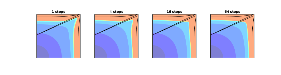
Show convergence table
convrate = log(bsxfun(@rdivide,err(1:end-1,:),err(2:end,:)))./log(2);
convrate = [nan nan; convrate];
clc
fprintf('\n\t L1(S) rate\t L2(p) rate\n');
fprintf('\t-----------------------------------------\n');
fprintf('\t%.3e %.2f \t%.3e %.2f\n', ...
[err(:,1),convrate(:,1),err(:,2),convrate(:,2)]');
fprintf('\t-----------------------------------------\n');
L1(S) rate L2(p) rate
-----------------------------------------
5.570e-02 NaN 4.946e-03 NaN
4.364e-02 0.35 5.052e-04 3.29
2.770e-02 0.66 1.497e-04 1.76
1.434e-02 0.95 4.187e-05 1.84
6.255e-03 1.20 1.046e-05 2.00
...
Heterogeneous quarter five-spot
Generated from viscousFingeringQ5.m
In this example, we will study a heterogeneous quarter five-spot with petrophysical data sampled from the SPE 10 benchmark. We compare fingering effects in a quarter five-spot problem as function of viscosity ratio. We show that an unfavorable mobility ratio (viscosity of injected water is less than the viscosity of the resident oil) leads to pronounced fingers, whereas a piston-like displacement with minimal fingering effects is observed for a favorable mobility ratio.
mrstModule add incomp ad-core spe10
Set up model and parameters
T = 20*year;
dims = [60 120 1];
domain = dims.*[20 10 2]*ft;
G = computeGeometry(cartGrid(dims,domain));
rock = getSPE10rock((1:dims(1)),(1:dims(2))+60,1);
rock.poro = max(rock.poro,.0005);
gravity reset off
rate = sum(poreVolume(G,rock))/T;
W = addWell([],G, rock, 1, 'Type', 'rate', ...
'Val', rate, 'name', 'I', 'radius', .1, 'Comp_i', [1 0]);
W = addWell(W,G, rock, G.cells.num, 'Type', 'rate', ...
'Val', -rate, 'name', 'P', 'radius', .1, 'Comp_i', [0 1]);
hT = computeTrans(G, rock);
x0 = initState(G,W,100*barsa, [0 1]);
cval = linspace(0,1,11); cval=.5*cval(1:end-1)+.5*cval(2:end);
Compare fingering effects
We compute solutions for three different viscosity ratios, mu_w : mu_o = N, for N=10, 1, and 1/10.
set(gcf,'Position',[250 150 1100 660]);
plotData = @(x) ...
contourf(reshape(G.cells.centroids(:,1), G.cartDims),...
reshape(G.cells.centroids(:,2), G.cartDims), ...
reshape(x.s(:,1),G.cartDims), [cval 1]);
colormap(flipud(.5*jet(10)+.5*ones(10,3)));
[N,M] = deal(10,200);
mu = [1 N; 1 1 ; N 1];
[dt,dT] = deal(zeros(M,1), T/M);
is = 1;
wellSol = cell(M,3);
oip = zeros(M,3);
for n=1:3
fluid = initSimpleFluid('mu', mu(n,:).* centi*poise, ...
'rho', [1000,1000].*kilogram/meter^3, 'n', [2 2]);
[x,ip] = deal(x0,1);
for i=1:M
x = incompTPFA(x, G, hT, fluid, 'wells', W);
x = implicitTransport(x, G, dT, rock, fluid, 'wells', W);
dt(i) = dT;
oip(i,n) = sum(x.s(:,2).*poreVolume(G,rock));
wellSol{i,n} = getWellSol(W,x, fluid);
if ~mod(i,40) && ip<=5
subplot(3,5,is); ip=ip+1; is=is+1;
plotData(x); axis equal; axis([0 domain(1) 0 domain(2)]);
set(gca,'XTick',[],'YTick',[]);
if n==1
title(sprintf('%.0f years', sum(dt)/year));
else
set(gca,'position',get(gca,'position')+(n-1)*[0 .05 0 0]);
end
drawnow;
end
end
end
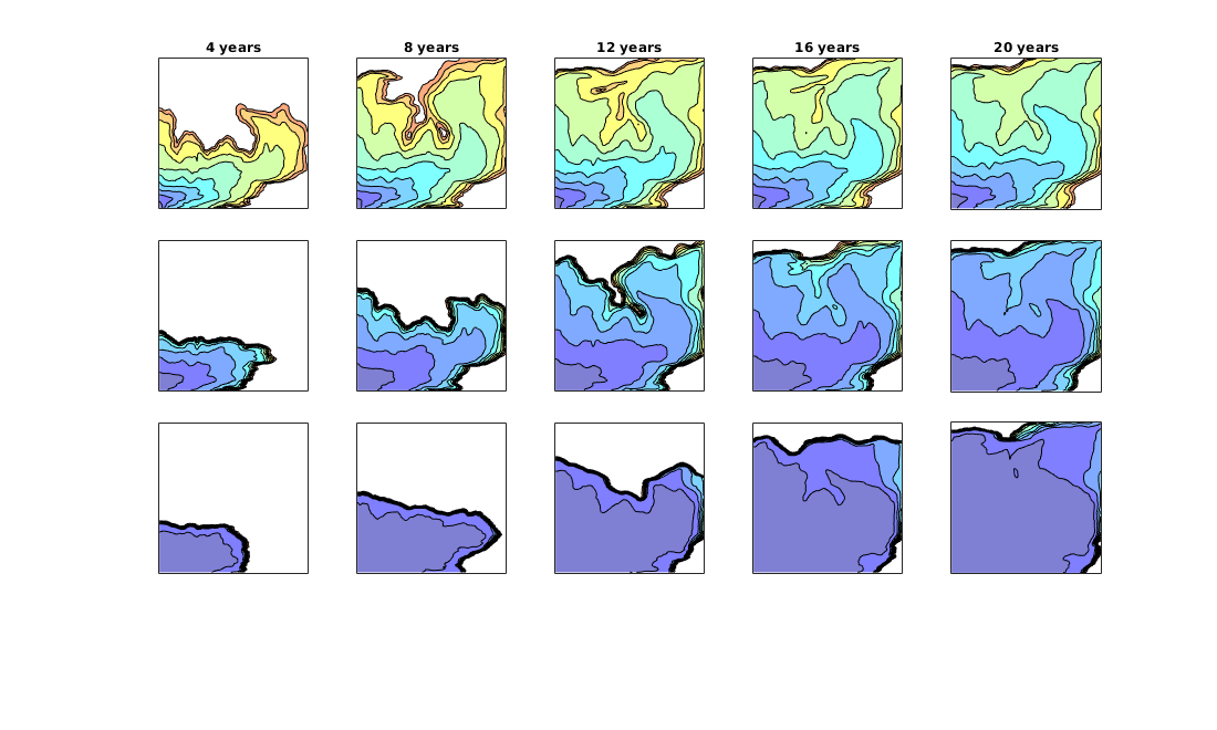
Plot well responses
This plotting only works for predefined quantities like surface rates, bottom-hole pressure, etc. If the well structure contains other quantities, these will appear in the list of available fields but cannot be plotted.
plotWellSols({wellSol(:,1),wellSol(:,2),wellSol(:,3)},...
cumsum(dt),'datasetnames',{'Ratio 1:10','Ratio 1:1','Ratio 10:1'});
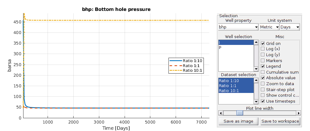
n = 5000000;
pt = randn(n,3);
tic
I = sum(bsxfun(@times, pt>0, [1 2 4]),2)+1;
num = accumarray(I,1);
toc
Elapsed time is 0.149304 seconds.
tic
avg = zeros(8,3);
for j=1:size(pt,1)
quad = sum((pt(j,:)>0).*[1 2 4])+1;
avg(quad,:) = avg(quad,:)+pt(j,:);
end
avg = bsxfun(@rdivide, avg, num);
toc
Elapsed time is 9.847593 seconds.
tic
avg = bsxfun(@rdivide, sparse(I,1:n,1)*pt, accumarray(I,1));
toc
Elapsed time is 0.249902 seconds.
tic
avg = sparse(I,1:n,1)*[pt, ones(n,1)];
avg = bsxfun(@rdivide, avg(:,1:end-1), avg(:,end));
toc
Elapsed time is 0.297510 seconds.
Simple formula using two scalars
Generated from introToAD.m
Compute z = 3 exp(-xy) and its partial derivatives wrt x and y. First, we compute it manually and then using automatic differentiation (AD). To understand what is going on behind the curtains when using AD, you can set a breakpoint at line 13 and use the ‘Step into’ function to step through the different functions that are invoked when evaluating z
[x,y]=deal(1,2);
disp('Manually computed:')
disp([1 -y -x]*3*exp(-x*y))
disp('Automatic differentiation:')
[x,y] = initVariablesADI(1,2);
z = 3*exp(-x*y)
Manually computed:
0.4060 -0.8120 -0.4060
Automatic differentiation:
z =
ADI with properties:
...
Demonstrate the importance of vectorization
m = 15;
[n,t1,t2,t3,t4] = deal(zeros(m,1));
for i = 1:m
n(i) = 2^(i-1);
xv = rand(n(i),1); yv=rand(n(i),1);
[x,y] = initVariablesADI(xv,yv);
tic, z = xv.*yv; zx=yv; zy = xv; t1(i)=toc;
tic, z = x.*y; t2(i)=toc;
if i<17
tic, for k =1:n(i), z(k)=x(k)*y(k); end; t3(i)=toc;
tic, for k =1:n(i), z(k)=x(k).*y(k); end; t4(i)=toc;
end
fprintf('%7d: %6.5f sec, %6.5f sec, %6.5f sec, %6.5f sec\n', ...
n(i), t1(i), t2(i), t3(i), t4(i))
end
1: 0.00018 sec, 0.00024 sec, 0.00118 sec, 0.00054 sec
2: 0.00052 sec, 0.00018 sec, 0.00150 sec, 0.00100 sec
4: 0.00011 sec, 0.00017 sec, 0.00217 sec, 0.00202 sec
8: 0.00006 sec, 0.00017 sec, 0.00213 sec, 0.00206 sec
16: 0.00060 sec, 0.00055 sec, 0.00460 sec, 0.00456 sec
32: 0.00001 sec, 0.00007 sec, 0.00834 sec, 0.00822 sec
64: 0.00001 sec, 0.00007 sec, 0.01669 sec, 0.01636 sec
128: 0.00001 sec, 0.00010 sec, 0.03507 sec, 0.03493 sec
...
clf, set(gca,'FontSize',14);
loglog(n,t1,'-*',n,t2,'-+',n,t3,'-o',n,t4,'-s','LineWidth',2);
legend('exact formulat','vectorized ADI','for loop and mtimes','for loop and times','Location','NorthWest');
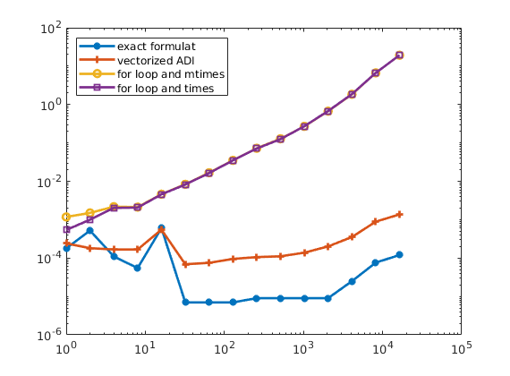
Use automatic differentation to assmble a linear system
First we just evaluate the residual equation as a matrix vector product
x = initVariablesADI(zeros(3,1));
A = [3, 2, -4; 1, -4, 2; -2,- 2. 4];
eq = A*x + [5; 1; -6];
u = -eq.jac{1}\eq.val
u =
1.0000
2.0000
3.0000
Secondly, we can evaluate the equations one by one and then use ADI to assemble the resulting matrix
x = initVariablesADI(zeros(3,1));
eq1 = [ 3, 2, -4]*x + 5;
eq2 = [ 1, -4, 2]*x + 1;
eq3 = [-2,- 2. 4]*x - 6;
eq = cat(eq1,eq2,eq3);
u = -eq.jac{1}\eq.val
u =
1.0000
2.0000
3.0000
Use AD to solve the nonlinear Rosenbrock problem
Problem: minimize f(x,y) = (a-x)^2 + b(y-x^2)^2 = 0 The solution is (a,a^2). A necessary condition for minimum is that grad(f(x,y))=0, which gives two residual equations 2(a-x) - 4bx(y-x^2) = 0 2b(y-x^2) = 0 Here, we set a=1 and b=100
[a,b,tol] = deal(1,100,1e-6);
[x0,incr] = deal([-.5;4]);
while norm(incr)>tol
x = initVariablesADI(x0);
eq = cat( 2*(a-x(1)) - 4*b.*x(1).*(x(2)-x(1).^2), ...
2*b.*(x(2)-x(1).^2));
incr = - eq.jac{1}\eq.val;
x0 = x0 + incr;
end
Slightly more elaborate version with plotting
a,b] = deal(1,100);
fx = @(x) 2*(a-x(1)) - 4*b.*x(1).*(x(2)-x(1).^2);
fy = @(x) 2*b.*(x(2)-x(1).^2);
[tol,res,nit] = deal(1e-6, inf,0);
x = [-.5 4];
while res>tol && nit<100
nit = nit+1;
xd = initVariablesADI(x(end,:)');
eq = cat(fx(xd),fy(xd));
incr = - eq.jac{1}\eq.val;
res = norm(incr);
x = [x; x(end,:)+incr']; %#ok<AGROW>
end
% Plot solution: use modified colormap to clearly distinguish the region
% with lowest colors. Likewise, show the value of f per iteration on a
% nonlinear scale, i.e., f(x,y)^0.1
subplot(4,1,1:3);
f = @(x,y) (a-x).^2 + b.*(y-x.^2).^2;
[xg, yg] = meshgrid(-2:0.2:2, -1.5:0.2:4);
surf(xg,yg,reshape(f(xg(:), yg(:)),size(xg))); shading interp
hold on;
plot3(x(:,1),x(:,2),f(x(:,1),x(:,2)),'-or', 'LineWidth', 2, ...
'MarkerSize',8,'MarkerEdgeColor','k','MarkerFaceColor','r');
hold off
view(-130,45); axis tight; colormap([.3 .3 1; jet(99)]);
subplot(4,1,4)
bar(f(x(:,1),x(:,2)).^.1,'b'); axis tight; set(gca,'YTick',[]);
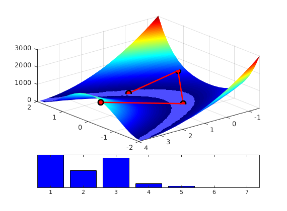
Bed Models 1
Generated from showBedModels.m
pth = getDatasetPath('BedModels1');
fn = dir(fullfile(pth,'*.grdecl'));
for i = 1:numel(fn)
grdecl = readGRDECL(fullfile(pth, fn(i).name));
G = processGRDECL(grdecl);
rock = grdecl2Rock(grdecl,G.cells.indexMap);
clf
if isfield(grdecl,'SATNUM')
q = grdecl.SATNUM(G.cells.indexMap);
else
q = rock.poro;
end
plotCellData(G, q, 'EdgeAlpha',.1, 'EdgeColor','k');
view(3); axis tight off, drawnow
print('-dpng',sprintf('bedmodels1-%d.png', i));
end
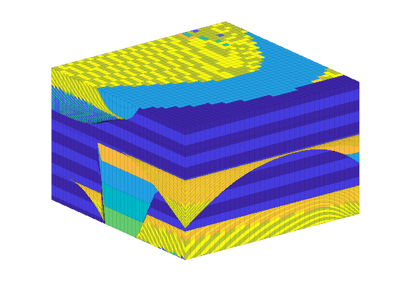
Bed Model 2
grdecl = readGRDECL(fullfile(getDatasetPath('BedModel2'),'BedModel2.grdecl'));
G = processGRDECL(grdecl);
rock = grdecl2Rock(grdecl,G.cells.indexMap);
clf,
plotCellData(G,grdecl.SATNUM(G.cells.indexMap),'EdgeColor','none');
view(3); axis tight off
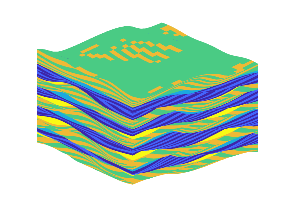
Show fluid models from SPE 1, SPE 3 and SPE 9
Generated from showSPEfluids.m
The purpose of this example is to demonstrate how to read an Eclipse input file, create a fluid model, and inspect it. To this end, we will consider the SPE1, SPE 3, and SPE9 data sets. The example assumes that you have downloaded them already. If not, you should uncomment and run the following line, to bring up the dataset manager that enables you to download the data sets
% mrstDatasetGUI
Read data
If you have used the mrstDatasetGUI functionality to download the SPE 1 and SPE 9 data set, it should be possible to find them on a standard path. We read the data and convert to SI units.
mrstModule add deckformat ad-props ad-core
nr = [1 3 9];
fo = cell(3,1);
col = lines(3);
name = cell(3,1);
decks = cell(3,1);
for i=1:3
name{i} = sprintf('spe%d',nr(i));
pth = getDatasetPath(name{i});
fn = fullfile(pth, sprintf('BENCH_SPE%d.DATA',nr(i)));
decks{i} = readEclipseDeck(fn);
decks{i} = convertDeckUnits(decks{i});
fo{i} = initDeckADIFluid(decks{i});
if ~isfield(fo{i},'sWcon')
fo{i}.sWcon = 0.0;
end
fo{i} = assignRelPerm(fo{i});
end
Plot two-phase relative permeability curves
For a three-phase model we have four relative permeability curves. One for both gas and water and two curves for the oil phase. The oil relative permeability is tabulated for both water-oil and oil-gas systems.
s = linspace(0,1,51)';
for i=1:numel(name), name{i} = upper(name{i}); end
figure; hold all, set(gca,'FontSize',14)
for i=1:3
plot(s, fo{i}.krW(s), 'linewidth', 2, 'Color',col(i,:))
end
grid on
legend(name{:},'Location','NorthWest');
xlabel('Water saturation');
title('Water relative permeability curve')
figure; hold all, set(gca,'FontSize',14)
for i=1:3
krOW = fo{i}.krOW(s); krOW(s>1-fo{i}.sWcon)=nan;
krOG = fo{i}.krOG(s); krOG(s>1-fo{i}.sWcon)=nan;
plot(s, krOW, '-','Color',col(i,:), 'linewidth',2);
plot(s, krOG, '--', 'linewidth', 4, 'Color',col(i,:))
end
grid on
h = findobj(gca,'Type','line');
legend(h([6 5 6 4 2]),'oil/water system', 'oil/gas system', name{:}, ...
'Location', 'NorthWest');
xlabel('Oil saturation');
title('Oil relative permeability curves')
figure; hold all, set(gca,'FontSize',14)
for i=1:3
krG = fo{i}.krG(s); krG(s>1-fo{i}.sWcon)=nan;
plot(s, krG, 'linewidth', 2,'Color',col(i,:))
end
grid on
legend(name{:},'Location','SouthEast');
xlabel('Gas saturation');
title('Gas relative permeability curve')
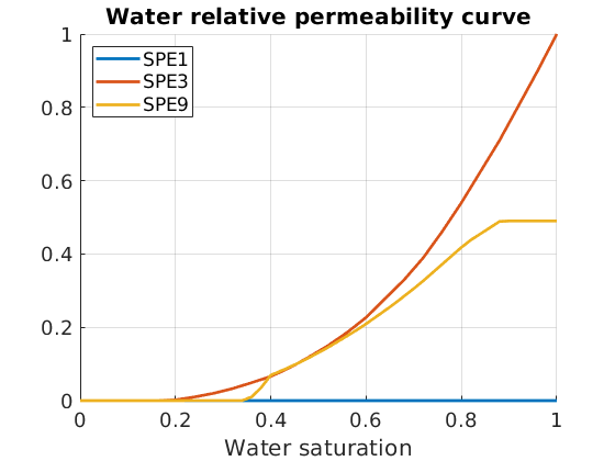
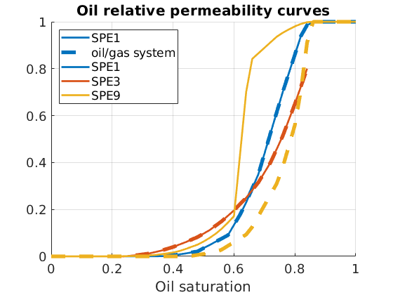
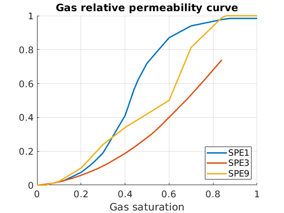
Plot three-phase relative permeability for oil
When all three phases are present simultaneously in a single cell, we need to use some functional relationship to combine the two-phase curves in a reasonable manner, resulting in a two-dimensional relative permeability model. Herein, we use a simple linear interpolation, which is also the default in Eclipse
[sw, sg] = meshgrid(linspace(0,1,201));
so=1-sw-sg;
for i=1:3
[~, krO] = fo{i}.relPerm(sw(:),sg(:));
krO = reshape(krO,size(sw)); krO(sw+sg>1)=nan;
figure; set(gca,'FontSize',14);
[mapx,mapy] = ternaryAxis('names',{'S_w';'S_g';'S_o'},'FontSize',14);
contourf(mapx(sw,sg,so), mapy(sw,sg,so), krO, 20)
set(gca,'YLim',[0 sqrt(3)/2]);
text(mapx(.45,.45,.1),mapy(.45,.45,.1),'Oil relative permeability', ...
'BackgroundColor','w','HorizontalAlignment','center','FontSize',14);
caxis([0 1]);
end
% =========================================================================
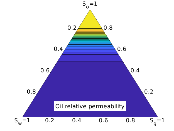
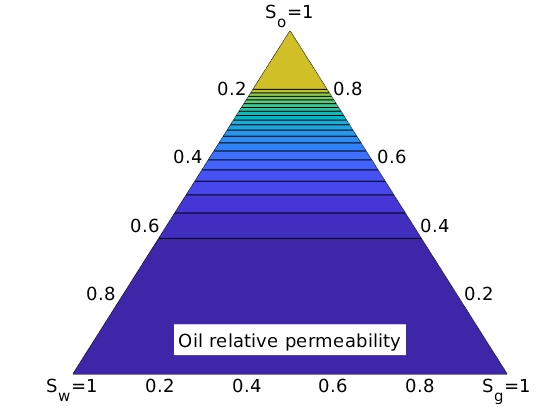
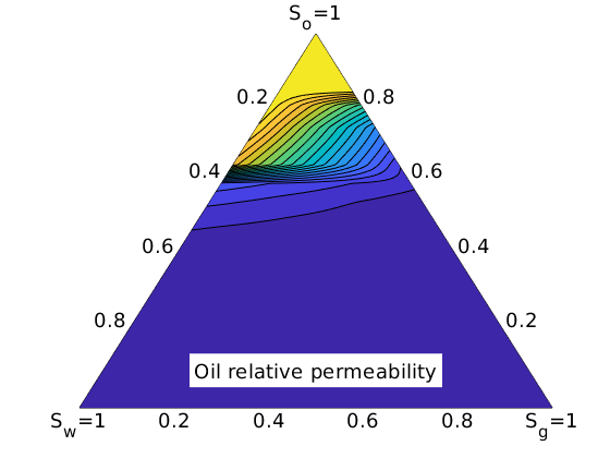
Phase behavior of live oil for the SPE 1 or SPE 9 model
In the following, we will briefly show the phase behavior for gas and oil in the model. That is, we will show both the input data points and the interpolated data obtained from the functions in the fluid object
% Set input deck and fluid object
[deck, f] = deal(decks{1}, fo{1});
% Extract data from the input deck
pvto = deck.PROPS.PVTO{1};
rsd = pvto.key([1:end end]);
pbp = pvto.data([pvto.pos(1:end-1)' end],1);
Bod = pvto.data([pvto.pos(1:end-1)' end],2);
muOd = pvto.data([pvto.pos(1:end-1)' end],3);
Plot Rs
figure, set(gca,'FontSize',14)
pargs = {'LineWidth', 2, 'MarkerSize',7,'MarkerFaceColor',[.5 .5 .5]};
plot(pbp/barsa,rsd,'-o',pargs{:}); xlabel('Pressure [bar]');
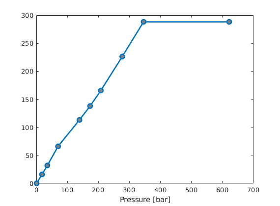
Plot oil formation-volume factor and viscosity for oil
For Bo, we plot both the tabulated data as well as interpolated data at various combinations of dissolved gas and reservoir pressures. For each data point, we must first determine whether the state is saturated or not by comparing the actual amount of dissolved gas against the maximum possible amount of solved gas for this pressure.
[M, N] = deal(11,51);
[RsMax,pMax] = deal(max(rsd), max(pbp));
[rs,p] = meshgrid(linspace(10,RsMax-10,M), linspace(0,pMax,N));
Rv = reshape(f.rsSat(p(:)), N, M);
isSat = rs >= Rv;
rs(isSat) = Rv(isSat);
Bo = 1./reshape(f.bO(p(:), rs(:), isSat(:)),N,M);
muO = reshape(f.muO(p(:), rs(:), isSat(:)),N,M);
% Formation-volume factor
figure, hold on, set(gca,'FontSize',14)
for j=1:M
i = isSat(:,j);
plot(p(i,j)/barsa, Bo(i,j),'b-',p(~i,j)/barsa,Bo(~i,j),'-r');
end
plot(pbp/barsa,Bod,'-bo',pargs{:});
hold off, axis tight, xlabel('Pressure [bar]');
title('Oil formation-volume factor [-]');
% Viscosity
figure, hold on, set(gca,'FontSize',14)
for j=1:M
i = isSat(:,j);
plot(p(i,j)/barsa, convertTo(muO(i,j), centi*poise),'b-',...
p(~i,j)/barsa, convertTo(muO(~i,j), centi*poise),'-r');
end
plot(pbp/barsa, convertTo(muOd, centi*poise),'-bo',pargs{:});
hold off, axis tight, xlabel('Pressure [bar]');
title('Oil viscosity [cP]');
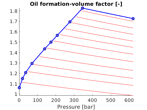
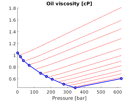
Phase behavior for the dry gas (SPE 1 or SPE9)
pvdg = deck.PROPS.PVDG{1};
figure, set(gca,'FontSize',14);
plot(pvdg(:,1)/barsa,pvdg(:,2),'-o',pargs{:})
set(gca,'YScale','log')
xlabel('Pressure [bar]');
title('Gas formation-volume factor [-]');
figure, set(gca,'FontSize',14);
plot(pvdg(:,1)/barsa,convertTo(pvdg(:,3), centi*poise), '-o',pargs{:})
xlabel('Pressure [bar]');
title('Gas viscosity [cP]');
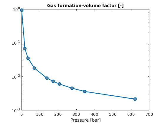
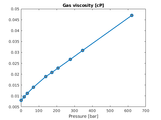
Show inconsistencies for large pressures (only SPE1)
For sufficintly high pressure/gas-oil ratios, the interpolated shrinkage factors will cross zero, which causes blowup and negative Bo values. In turn, this leads to negative partial volumes.
[M, N] = deal(101,201);
[rs,p] = meshgrid(linspace(f.rsSat(100*barsa),f.rsSat(1300*barsa),M), ...
linspace(100,1300,N)*barsa);
Rv = reshape(f.rsSat(p(:)), N, M);
isSat = rs >= Rv;
rs(isSat) = Rv(isSat);
bo = reshape(f.bO (p(:), rs(:), isSat(:)),N,M);
Bo = 1./bo;
muO = reshape(f.muO(p(:), rs(:), isSat(:)),N,M);
bg = reshape(f.bG (p(:)), N, M);
Bg = 1./bg;
figure
contourf(p/barsa,rs,bo,[-inf linspace(-.2,.9,12) inf]); axis tight
set(gca,'FontSize',20); xlabel('Pressure [bar]'); ylabel('Gas-oil ratio');
cb = colorbar; set(cb,'FontSize',20);
colormap(repmat([linspace(.2,.3,4) linspace(.6,1,20)]',1,3));
figure
contourf(p/barsa,rs,1./bo - rs./bg,[-inf linspace(-10,10,41) inf]); axis tight
set(gca,'FontSize',20); xlabel('Pressure [bar]');ylabel('Gas-oil ratio');
caxis([-10,10]); cb = colorbar; set(cb,'FontSize',20);
colormap(repmat([linspace(.25,.5,20) linspace(.7,.95,20)]',1,3));
% =========================================================================
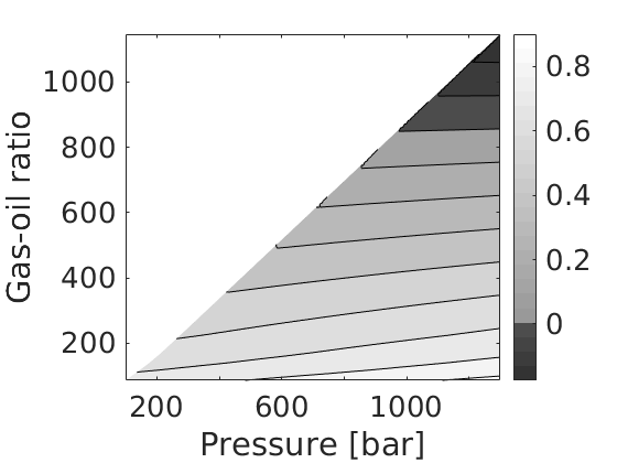
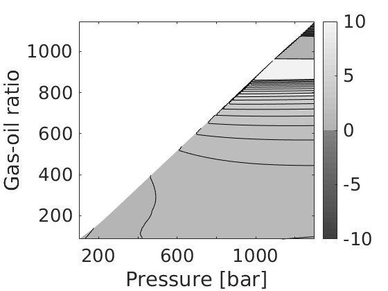
Dead oil and gas with vaporized oil (SPE3)
The SPE 3 benchmark was designed to study gas cycling in a rich�?gas reservoir with retrograde condensation. The original setup was for compositional simulation. The current input file describes a black-oil translation of the compositional model. into a
[deck, f] = deal(decks{2}, fo{2});
pvdo = deck.PROPS.PVDO{1};
figure, set(gca,'FontSize',14);
pargs = {'LineWidth', 2, 'MarkerSize',7,'MarkerFaceColor',[.5 .5 .5]};
plot(pvdo(:,1)/barsa, pvdo(:,2),'-o',pargs{:})
xlabel('Pressure [bar]');
title('Oil formation-volume factor [-]');
figure, set(gca,'FontSize',14);
plot(pvdo(:,1)/barsa, convertTo(pvdo(:,3), centi*poise), '-o',pargs{:})
xlabel('Pressure [bar]');
title('Oil viscosity [cP]');
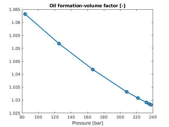
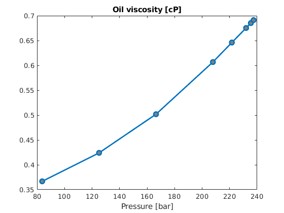
Rich gas with retrograde condensation
Extract data from the input deck
pvtg = deck.PROPS.PVTG{1};
pbp = convertTo(pvtg.key,barsa);
rvd = pvtg.data([1 pvtg.pos(2:end-1)'],1);
Bgd = pvtg.data(:,2);
muGd = convertTo(pvtg.data(:,3), centi*poise);
p = pvtg.key(rldecode((1:numel(pvtg.key))',diff(pvtg.pos),1))/barsa;
Plot Rv
figure, set(gca,'FontSize',14)
hold on
for i=1:numel(pbp)
ind = pvtg.pos(i):pvtg.pos(i+1)-1;
plot(p(ind),pvtg.data(ind,1),'-ok',...
'MarkerSize',6,'MarkerFaceColor',[.5 .5 .5]);
end
plot(pbp,rvd,'-o',pargs{:}); xlabel('Pressure [bar]');
title('Maximum vaporized oil-gas ratio [-]');
hold off
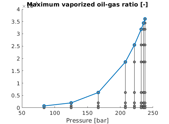
Plot Bg
figure, set(gca,'FontSize',14)
plot(pbp,Bgd([pvtg.pos(2:end-1)'-1 end]),'-r', ...
pbp, Bgd(pvtg.pos(1:end-1)), '-bo', pargs{:});
xlabel('Pressure [bar]');
title('Gas formation-volume factor [-]');
% Make inset
axes('position',[.48 .45 .4 .4]);
hold on
for i=1:numel(pbp)
ind = pvtg.pos(i):pvtg.pos(i+1)-1;
plot(p(ind),pvtg.data(ind,2),'-ok',...
'MarkerSize',6,'MarkerFaceColor',[.5 .5 .5]);
end
plot(pbp,Bgd([pvtg.pos(2:end-1)'-1 end]),'-r', ...
pbp, Bgd(pvtg.pos(1:end-1)), '-bo', pargs{:});
hold off
axis([205 240 4.2e-3 4.8e-3]);
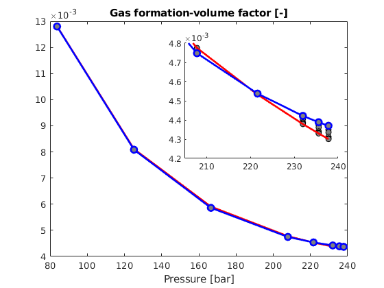
Plot gas density
bG = f.bG(p*barsa, pvtg.data(:,1), false(size(p)));
rho = bG*f.rhoGS + bG.*pvtg.data(:,1)*f.rhoOS;
figure, hold on, set(gca,'FontSize', 14)
for i=1:numel(pbp),
ind = pvtg.pos(i):pvtg.pos(i+1)-1;
plot(p(ind),rho(ind),'-ok',...
'MarkerSize',6,'MarkerFaceColor',[.5 .5 .5]);
end
plot(pbp,rho([pvtg.pos(2:end-1)'-1 end]),'-or', ...
pbp, rho(pvtg.pos(1:end-1)), '-bo', pargs{:});
hold off
xlabel('Pressure [bar]'); title('Density of gaseous phase [kg/m3]');
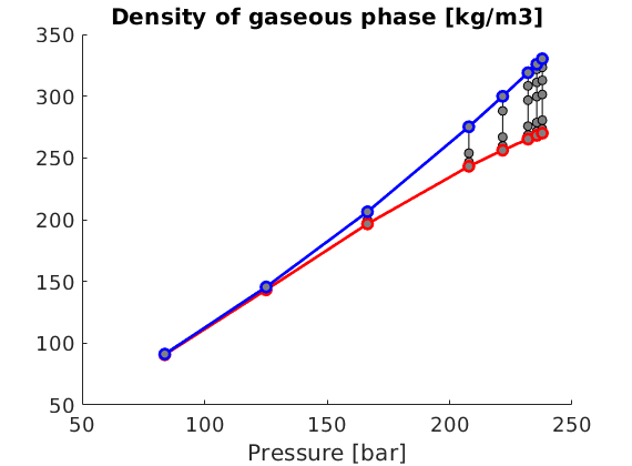
Plot muG
figure, hold on, set(gca,'FontSize',14)
for i=1:numel(pbp)
ind = pvtg.pos(i):pvtg.pos(i+1)-1;
plot(p(ind), muGd(ind), '-ok',...
'MarkerSize',6,'MarkerFaceColor',[.5 .5 .5] );
end
plot(pbp,muGd([pvtg.pos(2:end-1)'-1 end]),'-or', ...
pbp, muGd(pvtg.pos(1:end-1)), '-ob',pargs{:});
hold off
xlabel('Pressure [bar]');
title('Gas viscosity [cP]');
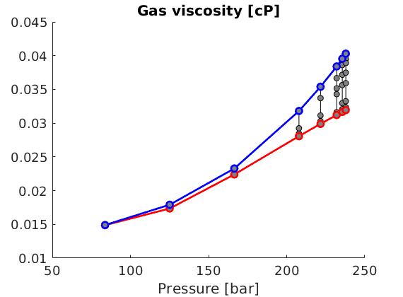
Interpolation/extrapolation of viscosity
For sufficintly high pressure/gas-oil ratios, the interpolated viscosity values exhibit unphysical behavior
[M, N] = deal(51,51);
[rs,pp] = meshgrid(linspace(0,f.rvSat(240*barsa),M), ...
linspace(200,240,N)*barsa);
Rv = reshape(f.rvSat(pp(:)), N, M);
isSat = rs >= Rv;
rs(isSat) = Rv(isSat);
muG = reshape(f.muG(pp(:), rs(:), isSat(:)),N,M);
figure;
contourf(pp/barsa,rs,convertTo(muG,centi*poise),21);
hold on
p = pvtg.key(rldecode((1:numel(pvtg.key))',diff(pvtg.pos),1))/barsa;
for i=1:numel(pbp)
ind = pvtg.pos(i):pvtg.pos(i+1)-1;
plot(p(ind),pvtg.data(ind,1),'-ok',...
'MarkerSize',6,'MarkerFaceColor',[.5 .5 .5]);
end
plot(pbp,rvd,'-o',pargs{:});
hold off
cb = colorbar; set([gca;cb],'FontSize',20); xlabel('Pressure [bar]');
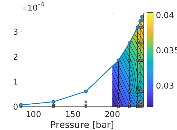
Plot viscosity as function of pressure only for a larger pressure interval
[M, N] = deal(11,21);
[rs,pp] = meshgrid(linspace(0,f.rvSat(280*barsa),M), ...
linspace(160,280,N)*barsa);
Rv = reshape(f.rvSat(pp(:)), N, M);
isSat = rs >= Rv;
rs(isSat) = Rv(isSat);
muG = convertTo(reshape(f.muG(pp(:), rs(:), isSat(:)),N,M),centi*poise);
figure
y = muG; y(isSat)=NaN;
z = muG; z(~isSat) = NaN;
plot(pp/barsa, y,'k--');
hold on
plot(pp/barsa, z, '--k','LineWidth',3);
hold on, set(gca,'FontSize',20)
for i=1:numel(pbp)
ind = pvtg.pos(i):pvtg.pos(i+1)-1;
plot(p(ind), muGd(ind), '-ok',...
'MarkerSize',6,'MarkerFaceColor',[.5 .5 .5] );
end
plot(pbp,muGd([pvtg.pos(2:end-1)'-1 end]),'-ok', ...
pbp, muGd(pvtg.pos(1:end-1)), '-ok',pargs{:});
hold off
xlabel('Pressure [bar]');
axis([160 280 0.015 0.08]);
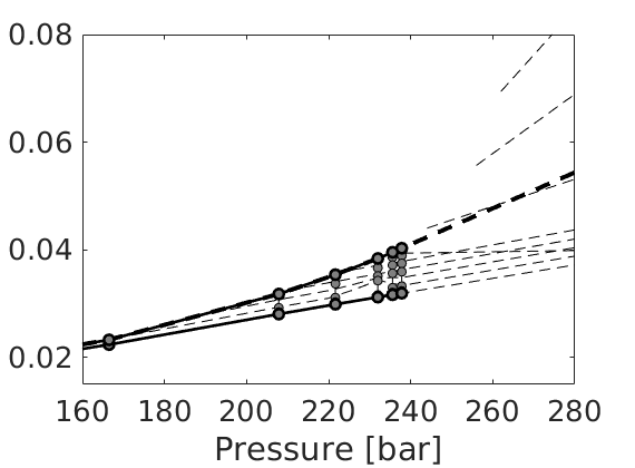
Conceptual three-phase compressible model
Generated from threePhaseAD.m
The purpose of the example is to show how one can implement compressible three-phase flow models using automatic differentiation and the abstract differentiation operators in MRST. To this end, we set up a relatively simple model in which the upper 1/3 is initially filled with gas, the middle 1/3 is filled with oil, and the bottom 1/3 is filled with water. Water is injected in the lower southwest corner and fluids are produced from the northeast corner of the middle layer. To mimic the effect of injector and producer wells, we manipulate the flow equations to ensure reasonable inflow/outflow for the perforated cells. The code can be run with or without water injection. Relative permeabilities are sampled from the SPE3 benchmark. Physical properties are in generally chosen quite haphazardly for illustration purposes. The last plots use ‘hold all’ so that if you run the function twice with or without water injection, the plots of pressures and oil and gas production will be added to the same plots.
mrstModule add ad-core ad-props deckformat
if exist('pvi','var')~=1
pvi = .5;
end
useInj = (pvi>0);
Set up model geometry
[nx,ny,nz] = deal( 11, 11, 3);
[Dx,Dy,Dz] = deal(200, 200, 50);
G = cartGrid([nx, ny, nz], [Dx, Dy, Dz]);
G = computeGeometry(G);
Define rock model
rock = makeRock(G, 30*milli*darcy, 0.2);
cr = 1e-6/psia;
pR = 200*barsa;
pvR = poreVolume(G, rock);
pv = @(p) pvR .* exp(cr * (p - pR) );
Fluid model
Water is slightly compressible with quadratic relative permeability
muW = 1*centi*poise;
cw = 2e-6/psia;
rhoWR = 1014*kilogram/meter^3;
rhoWS = 1000*kilogram/meter^3;
rhoW = @(p) rhoWR .* exp( cw * (p - pR) );
% Oil phase is lighter and has a cubic relative permeability
muO = 0.5*centi*poise;
co = 1e-5/psia;
rhoOR = 850*kilogram/meter^3;
rhoOS = 750*kilogram/meter^3;
rhoO = @(p) rhoOR .* exp( co * (p - pR) );
% Gas
muG = 0.015*centi*poise;
cg = 1e-3/psia;
rhoGR = 1.2;
rhoGS = 1;
rhoG = @(p) rhoGR .* exp( cg * (p - pR) );
% Get relative permeabilities from the SPE3 data set
pth = getDatasetPath('spe3');
fn = fullfile(pth, 'BENCH_SPE3.DATA');
deck = readEclipseDeck(fn);
deck = convertDeckUnits(deck);
f = initDeckADIFluid(deck);
f = assignRelPerm(f);
Extract grid information
nf = G.faces.num; % Number of faces
nc = G.cells.num; % Number of cells
N = double(G.faces.neighbors); % Map: face -> cell
F = G.cells.faces(:,1); % Map: cell -> face
intInx = all(N ~= 0, 2); % Interior faces
N = N(intInx, :); % Interior neighbors
Compute transmissibilities
hT = computeTrans(G, rock); % Half-transmissibilities
T = 1 ./ accumarray(F, 1 ./ hT, [nf, 1]); % Harmonic average
T = T(intInx); % Restricted to interior
nf = size(N,1);
Define discrete operators
D = sparse([(1:nf)'; (1:nf)'], N, ones(nf,1)*[-1 1], nf, nc);
grad = @(x) D*x;
div = @(x)-D'*x;
avg = @(x) 0.5 * (x(N(:,1)) + x(N(:,2)));
upw = @(flag, x) flag.*x(N(:, 1)) + ~flag.*x(N(:, 2));
gradz = grad(G.cells.centroids(:,3));
Impose vertical equilibrium
gravity reset on,
g = norm(gravity);
equil = ode23(@(z,p) g.* rhoO(p), [0, max(G.cells.centroids(:,3))], pR);
p0 = reshape(deval(equil, G.cells.centroids(:,3)), [], 1); clear equil
sW0 = f.sWcon*ones(G.cells.num, 1);
sW0 = reshape(sW0,G.cartDims); sW0(:,:,nz)=1; sW0 = sW0(:);
sG0 = zeros(G.cells.num, 1);
sG0 = reshape(sG0,G.cartDims); sG0(:,:, 1)=1-f.sWcon; sG0 = sG0(:);
ioip = sum(pv(p0).*(1-sW0 - sG0).*rhoO(p0));
igip = sum(pv(p0).*sG0.*rhoG(p0));
Schedule and injection/production
nstep = 108;
Tf = 1080*day;
dt = Tf/nstep*ones(1,nstep);
dt = [dt(1).*sort(repmat(2.^-[1:5 5],1,1)) dt(2:end)];
nstep = numel(dt);
[inRate, inIx ] = deal(pvi*sum(pv(p0))/Tf, nx*ny*nz-nx*ny+1);
[outPres, outIx] = deal(100*barsa, 2*nx*ny);
Initialize for solution loop
[p, sW, sG] = initVariablesADI(p0, sW0, sG0);
[pIx, wIx, gIx] = deal(1:nc, (nc+1):(2*nc), (2*nc+1):(3*nc));
[tol, maxits] = deal(1e-5,15);
pargs = {};% {'EdgeColor','k','EdgeAlpha',.1};
sol = repmat(struct('time',[],'pressure',[], 'sW', [], 'sG', []),[nstep+1,1]);
sol(1) = struct('time', 0, 'pressure', value(p),'sW', value(sW), 'sG', value(sG));
Main loop
t = 0;
hwb = waitbar(t,'Simulation ..');
nits = nan(nstep,1);
i = 1;
for n=1:nstep
t = t + dt(n);
fprintf('\nTime step %d: Time %.2f -> %.2f days\n', ...
n, convertTo(t - dt(n), day), convertTo(t, day));
% Newton loop
resNorm = 1e99;
[p0, sW0, sG0] = deal(value(p), value(sW),value(sG));
nit = 0;
while (resNorm > tol) && (nit <= maxits)
% Densities and pore volumes
[rW,rW0,rO,rO0,rG,rG0] = ....
deal(rhoW(p), rhoW(p0), rhoO(p), rhoO(p0), rhoG(p), rhoG(p0));
[vol, vol0] = deal(pv(p), pv(p0));
% Mobility: Relative permeability over constant viscosity
[krW, krO, krG] = f.relPerm(sW,sG);
mobW = krW./muW;
mobO = krO./muO;
mobG = krG./muG;
% Pressure differences across each interface
dp = grad(p);
dpW = dp-g*avg(rW).*gradz;
dpO = dp-g*avg(rO).*gradz;
dpG = dp-g*avg(rG).*gradz;
% Phase fluxes:
% Density and mobility is taken upwinded (value on interface is
% defined as taken from the cell from which the phase flow is
% currently coming from). This gives more physical solutions than
% averaging or downwinding.
vW = -upw(value(dpW) <= 0, rW.*mobW).*T.*dpW;
vO = -upw(value(dpO) <= 0, rO.*mobO).*T.*dpO;
vG = -upw(value(dpG) <= 0, rG.*mobG).*T.*dpG;
% Conservation of water and oil
water = (1/dt(n)).*(vol.*rW.*sW - vol0.*rW0.*sW0) + div(vW);
oil = (1/dt(n)).*(vol.*rO.*(1-sW-sG) - vol0.*rO0.*(1-sW0-sG0)) + div(vO);
gas = (1/dt(n)).*(vol.*rG.*sG - vol0.*rG0.*sG0) + div(vG);
% Injector: volumetric source term multiplied by surface density
if useInj
water(inIx) = water(inIx) - inRate.*rhoWS;
end
% Producer: replace equations by new ones specifying fixed pressure
% and zero water saturation
oil(outIx) = p(outIx) - outPres;
water(outIx) = sW(outIx);
gas(outIx) = sG(outIx);
% Collect and concatenate all equations (i.e., assemble and
% linearize system)
eqs = {oil, water, gas};
eq = cat(eqs{:});
% Compute Newton update and update variable
res = eq.val;
upd = -(eq.jac{1} \ res);
p.val = p.val + upd(pIx);
sW.val = sW.val + upd(wIx);
%sW.val = max( min(sW.val, 1), 0);
sG.val = sG.val + upd(gIx);
%sG.val = max( min(sG.val, 1), 0);
resNorm = norm(res);
nit = nit + 1;
fprintf(' Iteration %3d: Res = %.4e\n', nit, resNorm);
end
if nit > maxits
error('Newton solves did not converge')
else % plot
nits(n) = nit;
figure(1); clf
subplot(2,1,1)
plotCellData(G, value(p)/barsa, pargs{:});
title('Pressure'), view(30, 40);
subplot(2,1,2)
sg = value(sG); sw = value(sW);
plotCellData(G,[sg, 1-sg-sw, sw]/1.001+1e-4,pargs{:}); % Avoid color artifacts
caxis([0, 1]), view(30, 40); title('Saturation')
drawnow
sol(n+1) = struct('time', t, ...
'pressure', value(p), ...
'sW', value(sW), ...
'sG', value(sG));
waitbar(t/Tf,hwb);
pause(.1);
end
end
close(hwb);
Time step 1: Time 0.00 -> 0.31 days
Iteration 1: Res = 1.0208e+07
Iteration 2: Res = 4.1526e+00
Iteration 3: Res = 9.3067e-01
Iteration 4: Res = 6.8833e-02
Iteration 5: Res = 2.6936e-02
Iteration 6: Res = 6.3870e-02
...
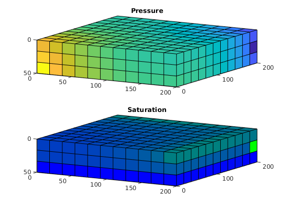
figure(2),
subplot(2,1,2-value(useInj));
bar(nits,1,'EdgeColor','r','FaceColor',[.6 .6 1]);
axis tight, set(gca,'YLim',[0 10]);
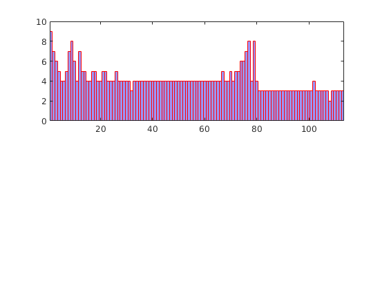
figure(3); hold all
ipr = arrayfun(@(x) x.pressure(inIx), sol)/barsa;
t = arrayfun(@(x) x.time, sol)/day;
fpr = arrayfun(@(x) sum(x.pressure)/G.cells.num, sol)/barsa;
plot(t,ipr,'-', t,fpr, '--');
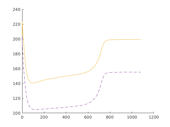
igure(4);
oip = arrayfun(@(x) sum(pv(x.pressure).*(1-x.sW-x.sG).*rhoO(x.pressure)), sol);
gip = arrayfun(@(x) sum(pv(x.pressure).*x.sG.*rhoG(x.pressure)), sol);
subplot(1,2,1), hold all
plot(t,(ioip-oip)./rhoOS)
subplot(1,2,2), hold all
plot(t,(igip-gip)./rhoGS)
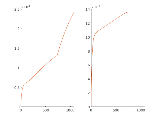
Conceptual two-phase compressible model
Generated from twoPhaseAD.m
The purpose of the example is to show how one can implement compressible multiphase flow models using automatic differentiation and the abstract differentiation operators in MRST. To this end, we set up a relatively simple model in which the upper 2/3 is initially filled with oil and the bottom 1/3 is filled with water. Water is injected in the lower southwest corner and fluids are produced from the upper northeast corner. To mimic the effect of injector and producer wells, we manipulate the flow equations to ensure reasonable inflow/outflow for the perforated cells. The code can be run with compressible or incompressible fluids and rock. (The compressibility of oil is somewhat exaggerated for illustration purposes.) The last plots use ‘hold all’ so that if you run the function twice with compressible/incompressible model, the plots of pressures, condition numbers, and oil production will be added to the same plots.
if exist('isCompr','var')~=1
isCompr = false;
end
Set up model geometry
[nx,ny,nz] = deal( 11, 11, 3);
[Dx,Dy,Dz] = deal(200, 200, 50);
G = cartGrid([nx, ny, nz], [Dx, Dy, Dz]);
G = computeGeometry(G);
figure(1); clf
plotGrid(G); view(3); axis tight
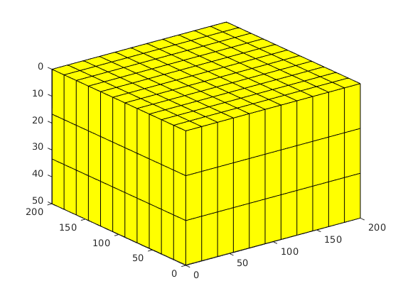
Define rock model
rock = makeRock(G, 30*milli*darcy, 0.2);
cr = 1e-6/psia*double(isCompr);
pR = 200*barsa;
pvR = poreVolume(G, rock);
pv = @(p) pvR .* exp(cr * (p - pR) );
p = linspace(100*barsa,250*barsa,30)';
s = linspace(0,1,50)';
figure(1), clf
plot(p/barsa, pvR(1).*exp(cr*(p-pR)),'LineWidth',2);
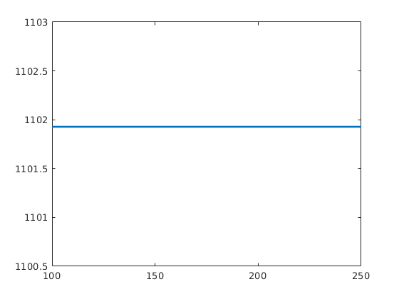
Fluid model
Water is slightly compressible with quadratic relative permeability
muW = 1*centi*poise;
cw = 2e-6/psia*double(isCompr);
rhoWR = 1014*kilogram/meter^3;
rhoWS = 1000*kilogram/meter^3;
rhoW = @(p) rhoWR .* exp( cw * (p - pR) );
krW = @(S) S.^2;
% Oil phase is lighter and has a cubic relative permeability
muO = 5*centi*poise;
co = 1e-5/psia*double(isCompr);
rhoOR = 850*kilogram/meter^3;
rhoOS = 750*kilogram/meter^3;
rhoO = @(p) rhoOR .* exp( co * (p - pR) );
krO = @(S) S.^3;
% Plot compressibility factors
figure(1), subplot(1,2,1)
plot(p/barsa, [rhoW(p), rhoO(p)],'LineWidth',2);
legend('Water density', 'Oil density','Location','best')
% Plot relative permeability
subplot(1,2,2);
plot(s, [krW(s), krO(s)],'LineWidth',2);
legend('krW', 'krO','Location','NorthWest');
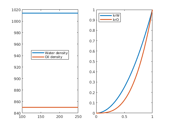
Extract grid information
nf = G.faces.num; % Number of faces
nc = G.cells.num; % Number of cells
N = double(G.faces.neighbors); % Map: face -> cell
F = G.cells.faces(:,1); % Map: cell -> face
intInx = all(N ~= 0, 2); % Interior faces
N = N(intInx, :); % Interior neighbors
Compute transmissibilities
hT = computeTrans(G, rock); % Half-transmissibilities
T = 1 ./ accumarray(F, 1 ./ hT, [nf, 1]); % Harmonic average
T = T(intInx); % Restricted to interior
nf = size(N,1);
Define discrete operators
D = sparse([(1:nf)'; (1:nf)'], N, ones(nf,1)*[-1 1], nf, nc);
grad = @(x) D*x;
div = @(x)-D'*x;
avg = @(x) 0.5 * (x(N(:,1)) + x(N(:,2)));
upw = @(flag, x) flag.*x(N(:, 1)) + ~flag.*x(N(:, 2));
gradz = grad(G.cells.centroids(:,3));
spy(D)
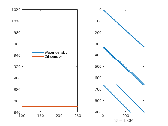
Impose vertical equilibrium
gravity reset on,
g = norm(gravity);
equil = ode23(@(z,p) g.* rhoO(p), [0, max(G.cells.centroids(:,3))], pR);
p0 = reshape(deval(equil, G.cells.centroids(:,3)), [], 1); clear equil
sW0 = zeros(G.cells.num, 1);
sW0 = reshape(sW0,G.cartDims); sW0(:,:,nz)=1; sW0 = sW0(:);
ioip = sum(pv(p0).*(1-sW0).*rhoO(p0));
Schedule and injection/production
nstep = 36;
Tf = 360*day;
dt = Tf/nstep*ones(1,nstep);
dt = [dt(1).*sort(repmat(2.^-[1:5 5],1,1)) dt(2:end)];
nstep = numel(dt);
[inRate, inIx ] = deal(.1*sum(pv(p0))/Tf, nx*ny*nz-nx*ny+1);
[outPres, outIx] = deal(100*barsa, nx*ny);
Initialize for solution loop
[p, sW] = initVariablesADI(p0, sW0);
[pIx, sIx] = deal(1:nc, (nc+1):(2*nc));
[tol, maxits] = deal(1e-5,15);
pargs = {};% {'EdgeColor','k','EdgeAlpha',.1};
sol = repmat(struct('time',[],'pressure',[], 's', []),[nstep+1,1]);
sol(1) = struct('time', 0, 'pressure', value(p),'s', value(sW));
Main loop
t = 0;
hwb = waitbar(t,'Simulation ..');
nits = nan(nstep,1);
i = 1; clear cnd;
for n=1:nstep
t = t + dt(n);
fprintf('\nTime step %d: Time %.2f -> %.2f days\n', ...
n, convertTo(t - dt(n), day), convertTo(t, day));
% Newton loop
resNorm = 1e99;
[p0, sW0] = deal(value(p), value(sW));
nit = 0;
while (resNorm > tol) && (nit <= maxits)
% Densities and pore volumes
[rW,rW0,rO,rO0] = deal(rhoW(p), rhoW(p0), rhoO(p), rhoO(p0));
[vol, vol0] = deal(pv(p), pv(p0));
% Mobility: Relative permeability over constant viscosity
mobW = krW(sW)./muW;
mobO = krO(1-sW)./muO;
% Pressure differences across each interface
dp = grad(p);
dpW = dp-g*avg(rW).*gradz;
dpO = dp-g*avg(rO).*gradz;
% Phase fluxes:
% Density and mobility is taken upwinded (value on interface is
% defined as taken from the cell from which the phase flow is
% currently coming from). This gives more physical solutions than
% averaging or downwinding.
vW = -upw(value(dpW) <= 0, rW.*mobW).*T.*dpW;
vO = -upw(value(dpO) <= 0, rO.*mobO).*T.*dpO;
% Conservation of water and oil
water = (1/dt(n)).*(vol.*rW.*sW - vol0.*rW0.*sW0) + div(vW);
oil = (1/dt(n)).*(vol.*rO.*(1-sW) - vol0.*rO0.*(1-sW0)) + div(vO);
% Injector: volumetric source term multiplied by surface density
water(inIx) = water(inIx) - inRate.*rhoWS;
% Producer: replace equations by new ones specifying fixed pressure
% and zero water saturation
oil(outIx) = p(outIx) - outPres;
water(outIx) = sW(outIx);
% Collect and concatenate all equations (i.e., assemble and
% linearize system)
eqs = {oil, water};
eq = combineEquations(eqs{:});
% Measure condition number
cnd(i) = condest(eq.jac{1}); i = i+1; %#ok<SAGROW>
% Compute Newton update and update variable
res = eq.val;
upd = -(eq.jac{1} \ res);
p.val = p.val + upd(pIx);
sW.val = sW.val + upd(sIx);
sW.val = max( min(sW.val, 1), 0);
resNorm = norm(res);
nit = nit + 1;
fprintf(' Iteration %3d: Res = %.4e\n', nit, resNorm);
end
% Add line with NaN in cnd variable to signify end of time step
cnd(i) = NaN; i=i+1;
if nit > maxits
error('Newton solves did not converge')
else % plot
nits(n) = nit;
figure(1); clf
subplot(2,1,1)
plotCellData(G, value(p)/barsa, pargs{:});
title('Pressure'), view(30, 40); caxis([100 250]);
subplot(2,1,2)
plotCellData(G, 1-value(sW), pargs{:});
caxis([0, 1]), view(30, 40); title('Saturation')
drawnow
sol(n+1) = struct('time', t, ...
'pressure', value(p), ...
's', value(sW));
waitbar(t/Tf,hwb);
pause(.1);
end
end
close(hwb);
Time step 1: Time 0.00 -> 0.31 days
Warning: Matrix is close to singular or badly scaled. Results may be inaccurate.
RCOND = 4.099831e-23.
Iteration 1: Res = 1.0069e+07
Warning: Matrix is close to singular or badly scaled. Results may be inaccurate.
RCOND = 5.906300e-22.
Iteration 2: Res = 1.1772e+15
...
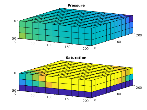
figure(2),
subplot(2,1,2-double(isCompr));
bar(nits,1,'EdgeColor','r','FaceColor',[.6 .6 1]);
axis tight, set(gca,'YLim',[0 10]);
hold on,
plotyy(nan,nan,1:numel(dt),dt/day,@plot, ...
@(x,y) plot(x,y,'-o','MarkerFaceColor',[.6 .6 .6]));
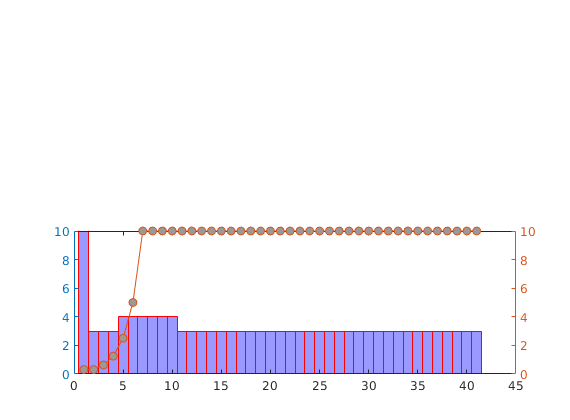
figure(3); hold all
ipr = arrayfun(@(x) x.pressure(inIx), sol)/barsa;
t = arrayfun(@(x) x.time, sol)/day;
fpr = arrayfun(@(x) sum(x.pressure)/G.cells.num, sol)/barsa;
plot(t,ipr,'-', t,fpr, '--');
% chl = get(gca,'Children');
% col=flipud(lines(2));
% for i=1:numel(chl), set(chl(i),'Color',col(ceil(i/2),:),'LineWidth',2); end
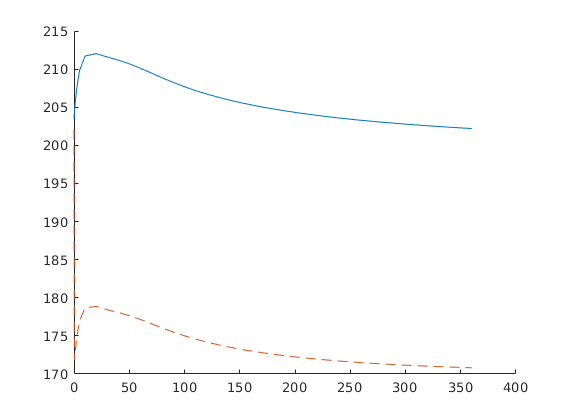
figure(4); hold all
oip = arrayfun(@(x) sum(pv(x.pressure).*(1-x.s).*rhoO(x.pressure)), sol);
plot(t,(ioip - oip)./rhoOS,'-o','MarkerFaceColor',[.6 .6 .6])
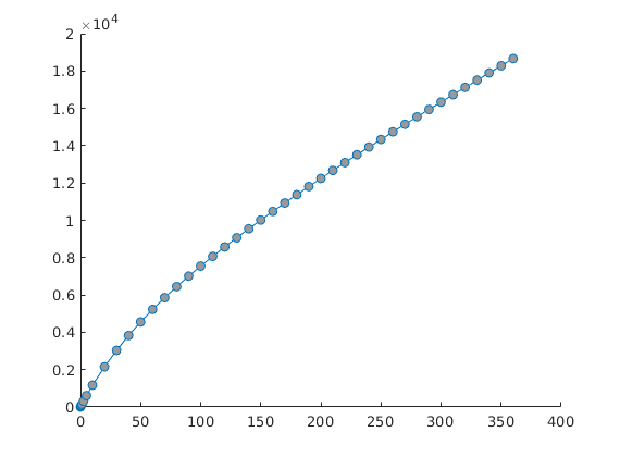
figure(5); hold all
plot(cumsum(isnan(cnd))+1, 1./cnd,'-o');
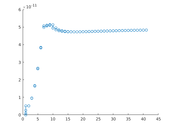
{
g = cartGrid([1 1 1],[Dx Dy Dz]);
figure; colormap(winter);
for i=1:nstep+1
s = sol(i).s;
clf
plotCellData(G,1-s,s>1e-3,'EdgeColor','k','EdgeAlpha',.1);
plotGrid(g,'EdgeColor','k','FaceColor','none');
view(3); plotGrid(G,[inIx; outIx],'FaceColor',[.6 .6 .6]);
view(30,40); caxis([0 1]); axis tight off
axis([-.5 Dx+.5 -.5 Dy+.5 -.5 Dz+.5]);
h=colorbar('horiz');
pos = get(gca,'Position');
set(h,'Position',[.13 .15 .775 .03]); set(gca,'Position',pos);
title(['Time: ' num2str(t(i)) ' days']);
drawnow, pause(.5)
print('-dpng','-r0',sprintf('twoPhaseAD-%02d.png',i-1));
end
function u = outflow(u,~)
end
Advection: classic schemes
Generated from runCases.m
Initial data: set up the initial data and remember to add one ghost cell at each end of the interval. These cells will be used to impose boundary conditions
FontSize = 12; pargs = {'MarkerSize',8};
dx = 1/100;
x = -.5*dx:dx:1+.5*dx;
u0 = sin((x-.1)*pi/.3).^2.*double(x>=.1 & x<=.4);
u0((x<.9) & (x>.6)) = 1;
% Flux function
f = @(u) u;
df = @(u) 0*u + 1;
% Run simulation
uu = upw(u0, .5, dx, 1, f, df, @periodic);
uf = lxf(u0, .5, dx, 1, f, df, @periodic);
uw = lxw(u0, .5, dx, 1, f, df, @periodic);
% Plot results
figure('Position',[293 539 1000 300]);
i = (x>=.1 & x<=.4);
subplot(1,4,1,'FontSize',FontSize)
plot([0 x(i) .6 .6 .9 .9 1], [0 u0(i) 0 1 1 0 0], '-k',...
x(2:end-1), uu(2:end-1), '.', pargs{:});
axis([0 1 -.2 1.2]); title('Upwind');
subplot(1,4,2,'FontSize',FontSize)
plot([0 x(i) .6 .6 .9 .9 1], [0 u0(i) 0 1 1 0 0], '-k',...
x(2:end-1), uf(2:end-1), '.', pargs{:});
axis([0 1 -.2 1.2]); title('Lax-Friedrichs');
subplot(1,4,3,'FontSize',FontSize)
plot([0 x(i) .6 .6 .9 .9 1], [0 u0(i) 0 1 1 0 0], '-k',...
x(2:end-1), uw(2:end-1), '.', pargs{:});
axis([0 1 -.2 1.2]); title('Lax-Wendroff');
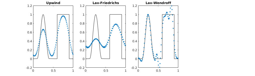
Advection: high-resolution schemes
lim = @(r) max(0,min(2*r,min(.5+.5*r,2)));
xh = -1.5*dx:dx:1+1.5*dx;
u0 = sin((xh-.1)*pi/.3).^2.*double(xh>=.1 & xh<=.4);
u0((xh<.9) & (xh>.6)) = 1;
un = nt (u0, .25, dx, 1, f, df, @periodic, lim);
%uc = cuw(u0, .25, dx, 1, f, df, @periodic, lim);
subplot(1,4,4,'FontSize',FontSize)
i = (xh>=.1 & xh<=.4);
plot([0 x(i) .6 .6 .9 .9 1], [0 u0(i) 0 1 1 0 0], '-k', ...
xh(3:end-2), un(3:end-2), '.', pargs{:});
title('Nessyahu-Tadmor');
axis([0 1 -.2 1.2]);
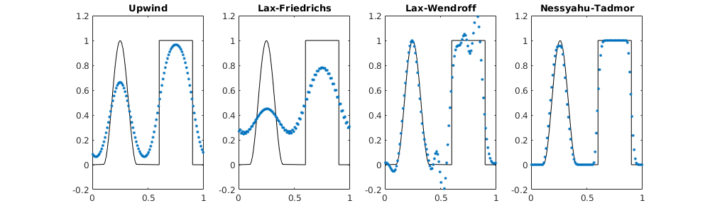
Burgers’ equation
f = @(u) .5*u.^2;
df = @(u) u;
% Run simulations
dx = 1/20;
x = -1-0.5*dx:dx:1+0.5*dx;
uf = sin(2*pi*x).*double(x>=-.5 & x<=.5);
uw = lxw (uf, .995, dx, .6, f, df, @outflow);
uf = lxf (uf, .995, dx, .6, f, df, @outflow);
xh = -1-1.5*dx:dx:1+1.5*dx;
uh = sin(2*pi*xh).*double(xh>=-.5 & xh<=.5);
uh = nt(uh, .495, dx, .6, f, df, @outflow, lim);
dx = 1/1000;
xr = -1-1.5*dx:dx:1+1.5*dx;
ur = sin(2*pi*xr).*double(xr>=-.5 & xr<=.5);
ur = cuw(ur, .495, dx, .6, f, df, @outflow);
% Plot results
figure('Position',[293 539 1000 300]);
subplot(1,3,1)
plot(xr(3:end-2),ur(3:end-2), '-', x(2:end-1), uf(2:end-1), 'o');
axis([-1 1 -1.1 1.1]); title('Lax--Friedrichs');
subplot(1,3,2)
plot(xr(3:end-2),ur(3:end-2), '-', x(2:end-1), uw(2:end-1), 'o');
axis([-1 1 -1.1 1.1]); title('Lax-Wendroff');
subplot(1,3,3)
plot(xr(3:end-2),ur(3:end-2), '-', xh(3:end-2), uh(3:end-2), 'o');
axis([-1 1 -1.1 1.1]); title('Nessyahu-Tadmor');
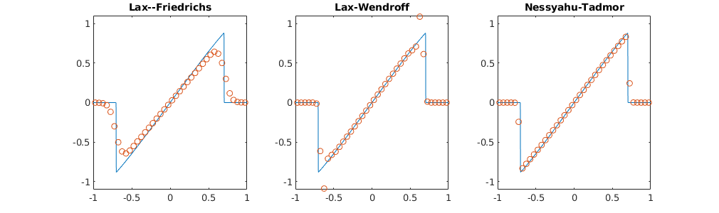
Buckley-Leverett problem: classical schemes vs high-resolution
Flux function
f = @(u) u.^2./(u.^2 + (1-u).^2);
s = linspace(0,1,501);
dfv = max(diff(f(s))./diff(s));
df = @(u) 0*u + dfv;
% reference solution
T = 0.65;
dx = 1/1000;
xr = -.5*dx:dx:1+.5*dx;
u0 = 0*xr; u0(xr<.1)=1.0;
ur = upw(u0, .995, dx, T, f, df, @outflow);
% Solutions on coarser grids
N = 50;
dx = 1/N;
x = -.5*dx:dx:1+.5*dx;
u0 = 0*x; u0(x<.1)=1.0;
figure('Position',[293 539 1000 300]);
subplot(1,4,1,'FontSize',FontSize)
uu = upw(u0, .995, dx, T, f, df, @outflow);
plot(xr(2:end-1),ur(2:end-1), '-k', x(2:end-1), uu(2:end-1), '.', pargs{:});
axis([0 1 -.05 1.05]); title('Upwind');
subplot(1,4,2,'FontSize',FontSize)
uf = lxf(u0, .995, dx, T, f, df, @outflow);
plot(xr(2:end-1),ur(2:end-1), '-k', x(2:end-1), uf(2:end-1), '.', pargs{:});
axis([0 1 -.05 1.05]); title('Lax-Friedrichs');
subplot(1,4,3,'FontSize',FontSize)
uw = lxw(u0, .995, dx, T, f, df, @outflow);
plot(xr(2:end-1),ur(2:end-1), '-k', x(2:end-1), uw(2:end-1), '.', pargs{:});
axis([0 1 -.05 1.05]); title('Lax-Wendroff');
% High-resolution schemes
xh = -1.5*dx:dx:1+1.5*dx;
u0 = 0*xh; u0(xh<.1)=1.0;
un = nt(u0, .495, dx, T, f, df, @inflow);
uc = cuw(u0, .495, dx, T, f, df, @inflow);
subplot(1,4,4,'FontSize',FontSize)
plot(xh(3:end-2), un(3:end-2), '.', xh(3:end-2), uc(3:end-2), '.r', ...
xr(2:end-1),ur(2:end-1), 'k-', pargs{:});
axis([0 1 -.05 1.05]); title('High-resolution');
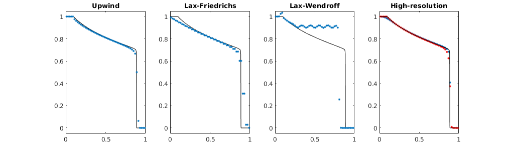
Buckley-Leverett problem: using ‘incomp’ module
mrstModule add incomp
G = computeGeometry(cartGrid([100,1],[1 1]));
rock = makeRock(G, ones(G.cells.num,1), ones(G.cells.num,1));
fluid = initSimpleFluid('mu' , [ 1, 1] .* centi*poise , ...
'rho', [1000, 1000] .* kilogram/meter^3, ...
'n' , [ 2, 2]);
bc = fluxside([], G, 'Left', 1, 'sat', [1 0]);
bc = fluxside(bc, G, 'Right', -1, 'sat', [0 1]);
hT = computeTrans(G, rock);
rSol = initState(G, [], 0, [0 1]);
rSol = incompTPFA(rSol, G, hT, fluid, 'bc', bc);
rSole = explicitTransport(rSol, G, .65, rock, fluid, 'bc', bc);
rSoli = rSol; n = 13;
for i=1:n
rSoli = implicitTransport(rSoli, G, .65/n, rock, fluid, 'bc', bc);
end
rSolt = rSol; n = 130;
for i=1:n
rSolt = implicitTransport(rSolt, G, .65/n, rock, fluid, 'bc', bc);
end
dx = 1/1000;
xr = -.5*dx:dx:1+.5*dx;
u0 = 0*xr; u0(1)=1.0;
ur = upw(u0, .995, dx, .65, f, df, @outflow);
figure;
plot(G.cells.centroids(:,1), rSole.s(:,1),'o', ...
G.cells.centroids(:,1), rSolt.s(:,1), 's', ...
G.cells.centroids(:,1), rSoli.s(:,1), '*', ...
xr(2:end-1),ur(2:end-1),'-k');
legend('Explicit','Implicit, CFL=1','Implicit, CFL=10','Location','SouthWest');
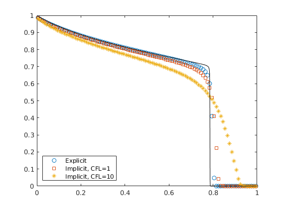
function u=upw(u0,cfl,dx,T,flux,df,boundary)
u = u0; t = 0.0;
dt = cfl*dx/max(abs(df(u0)));
i = 2:numel(u0)-1;
while (t<T)
if (t+dt > T)
dt = (T-t);
end
t=t+dt;
u = boundary(u);
f = flux(u);
u(i) = u(i) - dt/dx*(f(i)-f(i-1));
dt = cfl*dx/max(abs(df(u)));
end
Visualizing the Johansen Data Set
Generated from showJohansenNPD.m
The Johansen formation is a candidate site for large-scale CO2 storage offshore the south-west coast of Norway. The MatMoRA project has developed a set of geological models based on available seismic and well data. Herein, we will inspect one instance of the model in more detail.
Faults and active/inactive cells
We start by reading the model from a file in the Eclipse format (GRDECL), picking the sector model with five vertical layers in the Johansen formation and with five shale layers above and one below.
sector = fullfile(getDatasetPath('johansen'), 'NPD5');
filename = [sector, '.grdecl'];
G = processGRDECL(readGRDECL(filename));
Porosity
The porosity data are given with one value for each cell in the model. We read all values and then pick only the values corresponding to active cells in the model.
args = {'EdgeAlpha'; 0.1; 'EdgeColor'; 'k'};
p = load([sector, '_Porosity.txt'])'; p = p(G.cells.indexMap);
h = plotCellData(G, p, args{:}); view(-45,15),
axis tight off, zoom(1.15), caxis([0.1 0.3]), colorbar;
set(gca,'Clipping','off')
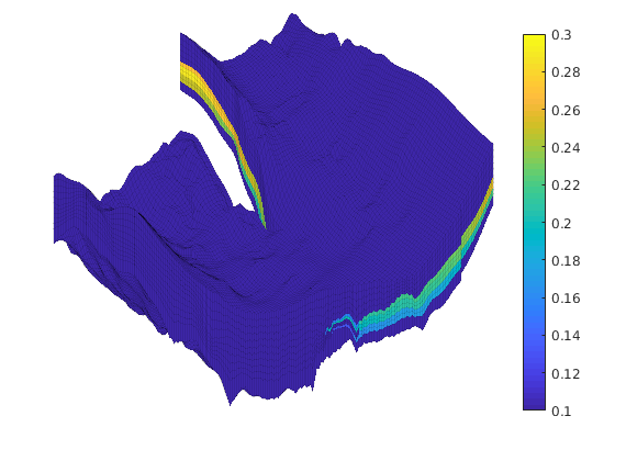
From the plot, it seems like the formation has been pinched out and only contains the shale layers in the front part of the model. We verify this by plotting a filtered porosity field in which all values smaller than or equal 0.1 have been taken out.
delete(h), view(-15,40)
plotGrid(G,'FaceColor','none', args{:});
plotCellData(G, p, find(p>0.1), args{:})
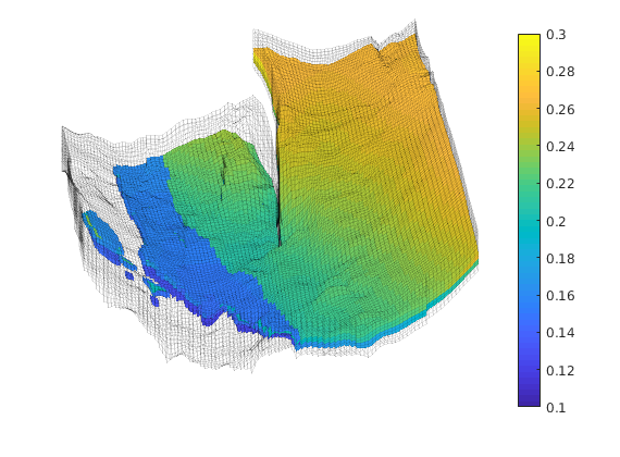
Permeability
The permeability is given as a scalar field (Kx) similarly as the porosity. The tensor is given as K = diag(Kx, Kx, 0.1Kx) and we therefore only plot the x-component, Kx, using a logarithmic color scale.
clf
K = load([sector '_Permeability.txt'])'; K=K(G.cells.indexMap);
plotCellData(G, log10(K), args{:});
view(-45,15), axis tight off, zoom(1.15)
set(gca,'Clipping','off')
[hc,hh] = colorbarHist(K, [0.001 1000], 'East', 100, true);
p = get(hh,'Position'); set(hh,'Position',p.*[1 1 1.5 1]);
set(get(hh,'Children'),'FaceColor',[.6 .6 .6]);
set(hc,'Fontsize',16,'FontWeight','bold', 'XTick', 0.5, 'XTickLabel','mD', ...
'YTickLabel', {10.^(-3:3)});
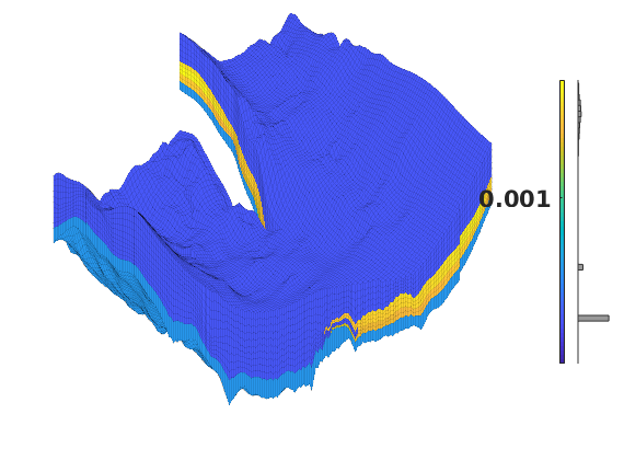
To show more of the permeability structure, we strip away the shale layers, starting with the layers with lowest permeability on top.
clf,
plotGrid(G,'FaceColor','none',args{:});
plotCellData(G, log10(K), find(K>0.01), args{:});
view(-60,40), axis tight off, zoom(1.15)
set(gca,'Clipping','off')
[hc,hh] = colorbarHist(K(K>0.01), [0.01 1000], 'East', 100, true);
set(get(hh,'Children'),'FaceColor',[.6 .6 .6]);
set(hc,'Fontsize',16,'FontWeight','bold', 'XTick', 0.5, 'XTickLabel','mD', ...
'YTickLabel', {10.^(-2:3)});
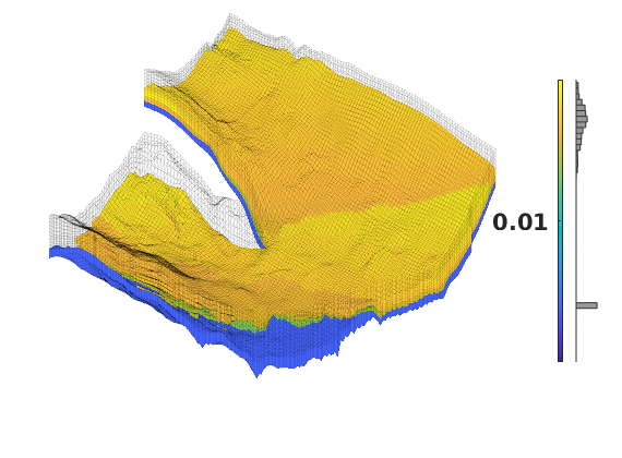
Then we also take away the lower shale layer and plot the permeability using a linear color scale.
lf; plotGrid(G,'FaceColor','none',args{:});
h = plotCellData(G, K, find(K>0.1), args{:});
view(-60,40), axis tight off, zoom(1.15)
set(gca,'Clipping','off')
[hc,hh] = colorbarHist(K(K>0.1), [0 900], 'East', 100, false);
set(get(hh,'Children'),'FaceColor',[.6 .6 .6]);
set(hc,'Fontsize',16,'FontWeight','bold', 'XTick', 0.5, 'XTickLabel','mD');
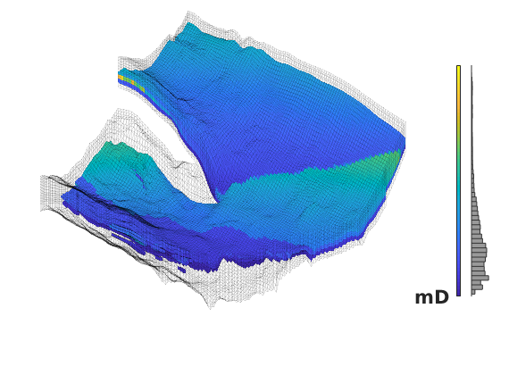
Visualizing a realization of the SAIGUP project
Generated from showRockSAIGUP.m
The <http://www.fault-analysis-group.ucd.ie/Projects/SAIGUP.html>SAIGUP project is a systematic assessment of uncertainty in reserves and production estimates within an objectively defined geological parameterisation encompassing the majority of European clastic oil reservoirs. A broad suite of shallow marine sedimentological reservoir types are indexed to continuously varying 3D anisotropy and heterogeneity levels. Structural complexity ranges from unfaulted to compartmentalised, and fault types from transmissive to sealing. Several geostatistical realisations each for the geologically diverse reservoir types covering the pre-defined parameter-space are up-scaled, faulted and simulated with an appropriate production strategy for an approximately 20 year period. Herein, we will inspect in detail one instance of the model, which can be downloaded from the <http://www.sintef.no/Projectweb/MRST>MRST webpage
Show the structural model
We start by reading the model from a file in the Eclipse format (GRDECL), The file contains both active and inactive cells
grdecl = fullfile(getDatasetPath('SAIGUP'), 'SAIGUP.GRDECL');
grdecl = readGRDECL(grdecl);
MRST uses the strict SI conventions in all of its internal caluclations. The SAIGUP model, however, is provided using the ECLIPSE ‘METRIC’ conventions (permeabilities in mD and so on). We use the functions getUnitSystem and convertInputUnits to assist in converting the input data to MRST’s internal unit conventions.
usys = getUnitSystem('METRIC');
grdecl = convertInputUnits(grdecl, usys);
Define geometry and rock properties
We generate a space-filling geometry using the processGRDECL function and then compute a few geometric primitives (cell volumes, centroids, etc.) by means of the computeGeometry function.
G = processGRDECL(grdecl);
G = computeGeometry(G);
figure
args = {'EdgeAlpha'; 0.1; 'EdgeColor'; 'k'};
plotGrid(G,'FaceColor','none', args{:});
plotFaces(G,find(G.faces.tag>0),'FaceColor','r', args{:});
axis tight off; set(gca,'DataAspect',[1 1 0.1]);
view(-65,60); zoom(1.1); camdolly(0,-0.2,0)
set(gca,'Clipping','off')
% The media (rock) properties can be extracted by means of the
% <matlab:doc('grdecl2Rock') grdecl2Rock> function.
rock = grdecl2Rock(grdecl, G.cells.indexMap);
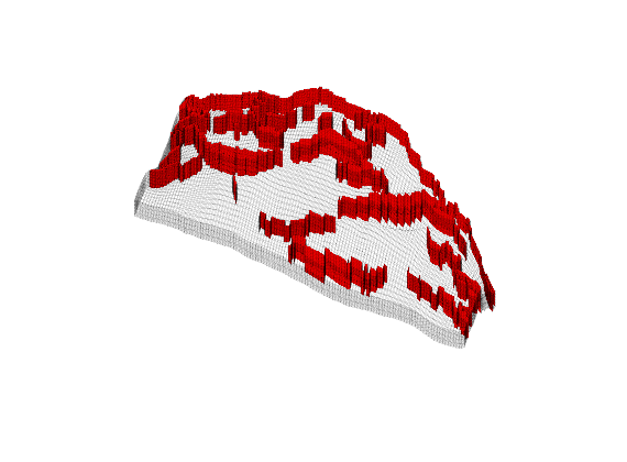
Porosity
The porosity data are given with one value for each cell in the model. First, we show the porosities as they are generated on a Cartesian grid that corresponds to geological ‘time zero’, i.e., an imaginary time at which all the depositional layers were stacked as horizontally on a Cartesian grid.
p = reshape(grdecl.PORO, G.cartDims);
clf
slice(p, 1, 1, 1); view(-135,30), shading flat,
axis equal off, set(gca,'ydir','reverse','zdir','reverse')
colorbar('horiz'); caxis([0.01 0.3]);
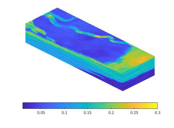
Likewise, we show a histogram of the porosity
hist(p(:),100);
h=get(gca,'Children');
set(h(1),'EdgeColor',[0 0 0.4],'FaceColor','none')
h = legend('Porosity'); set(h,'FontSize',16);
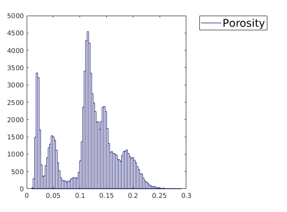
Then we show the porosities mapped onto the structural grid
clf
plotCellData(G,rock.poro, args{:});
axis tight off; set(gca,'DataAspect',[1 1 0.1]);
view(-65,55); zoom(1.4); camdolly(0,-0.2,0)
set(gca,'Clipping','off')
colorbar('horiz'); caxis([0.1 0.3])
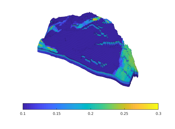
show also the net-to-gross
clf
plotCellData(G,rock.ntg, args{:});
axis tight off; set(gca,'DataAspect',[1 1 0.1]);
view(-65,60); zoom(1.4); camdolly(0,-0.2,0)
set(gca,'Clipping','off')
colorbar('horiz'); %caxis([0.1 0.3])
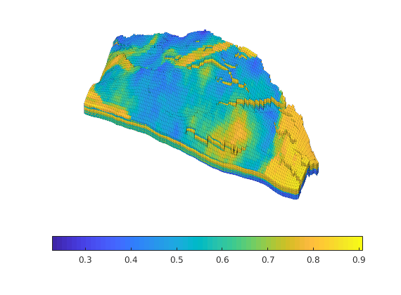
and the satnum
clf
SN = grdecl.SATNUM(G.cells.indexMap); j = jet(60);
plotCellData(G,SN, args{:});
axis tight off; set(gca,'DataAspect',[1 1 0.1]);
view(-65,60); zoom(1.4); camdolly(0,-0.2,0)
set(gca,'Clipping','off')
colorbar('horiz'); caxis([0.5 6.5]), colormap(j(1:10:end,:))
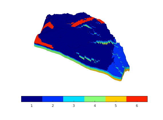
and a plot where we split them up
clf
plotGrid(G,'FaceColor','none', args{:});
axis tight off; set(gca,'DataAspect',[1 1 0.1]);
view(-65,60); zoom(1.4); camdolly(0,-0.2,0)
set(gca,'Clipping','off')
caxis([0.5 6.5]), colormap(j(1:10:end,:))
h1 = plotCellData(G,SN, find(SN==1), args{:});
h2 = plotCellData(G,SN, find(SN==5), args{:});
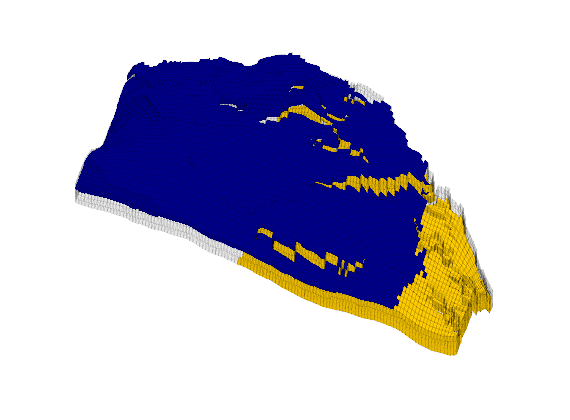
delete([h1,h2])
h1 = plotCellData(G,SN, find(SN==2), args{:});
h2 = plotCellData(G,SN, find(SN==4), args{:});
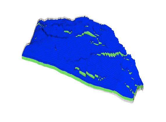
delete([h1,h2])
h1 = plotCellData(G,SN, find(SN==3), args{:});
h2 = plotCellData(G,SN, find(SN==6), args{:});
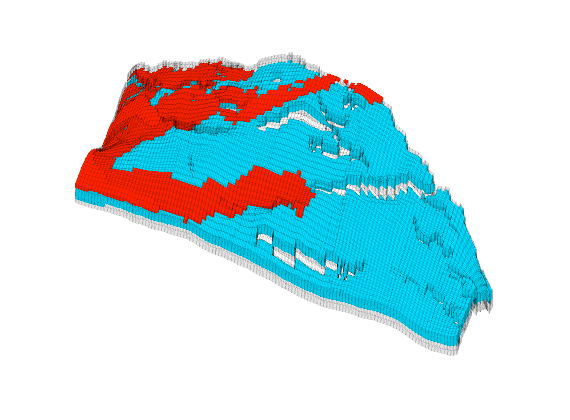
Permeability
The permeability is given as a tridiagonal tensor K = diag(Kx, Ky, Kz) and we therefore plot each of the horizontal and vertical components using a logarithmic color scale.
figure;
h = plotCellData(G,log10(rock.perm(:,1)), args{:});
axis tight off; set(gca,'DataAspect',[1 1 0.1]);
view(-65,55); zoom(1.4); camdolly(0,-0.2,0)
set(gca,'Clipping','off')
% Manipulate the colorbar to get the ticks we want
hc = colorbar('horiz');
cs = [0.001 0.01 0.1 1 10 100 1000 10000];
caxis(log10([min(cs) max(cs)]*milli*darcy));
set(hc, 'YTick', 0.5, 'YTickLabel','mD', ...
'XTick', log10(cs*milli*darcy), 'XTickLabel', num2str(cs'));
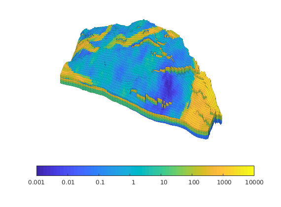
Vertical permeability
delete(h)
plotCellData(G,log10(rock.perm(:,3)), args{:});
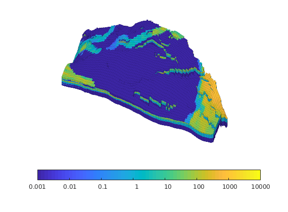
Likewise, we show a histogram of the permeability
clf
Kx = rock.perm(:,1)./(milli*darcy);
Kz = rock.perm(:,3)./(milli*darcy);
hist(log10(Kx),100);
hold on
hist(log10(Kz(Kz>0)),100);
hold off
h=get(gca,'Children');
set(h(1),'EdgeColor',[0 0 0.4],'FaceColor','none')
set(h(2),'EdgeColor',[0.6 0 0],'FaceColor','none')
h = legend('Horizontal','Vertical'); set(h,'FontSize',16);
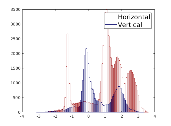
and one histogram per rock type
figure('Position',[0 60 900 350]);
col = jet(60); col=col(1:10:end,:);
for i=1:6
subplot(2,3,i);
hist(log10(Kx(SN==i)), 100);
h = findobj(gca,'Type','patch');
set(h,'FaceColor',col(i,:),'EdgeColor',col(i,:))
set(gca,'XLim',[-3 4],'XTick',-2:2:4,'XTickLabel',num2str(10.^(-2:2:4)'));
end
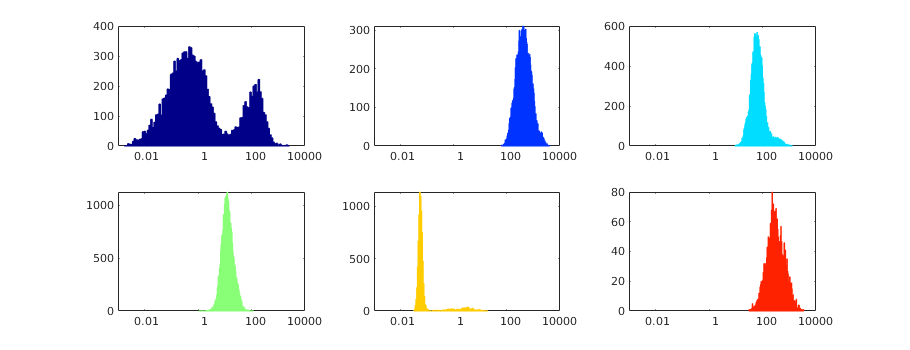
Finally, show the multiplicator values
igure
Mx = grdecl.MULTX(G.cells.indexMap);
My = grdecl.MULTY(G.cells.indexMap);
Mz = grdecl.MULTZ(G.cells.indexMap);
plotGrid(G,'FaceColor','none','EdgeAlpha',0.1);
plotCellData(G,Mz,find(Mz<1),args{:});
axis tight off; set(gca,'DataAspect',[1 1 0.1]);
view(-65,55); zoom(1.4); camdolly(0,-0.2,0)
set(gca,'Clipping','off')
colorbar('horiz');
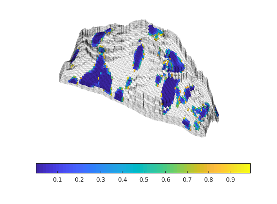
Modle 2 of the 10th SPE Comparative Solution Project
Generated from showSPE10.m
The data set was originally posed as a benchmark for upscaling methods. The 3-D geological model consists of 60x220x85 grid cells, each of size 20ftx10ftx2ft. The model is a geostatistical realization from the Jurassic Upper Brent formations, in which one can find the giant North Sea fields of Statfjord, Gullfaks, Oseberg, and Snorre. In this specific model, the top 70 ft (35 layers) represent the shallow-marine Tarbert formation and the lower 100 ft (50 layers) the fluvial Ness formation. The data can be obtained from the SPE website: http://www.spe.org/web/csp/ The data set is used extensively in the literature, and for this reason, MRST has a special module that will download and provide easy access to the data set. In this example, we will inspect the SPE10 model in more detail.
mrstModule add spe10
doprint = false;
Load the model
The first time you access the model, it will be downloaded from the official websiet of the comparative solution project. Depending upon your internet connection, this may take quite a while, so please be patient.
rock = getSPE10rock();
p = rock.poro;
K = convertTo(rock.perm,milli*darcy);
show p
slice( reshape(p,60,220,85), [1 220], 60, [1 85]);
shading flat, axis equal off, set(gca,'zdir','reverse'), box on;
colorbar('horiz');
set(gcf,'renderer','painters');
if doprint
print -depsc2 rock-spe10-poro.eps; %#ok<UNRCH>
print -dpng rock-spe10-poro.png;
end
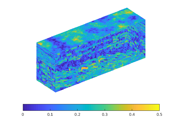
show Kx
slice( reshape(log10(K(:,1)),60,220,85), [1 220], 1, [1 85]);
shading flat, axis equal off, set(gca,'zdir','reverse'), box on;
h=colorbar('horiz');
set(h,'XTickLabel',10.^get(h,'XTick'));
set(h,'YTick',mean(get(h,'YLim')),'YTickLabel','mD');
set(gcf,'renderer','painters');
if doprint
print -depsc2 rock-spe10-Kx.eps; %#ok<UNRCH>
print -dpng rock-spe10-Kx.png;
end
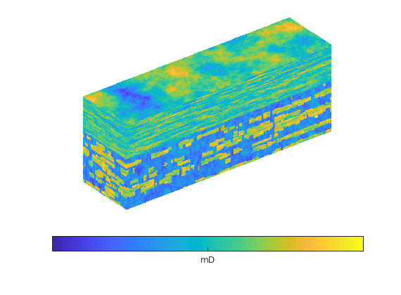
show Ky
slice( reshape(log10(K(:,2)),60,220,85), [1 220], 60, [1 85]);
shading flat, axis equal off, set(gca,'zdir','reverse'), box on;
h=colorbar('horiz');
set(h,'XTickLabel',10.^get(h,'XTick'));
set(h,'YTick',mean(get(h,'YLim')),'YTickLabel','mD');
set(gcf,'renderer','painters');
if doprint
print -depsc2 rock-spe10-Ky.eps; %#ok<UNRCH>
print -dpng rock-spe10-Ky.png;
end
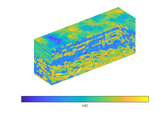
show Kz
slice( reshape(log10(K(:,3)),60,220,85), [1 220], 60, [1 85]);
shading flat, axis equal off, set(gca,'zdir','reverse'), box on;
h=colorbar('horiz');
set(h,'XTickLabel',10.^get(h,'XTick'));
set(h,'YTick',mean(get(h,'YLim')),'YTickLabel','mD');
set(gcf,'renderer','painters');
if doprint
print -depsc2 rock-spe10-Kz.eps; %#ok<UNRCH>
print -dpng rock-spe10-Kz.png;
end
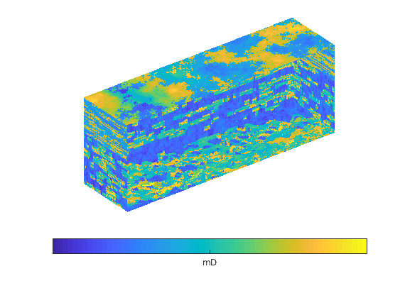
show horizontal permeability distributions
hist(log10(K(220*60*35+1:end,1)),101);
hold on
hist(log10(K(1:220*60*35,1)),101)
hold off
h=get(gca,'Children');
set(h(1),'EdgeColor',[0 0 0.4],'FaceColor','none')
set(h(2),'EdgeColor',[0.7 0 0],'FaceColor','none')
h=legend('Ness','Tarbert'); set(h,'FontSize',16);
if doprint
print -depsc2 rock-spe10-Kx-hist.eps; %#ok<UNRCH>
end
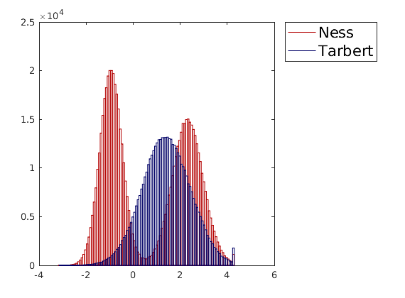
show vertical permeability distributions
clf;
hist(log10(K(1:220*60*35,3)),101)
hold on
hist(log10(K(220*60*35+1:end,3)),101);
hold off
h=get(gca,'Children');
set(h(2),'EdgeColor',[0 0 0.4],'FaceColor','none')
set(h(1),'EdgeColor',[0.7 0 0],'FaceColor','none')
h=legend('Tarbert','Ness');set(h,'FontSize',16);
if doprint
print -depsc2 rock-spe10-Kz-hist.eps; %#ok<UNRCH>
end
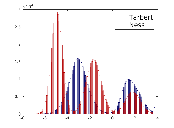
show porosity distributions
T = p(1:220*60*35); pN = p(220*60*35+1:end);
pb = linspace(0,0.5,101);
N=histc(pN,pb); bar(pb,N,'histc');
hold on
N=histc(pT,pb); bar(pb,N,'histc');
hold off;
h=get(gca,'Children');
set(h(1),'EdgeColor',[0 0 0.4],'FaceColor','none')
set(h(2),'EdgeColor',[0.7 0 0],'FaceColor','none')
h=legend('Ness','Tarbert');set(h,'FontSize',16);
set(gca,'XLim',[0 0.5]);
if doprint
print -depsc2 rock-spe10-poro-hist.eps; %#ok<UNRCH>
end
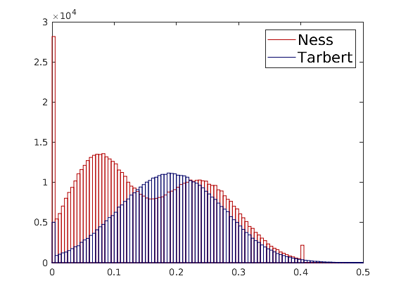
Simple examples
Generated from simpleRockExamples.m
In this example we will go through a set of elementary examples that demonstrate how to generate petrophysical properties in MRST
Homogeneous, isotropic properties
G = cartGrid([1000 100]);
rock = makeRock(G, 200*milli*darcy,.2);
plotCellData(G, rock.poro,'EdgeColor','w');
Homogeneous, anisotropic properties
rock.perm = repmat( [100 100 10].*milli*darcy, [G.cells.num,1]);
clf
plotCellData(G, rock.perm./max(rock.perm(:)), 'edgeColor', 'w');

Carman-Kozeny
First in 2D
G = cartGrid([50 20]);
p = gaussianField(G.cartDims, [0.2 0.4], [11 3], 2.5);
K = p.^3.*(1e-5)^2./(0.81*72*(1-p).^2);
rock = makeRock(G, K(:), p(:));
clf
plotCellData(G,rock.poro);
colorbar('horiz'); axis equal tight;
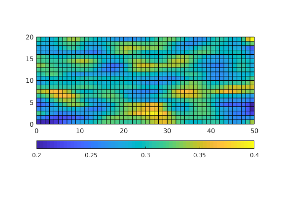
Then in 3D
G = cartGrid([50 20 10]);
p = gaussianField(G.cartDims, [0.2 0.4], [5 3 1], 2.5);
K = p.^3.*(1e-5)^2./(0.81*72*(1-p).^2);
rock = makeRock(G, K(:), p(:));
clf
plotCellData(G,convertTo(rock.perm,milli*darcy));
colorbar('horiz'); axis equal tight; view(3);
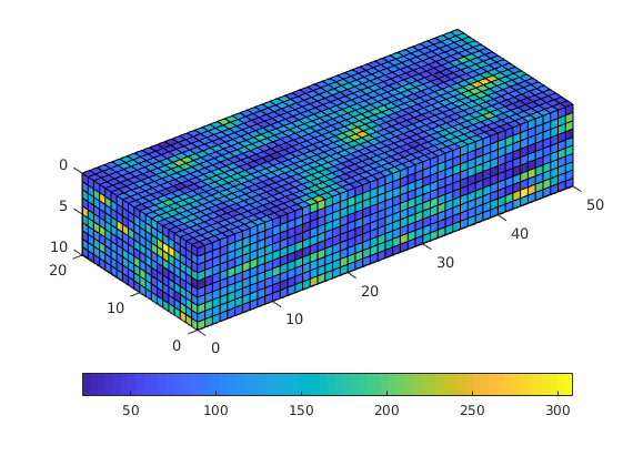
Lognormal, layered in 3D
= processGRDECL(simpleGrdecl([50 30 10], 0.12));
K = logNormLayers(G.cartDims, [100 400 50 350], ...
'indices', [1 2 5 7 11]);
clf
plotCellData(G,log10(K),'EdgeColor','k'); view(45,30);
axis tight off, set(gca,'DataAspect',[0.5 1 1])
h=colorbar('horiz'); ticks=25*2.^(0:5);
set(h,'XTick',log10(ticks),'XTickLabel',ticks);
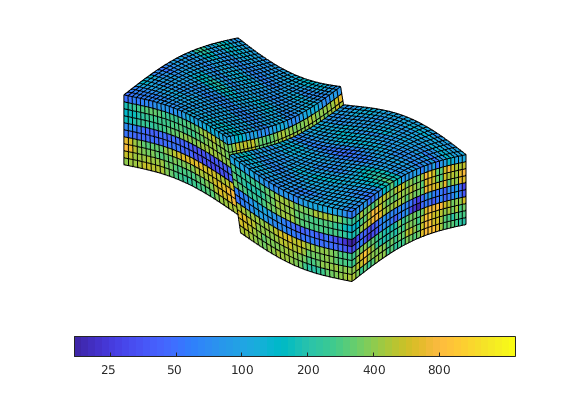
Averaging of SPE10 layer
Generated from averagingExample1.m
To illustrate the implementation of various types of averaging techniques, we consider a single layer of the SPE10 model and compare the effective permeabilities obtained by arithmetic, harmonic, and harmonic-arithmetic averaging.
mrstModule add spe10 coarsegrid;
Setup model
fine = [40 60];
G = cartGrid(fine, fine);
G = computeGeometry(G);
rock = getSPE10rock(1:fine(1),1:fine(2),46);
rock.perm = rock.perm(:,1:2);
% The coarse grid
coarse = [10 15];
q = partitionUI(G,coarse);
cG = cartGrid(coarse,fine);
Compute the averages
The arithmetic and harmonic averages are straightforward. To compute the harmonic-arithmetic average, we temporary partition that coincides with the coarse grid in along the given axial direction and with the original fine grid in the other directions. Then we map the averaged values back onto the fine grid and perform a standard arithmetic averaging.
clear crock*
vol = G.cells.volumes;
for i=1:size(rock.perm,2)
crock1.perm(:,i) = accumarray(q,vol.*rock.perm(:,i))./accumarray(q,vol);
crock2.perm(:,i) = accumarray(q,vol)./accumarray(q,vol./rock.perm(:,i));
dims = G.cartDims; dims(i)=coarse(i);
qq = partitionUI(G, dims);
K = accumarray(qq,vol)./accumarray(qq,vol./rock.perm(:,i));
crock3.perm(:,i) = accumarray(q,K(qq).*vol)./accumarray(q,vol);
end
Plot the resulting effective permeabilities
To improve the visualization we enhance the colorbar by adding a small histogram of permeability values
px = log10([min(rock.perm(:,1)) max(rock.perm(:,1))]);
clf, set(gcf,'Position',[500 400 880 410]);
subplot(1,4,1);
plotCellData(G,log10(rock.perm(:,2)),'EdgeColor','none');
plotGrid(cG,'FaceColor','none','EdgeColor','k'); caxis(px); axis tight off
title('Fine scale');
subplot(1,4,2);
plotCellData(cG,log10(crock1.perm(:,2)),'EdgeColor','k');
caxis(px); axis tight off
title('Arithmetic');
subplot(1,4,3);
plotCellData(cG,log10(crock2.perm(:,2)),'EdgeColor','k');
caxis(px); axis tight off
title('Harmonic');
subplot(1,4,4);
plotCellData(cG,log10(crock3.perm(:,2)),'EdgeColor','k');
caxis(px); axis tight off
title('Harmonic-arithmetic');
perm{1} = log10(rock.perm(:,2));
perm{2} = log10(crock1.perm(:,2));
perm{3} = log10(crock2.perm(:,2));
perm{4} = log10(crock3.perm(:,2));
for i=1:4
subplot(1,4,i);
[h,ax] = colorbarHist(perm{i},[-18 -10],'South');
set(h,'XTick',-16:2:-12,'XTickLabel',{'.1', '10', '1000'});
end
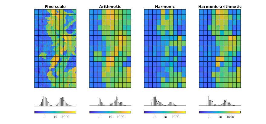
Assessment of upscaling accuracy on 8x8x8 grid
Generated from averagingExample2.m
We upscale a small 8x8x8 cube with three different permeability realizations and measure the ratio between the outflows computed on the upscaled and the original fine-scale model.
mrstModule add coarsegrid incomp spe10 upscaling
Setup case
G = computeGeometry(cartGrid([8 8 8]));
coarse = [1 1 1];
cG = computeGeometry(cartGrid(coarse,G.cartDims));
fluid = initSingleFluid('mu' , 1*centi*poise , ...
'rho', 1014*kilogram/meter^3);
fl = {'East', 'North', 'Top'};
fr = {'West', 'South', 'Bottom'};
clc, clf, set(gcf,'Position',[500 400 800 300]);
disp(' Arithmetic Harmonic Harm-arith');
for n=1:3
disp('-----------------------------------------------------------------');
switch n
case 1
K = repmat([50 150 400 300 10 250 100 350], ...
prod(G.cartDims(1:2)),1);
rock.perm = K(:)*[1 1 1]*milli*darcy;
disp('Layered:');
case 2
disp('Tarbert');
rock = getSPE10rock(9:16,9:16,3:10);
case 3
disp('Upper Ness');
rock = getSPE10rock(9:16,9:16,43:50);
end
subplot(1,3,n);
plotCellData(G,log10(rock.perm(:,1)/(milli*darcy))); view(3); axis off; zoom(1.3);
set(gca,'Clipping','off')
-----------------------------------------------------------------
Layered:
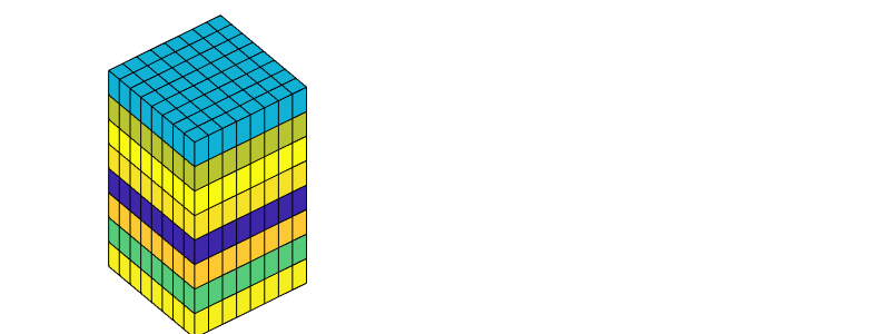
-----------------------------------------------------------------
Tarbert
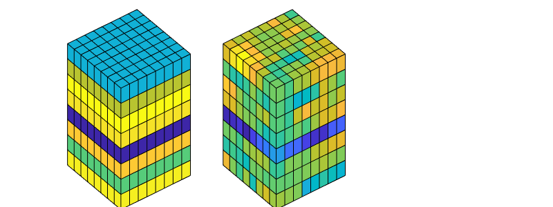
-----------------------------------------------------------------
Upper Ness
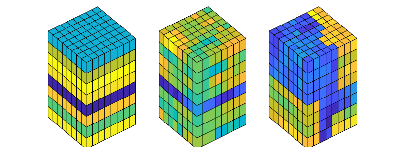
Upscale values
q = ones(G.cells.num,1);
vol = G.cells.volumes;
crock = cell(3,1);
for i=1:size(rock.perm,2)
% Arithmetic
crock{1}.perm(:,i) = accumarray(q,vol.*rock.perm(:,i)) ./ ...
accumarray(q,vol);
% Harmonic
crock{2}.perm(:,i) = accumarray(q,vol) ./ ...
accumarray(q,vol./rock.perm(:,i));
% Harmonic-arithmetic
dims = G.cartDims; dims(i)=coarse(i);
qq = partitionUI(G, dims);
K = accumarray(qq,vol)./accumarray(qq,vol./rock.perm(:,i));
crock{3}.perm(:,i) = accumarray(q,K(qq).*vol)./accumarray(q,vol);
end
Compare upscaling
for j=1:numel(fl)
% Fine-scale problem
bc = pside([], G, fl{j}, barsa);
faces = bc.face;
bc = pside(bc, G, fr{j}, 0);
hT = computeTrans(G, rock);
xr = incompTPFA(initResSol(G,0), G, hT, fluid, 'bc', bc);
flux = sum(xr.flux(faces));
fprintf(' %5s -> %6s: ', fl{j}, fr{j});
for i=1:3
cbc = pside([], cG, fl{j}, barsa);
cfaces = cbc.face;
cbc = pside(cbc, cG, fr{j}, 0);
chT = computeTrans(cG, crock{i});
x = incompTPFA(initResSol(cG,0), cG, chT, fluid, 'bc', cbc);
fprintf('\t%f', x.flux(cfaces) / flux);
end
fprintf('\n');
end
East -> West: 1.000000 0.266151 1.000000
North -> South: 1.000000 0.266151 1.000000
Top -> Bottom: 3.757266 1.000000 1.000000
East -> West: 1.659138 0.024628 0.852037
North -> South: 1.633738 0.024250 0.852491
Top -> Bottom: 47428.068405 0.323872 0.858847
East -> West: 3.406023 0.000850 0.830259
North -> South: 1.953673 0.000487 0.712832
Top -> Bottom: 6776.849373 0.001990 0.339976
end
disp('-----------------------------------------------------------------');
cax = caxis;
for i=1:3, subplot(1,3,i), caxis(cax); end
h = colorbar;
set(h,'Position',[0.94 0.1100 0.02 0.8150], ...
'XTick', .5, 'XTickLabel','[mD]', ...
'YTickLabel',num2str(10.^(-2:3)'));
Arithmetic Harmonic Harm-arith
-----------------------------------------------------------------
Figures for conceptual illustration of upscaling
Generated from illustrateUpscaling.m
We generate a grid that consists of two facies and then perform an upscaling so that 5x5x5 fine cells are replaced by a coarse block. We show the following four plots: fine grid with one coarse cell, porosity inside this coarse cell, the porosity inside the coarse block, and the coarse model
mrstModule add coarsegrid upscaling
Fine model
G = computeGeometry(cartGrid([40 20 15]));
K1 = gaussianField(G.cartDims, [300 2000]);
p1 = K1(:)*1e-4 + .2;
K2 = gaussianField(G.cartDims, [10 900]);
p2 = K2(:)*1e-4 + .2;
rad1 = G.cells.centroids(:,1).^2 + .5*G.cells.centroids(:,2).^2 ...
+ (G.cells.centroids(:,3)-2).^2;
rad2 = .5*(G.cells.centroids(:,1)-40).^2 + 2*G.cells.centroids(:,2).^2 ...
+ 2*(G.cells.centroids(:,3)-2).^2;
ind = ((rad1>600) & (rad1<1500)) | ((rad2>700) & (rad2<1400));
rock.poro = p2(:);
rock.poro(ind) = p1(ind);
% Plot fine model
figure('Position', [680 280 560 540]);
plotCellData(G,rock.poro,'EdgeColor','k','edgealpha',.1);
view(3); axis tight off
[hc,hh]=colorbarHist(rock.poro,[.2 .4],'South', 80);
pos=get(hc,'Position'); set(hc,'Position',pos - [.02 0 .2 -.01],'FontSize',12);
pos=get(hh,'Position'); set(hh,'Position',pos - [.02 0.02 .2 -.01]);
set(gca,'Position',[.13 .2 .775 .775])
% Generate and plot coarse grid block
p = partitionCartGrid(G.cartDims, G.cartDims/5);
CG = generateCoarseGrid(G, p);
crock.poro = accumarray(p, rock.poro)./accumarray(p,1);
plotGrid(CG,1,'FaceColor','none','EdgeColor','k','LineWidth',1.5);
set(gcf,'PaperPositionMode','auto');
% print -dpng illUpscaling-fine.png;
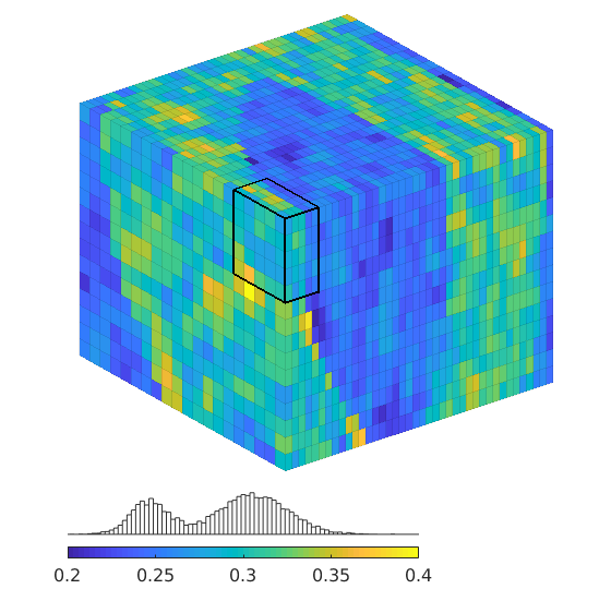
Plot cells inside a single block
figure;
plotCellData(G,rock.poro, p==1, 'EdgeColor','k');
view(3); axis equal off; caxis([0.2 0.4]);
% print -dpng illUpscaling-cells.png;
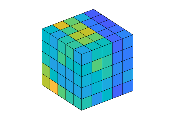
Plot the corresponding coarse block
figure;
cG = computeGeometry(cartGrid(G.cartDims/5,G.cartDims));
plotCellData(cG,crock.poro,1,'EdgeColor','k','LineWidth',1.5);
view(3); axis equal off; caxis([0.2 0.4]);
% print -dpng illUpscaling-block.png;
Coarse model
figure('Position', [680 280 560 540]);
plotCellData(cG,crock.poro,'EdgeColor','k','edgealpha',.1);
view(3); axis tight off
% Generate and plot coarse grid block
plotGrid(CG,1,'FaceColor','none','EdgeColor','k','LineWidth',1.5);
[hc,hh]=colorbarHist(crock.poro,[.2 .4],'South', 40);
pos=get(hc,'Position'); set(hc,'Position',pos + [.2 0 -.2 .01],'FontSize',12);
pos=get(hh,'Position'); set(hh,'Position',pos + [.2 -.025 -.2 .01]);
set(gca,'Position',[.13 .2 .775 .775])
set(gcf,'PaperPositionMode','auto');
% print -dpng illUpscaling-coarse.png;
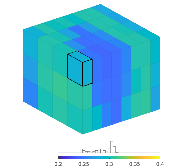
Upscale a problem with a diagonal trend
Generated from permeabilityExample1.m
In this example we will upscale a problem with diagonal trend and compare the results obtained with a flow-based method with pressure-drop and periodic boundary conditions
mrstModule add incomp upscaling;
Set up model
[Lx,Ly] = deal(10);
[nx,ny] = deal(20);
G = computeGeometry(cartGrid([nx ny], [Lx Ly]));
permX = 30*milli*darcy;
[i, j] = gridLogicalIndices(G);
poro = 0.3;
rock.perm = repmat(30*milli*darcy, [G.cells.num, 1]);
rock.poro = repmat(.3, [G.cells.num, 1]);
rock.perm( sin(2*sum(G.cells.centroids(:,:),2)*pi/Lx)>0 ) = 10*milli*darcy;
hT = computeTrans(G, rock);
fluid = initSingleFluid('mu' ,1, 'rho', 1);
clf, plotCellData(G,rock.perm/(milli*darcy),'EdgeColor','none'); colorbar
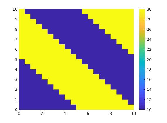
Structures with boundary conditions
d = G.griddim;
[bcl,bcr, Dp]=deal(cell(d,1));
bcsides = {'XMin', 'XMax'; 'YMin', 'YMax'; 'ZMin', 'ZMax'};
for j = 1:d;
bcl{j} = pside([], G, bcsides{j, 1}, 0);
bcr{j} = pside([], G, bcsides{j, 2}, 0);
Dp{j} = 0;
end
Dp{1} = 4*barsa;
L = max(G.faces.centroids)-min(G.faces.centroids);
Pressure-drop boundary conditions
[v,dp] = deal(zeros(d, 1));
for i=1:d
bc = addBC([], bcl{i}.face, 'pressure', Dp{1});
bc = addBC(bc, bcr{i}.face, 'pressure', Dp{2});
xr = initResSol(G, 100*barsa, 1);
xr = incompTPFA(xr, G, hT, fluid, 'bc', bc);
v(i) = sum(xr.flux(bcr{i}.face)) / ...
sum(G.faces.areas(bcr{i}.face));
dp(i) = Dp{1}/L(i);
end
K = convertTo(v./dp, milli*darcy) %#ok<NASGU,NOPTS>
K =
17.2295
17.2295
Periodic boundary conditions
[Gp, bcp] = makePeriodicGridMulti3d(G, bcl, bcr, Dp);
ofaces = cell(d,1);
for j=1:d, ofaces{j} = bcp.face(bcp.tags==j); end
v = nan(d);
dp = Dp{1}*eye(d);
nbcp = bcp;
for i=1:d
for j=1:d, nbcp.value(bcp.tags==j) = dp(j,i); end
xr = initResSol(Gp, 100*barsa, 1);
xr = incompTPFA(xr, Gp, hT, fluid, 'bcp', nbcp);
for j=1:d
v(j,i) = sum(xr.flux(ofaces{j})) / ...
*bcp.sign(bcp.tags==j)) / ...
sum(Gp.faces.areas(ofaces{j}));
end
end
dp = bsxfun(@rdivide, dp, L);
K = convertTo(v/dp, milli*darcy) %#ok<NOPTS>
[V,D] = eig(K) %#ok<NOPTS>
Warning: Face pressures are not well defined for periodic boundary faces
Warning: Face pressures are not well defined for periodic boundary faces
K =
17.2500 -2.2500
-2.2500 17.2500
...
Assessment of upscaling accuracy on 8x8x8 grid
Generated from permeabilityExample2.m
We upscale a small 8x8x8 cube with three different permeability realizations and measure the ratio between the outflows computed on the upscaled and the original fine-scale model.
mrstModule add coarsegrid incomp spe10 upscaling
Set up grid
warning('off','mrst:periodic_bc');
G = computeGeometry(cartGrid([8 8 8]));
coarse = [1 1 1];
fluid = initSingleFluid('mu', 1*centi*poise, 'rho', 1014*kilogram/meter^3);
fl = {'East', 'North', 'Top'};
fr = {'West', 'South', 'Bottom'};
Structures with boundary conditions
d = G.griddim;
[bcl,bcr,Dp]=deal(cell(d,1));
bcsides = {'XMin', 'XMax'; 'YMin', 'YMax'; 'ZMin', 'ZMax'};
for j = 1:d
bcl{j} = pside([], G, bcsides{j, 1}, 0);
bcr{j} = pside([], G, bcsides{j, 2}, 0);
Dp{j} = 0;
end
Dp{1} = 4*barsa;
L = max(G.faces.centroids)-min(G.faces.centroids);
[Gp, bcp] = makePeriodicGridMulti3d(G, bcl, bcr, Dp);
ofaces = cell(d,1);
for j=1:d, ofaces{j} = bcp.face(bcp.tags==j); end
clc;
figure('Position',[440 460 800 300]);
disp(' Harm/arith Axial drop Periodic');
for n=1:3
disp('--------------------------------------------------------------------');
switch n
case 1
rock.perm = repmat(300*milli*darcy, [G.cells.num, 1]);
rock.perm( sin(4*sum(G.cells.centroids(:,[1 3]),2)*pi/norm(L([1 3])))>0 ) = 50*milli*darcy;
disp('Layered:');
case 2
disp('Tarbert');
rock = getSPE10rock(49:56,9:16,1:8);
case 3
disp('Upper Ness');
rock = getSPE10rock(9:16,9:16,43:50);
end
hT = computeTrans(G, rock);
subplot(1,3,n);
plotCellData(G,log10(rock.perm(:,1)/(milli*darcy))); view(3); axis off; zoom(1.3);
set(gca,'Clipping','off')
--------------------------------------------------------------------
Layered:
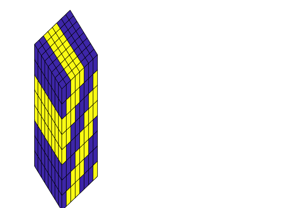
--------------------------------------------------------------------
Tarbert
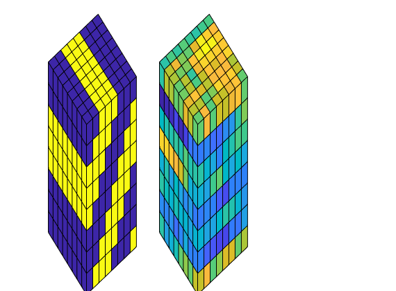
--------------------------------------------------------------------
Upper Ness
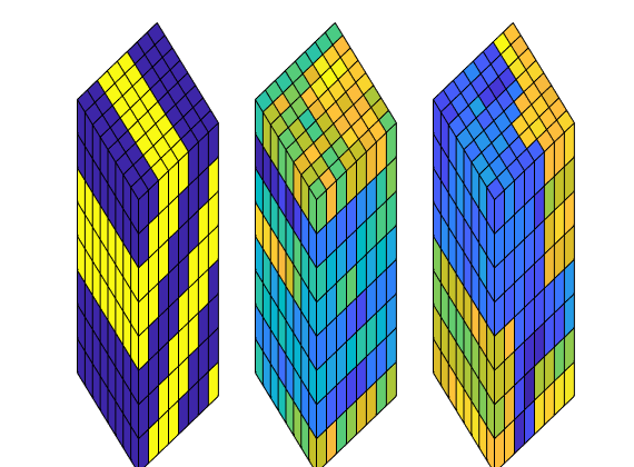
Upscale values
crock = cell(3,1);
% Harmonic-arithmetic
q = ones(G.cells.num,1);
vol = G.cells.volumes;
for i=1:size(rock.perm,2)
dims = G.cartDims; dims(i)=coarse(i);
qq = partitionUI(G, dims);
K = accumarray(qq,vol)./accumarray(qq,vol./rock.perm(:,i));
crock{1}.perm(:,i) = accumarray(q,K(qq).*vol)./accumarray(q,vol);
end
% Pressure drop
[v,dp] = deal(zeros(d, 1));
for i=1:d
bc = addBC([], bcl{i}.face, 'pressure', Dp{1});
bc = addBC(bc, bcr{i}.face, 'pressure', Dp{2});
xr = initResSol(G, 100*barsa, 1);
xr = incompTPFA(xr, G, hT, fluid, 'bc', bc);
v(i) = sum(xr.flux(bcr{i}.face)) / ...
sum(G.faces.areas(bcr{i}.face));
dp(i) = Dp{1}/L(i);
end
crock{2}.perm = fluid.properties()*(v./dp)';
% Periodic
v = nan(d);
dp = Dp{1}*eye(d);
nbcp = bcp;
for i=1:d
for j=1:d, nbcp.value(bcp.tags==j) = dp(j,i); end
xr = initResSol(Gp, 100*barsa, 1);
xr = incompTPFA(xr, Gp, hT, fluid, 'bcp', nbcp);
for j=1:d
v(j,i) = sum(xr.flux(ofaces{j})) / ...
sum(Gp.faces.areas(ofaces{j}));
end
end
dp = bsxfun(@rdivide, dp, L);
K = fluid.properties()*v/dp;
crock{3}.perm = abs(K([1 2 3 5 6 9]));
Compare upscaling
for j=1:numel(fl)
% Fine-scale problem
bc = pside([], G, fl{j}, barsa);
faces = bc.face;
if j<3
bc = pside(bc, G, fr{j}, 0);
else
cf = gridCellFaces(G,1);
cf = cf(any(G.faces.neighbors(cf,:)==0,2));
bc = addBC([], cf, 'pressure', barsa);
cf = gridCellFaces(G,G.cells.num);
cf = cf(any(G.faces.neighbors(cf,:)==0,2));
bc = addBC(bc, cf, 'pressure', 0);
end
x0 = initResSol(G,0);
xr = incompTPFA(x0, G, hT, fluid, 'bc', bc);
flux = sum(xr.flux(faces));
fprintf(' %5s -> %6s: ', fl{j}, fr{j});
for i=1:3
nrock.perm = crock{i}.perm(ones(G.cells.num,1),:);
chT = computeTrans(G, nrock);
x = incompTPFA(x0, G, chT, fluid, 'bc', bc);
fprintf('\t%f', sum(x.flux(faces)) / flux);
end
fprintf('\n');
end
East -> West: 0.784068 1.000000 1.025937
North -> South: 0.499741 1.000000 1.000000
Top -> Bottom: 1.042730 1.305649 1.342283
East -> West: 0.867555 1.000000 0.561113
North -> South: 0.892983 1.000000 0.538797
Top -> Bottom: 0.000034 0.000270 39.119231
East -> West: 0.830259 1.000000 0.401965
North -> South: 0.712832 1.000000 0.280813
Top -> Bottom: 0.095459 0.623773 2183.266271
end
disp('--------------------------------------------------------------------');
cax = caxis;
for i=1:3, subplot(1,3,i), caxis(cax); end
h = colorbar;
set(h,'Position',[0.94 0.1100 0.02 0.8150], ...
'XTick', .5, 'XTickLabel','[mD]', ...
'YTickLabel',num2str(10.^(-2:3)'));
Harm/arith Axial drop Periodic
--------------------------------------------------------------------
Upscale a problem with a diagonal trend
Generated from transmissibilityExample1.m
In this example we will upscale a problem with diagonal trend and compute the transmissibility associated with the coarse interface between two blocks in the x-direction
mrstModule add coarsegrid incomp;
Set up model
[Lx,Ly] = deal(200,100);
[nx,ny] = deal(30,15);
Dp = [1 0]*barsa;
G = computeGeometry(cartGrid([nx ny], [Lx Ly]));
rock = makeRock(G, 30*milli*darcy, 0.3);
rock.perm( sin(4*sum(G.cells.centroids(:,:),2)*pi/Lx)>0 ) = 10*milli*darcy;
rock.perm = rock.perm .* (1+.2*rand(size(rock.perm)));
hT = computeTrans(G, rock);
fluid = initSingleFluid('mu' ,1, 'rho', 1);
clf, plotCellData(G,rock.perm/(milli*darcy),'EdgeColor','none'); colorbar
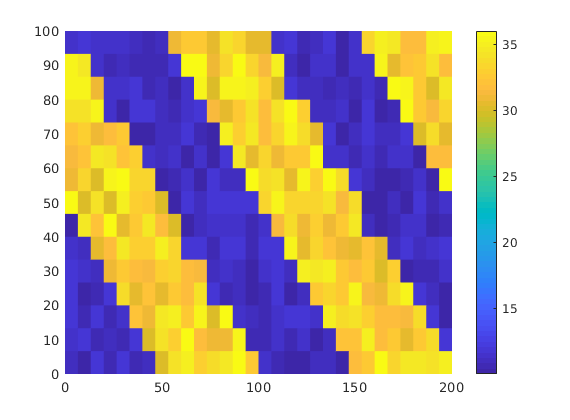
Solve fine-scale problem
bc = pside([], G, 'XMin', Dp(1));
bc = pside(bc, G, 'XMax', Dp(2));
xr = initResSol(G, 100*barsa, 1);
xr = incompTPFA(xr, G, hT, fluid, 'bc', bc);
Loop over various partititions
pow=4:-1:-2;
x = G.cells.centroids(:,1);
y = G.cells.centroids(:,2);
sp = [1 2 3 4 5 6 11];
clf, set(gcf,'Position',[360 500 930 300]);
for avg=[false, true]
T = zeros(size(pow));
for n=1:numel(pow);
% Find faces on coarse interface
q = (y> 50 + 2^pow(n)*(100-x))+1; q = q(:);
CG = generateCoarseGrid(G, q);
CG = coarsenGeometry(CG);
i = find(~any(CG.faces.neighbors==0,2));
faces = CG.faces.fconn(CG.faces.connPos(i):CG.faces.connPos(i+1)-1);
sgn = 2*(CG.faces.neighbors(i, 1) == 1) - 1;
% Upscale transmissibility
flux = sgn*sum(xr.flux(faces));
mu = fluid.properties();
if avg
P = accumarray(q,xr.pressure)./accumarray(q,1);
else
cells = findEnclosingCell(G,CG.cells.centroids);
P = xr.pressure(cells);
end
T(n) = mu*flux/(P(1) - P(2));
if avg, continue; end
% Plot grid
subplot(3,5,sp(n));
plotCellData(G,rock.perm(:,1),'EdgeColor','none');
plotGrid(CG,'FaceColor','none','LineWidth',1);
plotGrid(G, cells, 'FaceColor','k', 'EdgeColor','none');
axis equal off; axis([-1 201 -1 101]); title(num2str(n));
end
flag = true(15,1); flag(sp) = false;
subplot(3,5,find(flag)); hold on
if avg
plot(1:numel(pow),T,'--sb','LineWidth',1.5, 'MarkerSize',8, ...
'MarkerEdgeColor','k','MarkerFaceColor','r');
else
plot(1:numel(pow),T,'--or','LineWidth',1.5, 'MarkerSize',8, ...
'MarkerEdgeColor','k','MarkerFaceColor','b');
end
hold off
end
%axis([.5 7.5 [1.6 2.8]*1e-14]); legend('Centroid','Average',2);
colormap(.5*parula+.5*ones(size(parula)));
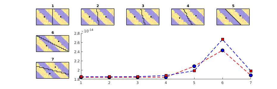
Illustrate use of flow diagnostics to verify upscaling
Generated from upscalingExample1.m
In this example we explain how to use match in cumulative well-allocation factors to verify the quality of an upscaling. In each well completion, the well-allocation factor is the percentage of the flux in/out of the completion that can be attributed to a pair of injection and production wells. The script can run two types of upscaling, if use_trans=false, we use a simple flow-based method to upscale permeability, while if use_trans=true, we use a more comprehensive method to upscale the transmissibilities and the well indices.
mrstModule add agglom upscaling coarsegrid diagnostics incomp;
use_trans = false;
Make model
We make a small model that consists of two different facies with contrasting petrophysical properties. An injector and a producer are placed diagonally opposite of each other and completed mainly in the high-permeable part of the model.
G = computeGeometry(cartGrid([40 20 15]));
K1 = gaussianField(G.cartDims, [200 2000]);
p1 = K1(:)*1e-4 + .2;
K1 = K1(:)*milli*darcy;
K2 = gaussianField(G.cartDims, [10 500]);
p2 = K2(:)*1e-4 + .2;
K2 = K2(:)*milli*darcy;
rad1 = G.cells.centroids(:,1).^2 + .5*G.cells.centroids(:,2).^2 ...
+ (G.cells.centroids(:,3)-2).^2;
rad2 = .5*(G.cells.centroids(:,1)-40).^2 + 2*G.cells.centroids(:,2).^2 ...
+ 2*(G.cells.centroids(:,3)-2).^2;
ind = ((rad1>600) & (rad1<1500)) | ((rad2>700) & (rad2<1400));
rock.perm = K2(:);
rock.perm(ind) = K1(ind);
rock.perm = bsxfun(@times, rock.perm, [1 1 1]);
rock.poro = p2(:);
rock.poro(ind) = p1(ind);
pv = poreVolume(G, rock);
W = verticalWell([], G, rock, 4, 17, 4:15, 'Comp_i', [1 0], ...
'Type', 'rate', 'Val', 0.2*sum(pv)/year, 'Name', 'I');
W = verticalWell(W, G, rock, 35, 3, 1:10, 'Comp_i', [0 1], ...
'Type', 'rate', 'Val', -0.2*sum(pv)/year, 'Name', 'P');
figure(1); clf,
set(gcf,'Position', [860 450 840 400],'PaperPositionMode','auto');
subplot(1,2,1);
plotCellData(G,rock.poro,'EdgeAlpha',.5); view(3);
plotWell(G,W,'Color','k'); axis off tight
pax = [min(rock.poro) max(rock.poro)];
[hc,hh] = colorbarHist(rock.poro, pax,'West');
pos = get(hh,'Position'); set(hh,'Position', pos - [.01 0 0 0]);
pos = get(hc,'Position'); set(hc,'Position', pos - [.03 0 0 0]);
set(gca,'Position',[.12 .075 .315 .9])
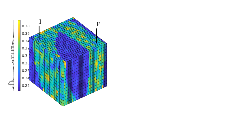
Compute flow on the fine-scale model
Transmissibility
hT = computeTrans(G, rock);
trans = 1 ./ accumarray(G.cells.faces(:,1), 1 ./ hT, [G.faces.num, 1]);
% Fluid model
dfluid = initSimpleFluid('mu' , [ 1, 10]*centi*poise , ...
'rho', [1014, 859]*kilogram/meter^3, ...
'n', [2 2]);
gravity reset off;
% Pressure solution
xd = initState(G, W, 100*barsa);
nw = numel(W);
xd = incompTPFA(xd, G, trans, dfluid, 'wells', W, 'use_trans', true);
Flow diagnostics on fine-scale model
To better reveal the communication in the reservoir, we subdivide each well into two segments, an upper and a lower segments, so that we altogether will have four well-pairs whose well-allocation factors can be used to verify the quality of the upscaling
nsegment=2;
[xd,Wdf] = expandWellCompletions(xd, W,[(1:nw)' repmat(nsegment,nw,1)]);
Df = computeTOFandTracer(xd, G, rock, 'wells', Wdf);
WPf = computeWellPairs(xd, G, rock, Wdf, Df);
Coarse-scale solution
We make a 5x5x15 coarse grid, in which we have chosen to keep the layering of the fine-scale model to simplify the comparison of well-allocation factors. Transmissibilities and well indices are upscaled using two slightly different methods: for the transmissibilities we use global generic boundary conditions and on each coarse face use the solution that has the largest flux orthogonal to the face to compute the upscaled transmissibility. For the wells, we use specific well conditions and use least squares for the flux.
p = partitionCartGrid(G.cartDims, [5 5 15]);
CG = coarsenGeometry(generateCoarseGrid(G, p));
crock = convertRock2Coarse(G, CG, rock);
if use_trans %#ok<*UNRCH>
[~,CTrans] = upscaleTrans(CG, hT, 'match_method', 'max_flux', ...
'bc_method', 'bc_simple');
[~,~,WC] = upscaleTrans(CG, hT, 'match_method', 'lsq_flux', ...
'bc_method', 'wells_simple', 'wells', W);
else
crock.perm = upscalePerm(G, CG, rock);
end
figure(1); subplot(1,2,2); cla
plotCellData(CG,crock.poro,'EdgeColor','none');
plotFaces(CG, boundaryFaces(CG),...
'EdgeColor', [0.4 0.4 0.4],'EdgeAlpha',.5, 'FaceColor', 'none'); view(3);
plotWell(G,W,'Color','k'); axis off tight
[hc,hh]=colorbarHist(crock.poro, pax,'East');
pos = get(hh,'Position'); set(hh,'Position', pos + [.01 0 0 0]);
pos = get(hc,'Position'); set(hc,'Position', pos + [.02 0 0 0]);
set(gca,'Position',[.56 .075 .315 .9])
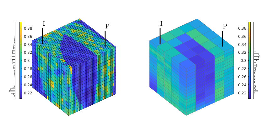
If permeability upscaling: to assess the effect of permeability upscaling only, we project the upscaled permeability back to the fine grid
if ~use_trans
crock.poro = crock.poro(p);
crock.perm = crock.perm(p,:);
CG = G;
WC = W;
CTrans = computeTrans(CG, crock);
CTrans = 1 ./ accumarray(CG.cells.faces(:,1), 1 ./ CTrans, [CG.faces.num, 1]);
p = (1:G.cells.num)';
end
xd = initState(CG, WC, accumarray(p,100*barsa)./accumarray(p,1));
xd = incompTPFA(xd, CG, CTrans, dfluid, 'wells', WC, 'use_trans', true);
Flow diagnostics on the upscaled model
Having obtained fluxes on the coarse model, we can expand the wells into two segments that exactly match the subdivision of in the fine-scale model and compute flow diagnostics.
nw = numel(WC);
[xdc,Wdc] = expandCoarseWellCompletions(xd, WC, Wdf, p);
Dc = computeTOFandTracer(xdc, CG, crock, 'wells', Wdc);
WPc = computeWellPairs(xdc, CG, crock, Wdc, Dc);
nit = numel(Df.inj);
npt = numel(Df.prod);
nseg = nit + npt;
Display bar charts of flow-allocation factors
For each well segment, we plot bar chart of the cumulative flux in/out of the completions that make up the segment, from bottom to top. In the plots, each well segment is assigned a unique color and each bar is subdivided into the fraction of the total in/outflux that blongs to the different well-pairs the segment is part of. The plots show the allocation factors for the upper half of the injector (I:1, upper-left plot), the lower part of the injector (I:2, upper-right plot), the upper part of the producer (P:1, lower-left plot), and the lower part of the producer (P:2, lower-right plot). Looking at the bar chart for I:1, we see that the majority of the flux from this injector is colored yellow and hence goes to P:1, which corresponds to the upper part of the producer.
figure(2); set(gcf,'Position', [860 450 840 400]); clf
plotWellAllocationComparison(Dc, WPc, Df, WPf);
dy = [-.05 -.05 -.025 -.025];
dx = [-.5 0 -.5 0 0];
for i=1:4
subplot(2,2,i);
pos = get(gca,'Position');
pos = pos + [-.05 dy(i) .075 .075];
set(gca,'Position',pos,'XTick',[],'YTick',[]);
end
cmap = jet(nseg); cmap = 0.6*cmap + .4*ones(size(cmap)); colormap(cmap);
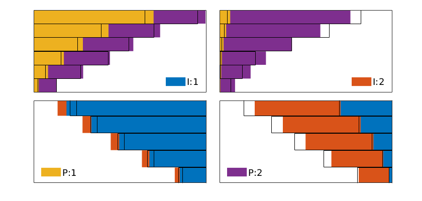
Display the partition
Last we show the cells that belong to the four different well segments and show the corresponding injector/producer partitions. We can now compare the partitions with the well-allocation factors in Figure 2. Let us take the allocation for I:2 as an example. In the upper-right plot of Figure 2 we see that almost all the flux from this injector goes to P:2. Looking at the cyan region in the left plot of Figure 1 confirms this: this region is hardly in contact with the yellow segment of the producer. The blue region, on the other hand, contains both the upper segment of the producer (P:1, yellow color) and parts of the lower segment (P:2, red color). Likewise, the red volume in the right-hand plot of Figure 3 covers both the lower segment of the injector (I:2, cyan) and parts of the upper segment (I:1, blue). In the bars of P:2 to the lower-right in Figure 2, we therefore see that relatively large portion of the bars are in blue color.
oG = computeGeometry(cartGrid([1 1 1],[40 20 15]));
figure(3); clf
set(gcf,'Position', [860 450 840 310],'PaperPositionMode','auto');
subplot(1,2,1);
for i=1:nit
plotCellData(G,Df.ipart,Df.ipart==i,'FaceAlpha',.3,'EdgeAlpha',.2);
end
plotGrid(oG,'FaceColor','none');
for i=1:nseg,
plotGrid(G,Wdf(i).cells,'FaceColor',cmap(i,:));
end
plotWell(G,W,'Color','k');
view(-40,10); axis tight off; caxis([1 nit+npt]);
subplot(1,2,2);
for i=1:npt
plotCellData(G,Df.ppart+nit,Df.ppart==i,'FaceAlpha',.4,'EdgeAlpha',.2);
end
plotGrid(oG,'FaceColor','none');
for i=1:nseg,
plotGrid(G,Wdf(i).cells,'FaceColor',cmap(i,:));
end
plotWell(G,W,'Color','k');
view(-40,10); axis tight off; caxis([1 nit+npt]);
colormap(cmap);
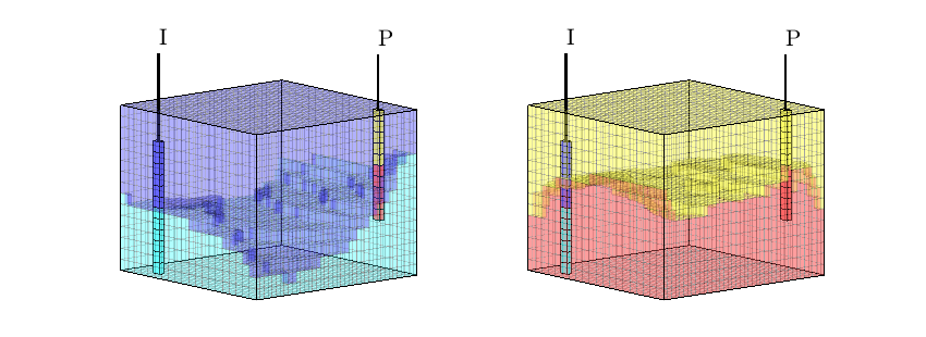
Upscaling workflow
Generated from upscalingExample3.m
This example aims to show the complete workflow for creating, running and analyzing a simulation model. Unlike the other examples, we will create all features of the model manually to get a self-contained script without any input files required. The model we setup is a slightly compressible two-phase oil/water model with multiple wells. The reservoir has a layered strategraphy consisting of three layered sections, four layers with different permeability, and three major faults. Note that this example features a simple conceptual model designed to show the workflow rather than a problem representing a realistic scenario in terms of well locations and fluid physics.
mrstModule add ad-core ad-blackoil ad-props diagnostics mrst-gui
close all;
Horizons for internal and external geology
We begin by building the horizons that define the top and bottom structure of the sector, as well as two internal erosions.
% Define areal mesh
[xmax,ymax, n] = deal(1000*meter, 1000*meter, 30);
[x, y] = meshgrid(linspace(0,xmax,n+1), linspace(0,ymax,n+1));
[x, y] = deal(x',y');
% Basic dome structure
dome = 1-exp(sqrt((x - xmax/2).^2 + (y - ymax/2).^2)*1e-3);
% Periodic perturbation
[xn,yn] = deal(pi*x/xmax,pi*y/ymax);
perturb = sin(5*xn) + .5*sin(4*xn+6*yn) + cos(.25*xn*yn./pi^2) + cos(3*yn);
perturb = perturb/3.5;
% Random small-scale perturbation
rng(0);
[h, hr] = deal(8,1);
zt = 50 + h*perturb + rand(size(x))*hr - 20*dome;
zb = zt + 30;
zmb = min(zb + 4 + 0.01*x - 0.020*y + hr*rand(size(x)), zb);
zmt = max(zb -15 + 0.01*x - 0.025*y + hr*rand(size(x)), zt);
horizons = {struct('x', x, 'y', y, 'z', zt), ...
struct('x', x, 'y', y, 'z', zmt), ...
struct('x', x, 'y', y, 'z', zmb), ...
struct('x', x, 'y', y, 'z', zb)};
surf(x,y,zt-.2, 'EdgeC','r','FaceC',[.8 .8 .8]), hold on
mesh(x,y,zmt-.2,'EdgeC','g','FaceC',[.7 .7 .7]),
mesh(x,y,zmb-.2,'EdgeC','g','FaceC',[.6 .6 .6]),
mesh(x,y,zb-.2, 'EdgeC','b','FaceC',[.5 .5 .5]); hold off
set(gca,'ZDir','reverse')
view(-50,10); axis off
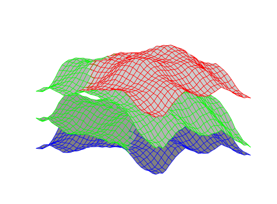
Interpolate to build unfaulted corner-point grid
dims = [40, 40]; layers = [3 6 3];
grdecl = convertHorizonsToGrid(horizons, 'dims', dims, 'layers', layers);
G = processGRDECL(grdecl);
[~,~,k] = gridLogicalIndices(G);
figure, plotCellData(G,k,'EdgeAlpha',.2); view(3);
colormap(.5*jet + .5*ones(size(jet)));
view(-50,30); axis off
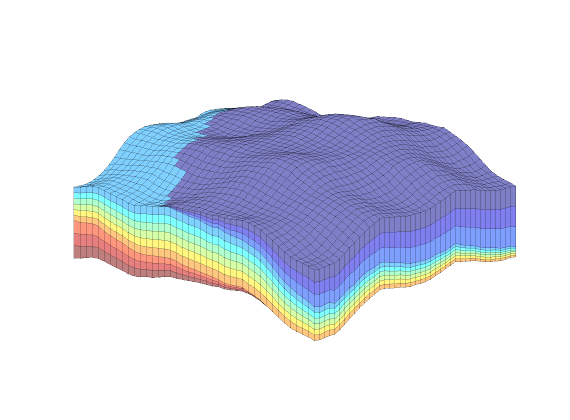
Insert faults
[X,Y,Z] = buildCornerPtNodes(grdecl);
i=47:80; Z(i,:,:) = Z(i,:,:) + .022*min(0,Y(i,:,:)-550);
j= 1:30; Z(:,j,:) = Z(:,j,:) + .021*min(0,X(:,j,:)-400);
j=57:80; Z(:,j,:) = Z(:,j,:) + .023*min(0,X(:,j,:)-750);
grdecl.ZCORN = Z(:);
G = processGRDECL(grdecl);
G = computeGeometry(G);
[~,~,k] = gridLogicalIndices(G);
figure, plotCellData(G,k,'EdgeAlpha',.2); view(3);
plotFaces(G,find(G.faces.tag>0),'EdgeColor','r','FaceColor',[.8 .8 .8]);
colormap(.5*jet + .5*ones(size(jet)));
view(-50,30); axis tight off
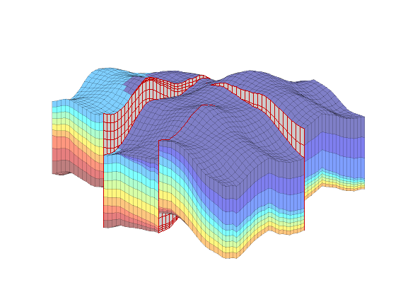
Petrophysics
Set up permeability based on K-indices and introduce anisotropy by setting K_z = .1*K_x
rng(357371);
[K,L] = logNormLayers(G.cartDims, [100 400 10 50]*milli*darcy);
K = K(G.cells.indexMap);
perm = [K, K, 0.1*K];
rock = makeRock(G, perm, 0.3);
% Plot horizontal permeability
figure
K = convertTo(K,milli*darcy);
plotCellData(G, log10(K),'EdgeAlpha',.1)
colorbarHist(K,[1 1500],'South',100,true);
view(-50, 50), axis tight off
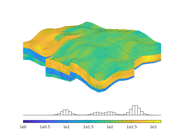
Define wells
Hydrocarbon is recovered from producers, operating at fixed bottom-hole pressure and perforated throughout all layers of the model. The producers are supported by a single water injector set to inject one pore volume over 10 years (the total simulation length).
% Producers
simTime = 10*year;
pv = poreVolume(G, rock);
injRate = 1*sum(pv)/simTime;
offset = 10;
W = verticalWell([], G, rock, offset, offset, [],...
'Name', 'P1', 'comp_i', [1 0], ...
'Val', 250*barsa, 'Type', 'bhp', 'refDepth', 50);
W = verticalWell(W, G, rock, offset, floor(G.cartDims(1)/2)+3, [],...
'Name', 'P2', 'comp_i', [1 0], ...
'Val', 250*barsa, 'Type', 'bhp', 'refDepth', 50);
W = verticalWell(W, G, rock, offset, G.cartDims(2) - offset/2, [], ...
'Name', 'P3', 'comp_i', [1 0], ...
'Val', 250*barsa, 'Type', 'bhp', 'refDepth', 50);
% Injectors
W = verticalWell(W, G, rock, G.cartDims(1)-5, offset, [],...
'Name', 'I1', 'comp_i', [1 0], ...
'Val', injRate, 'Type', 'rate', 'refDepth', 50);
% Plot the wells
plotWell(G, W,'color','k')
axis tight
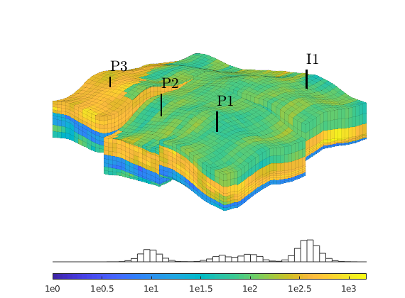
Define fluid behavior and instantiate model
We set up a two-phase oil-water simulation model based on automatic differentiation. The resulting object is a special case of a general three-phase model and to instantiate it, we start by constructing a three-phase fluid structure with properties given for oil, water, and gas. (The gas properties will be neglected once we construct the two-phase object). Water is assumed to be incompressible, whereas oil has constant compressibility, giving an expansion factor of the form,
. To define this relation, we set the ‘bo’ field of the fluid structure to be an anonymous function that calls the builtin ‘exp’ function with appropriate arguments. Since the fluid model is a struct containing function handles, it is simple to modify the fluid to use alternate functions. We then pass the fundamental structures (grid, rock and fluid) onto the two-phase oil/water model constructor.
% Three-phase template model
fluid = initSimpleADIFluid('mu', [1, 5, 0]*centi*poise, ...
'rho', [1000, 700, 0]*kilogram/meter^3, ...
'n', [2, 2, 0]);
% Constant oil compressibility
c = 0.001/barsa;
p_ref = 300*barsa;
fluid.bO = @(p, varargin) exp((p - p_ref)*c);
% Construct reservoir model
gravity reset on
model = TwoPhaseOilWaterModel(G, rock, fluid);
Define initial state
Once we have a model, we need to set up an initial state. We set up a very simple initial state; we let the bottom part of the reservoir be completely water filled, and the top completely oil filled. MRST uses water, oil, gas ordering internally, so in this case we have water in the first column and oil in the second for the saturations.
depthOW = 85*meter;
depthD = 10*meter;
region = getInitializationRegionsBlackOil(model, depthOW, ...
'datum_depth', depthD, 'datum_pressure', p_ref);
state0 = initStateBlackOilAD(model, region);
figure
plotCellData(G, state0.s(:,1),'EdgeAlpha',.1), colormap(flipud(winter));
plotWell(G,W,'color','k')
patch([-50 1050 1050 -50],[-50 -50 1050 1050],depthOW*ones(1,4), ...
ones(1,4), 'FaceColor',[.6 .6 1],'EdgeColor','r','LineWidth',1);
view(-50, 50), axis tight off
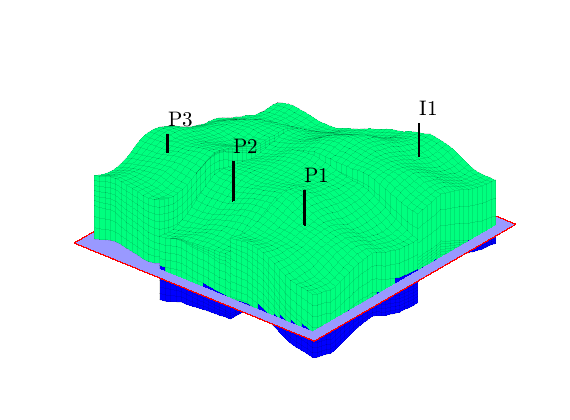
Define simulation schedule and set solver parameters
We define a relatively simple schedule consisting of five small control steps initially, followed by 25 larger steps. We keep the well controls fixed throughout the simulation. To accelerate the simulation, we set somewhat stricter tolerances and use a CPR preconditioner with an algebraic multigrid solver (agmg) for the elliptic pressure system
% Compute the timestep
nstep = 25;
refine = 5;
startSteps = repmat((simTime/(nstep + 1))/refine, refine, 1);
restSteps= repmat(simTime/(nstep + 1), nstep, 1);
timesteps = [startSteps; restSteps];
% Set up the schedule containing both the wells and the timestep
schedule = simpleSchedule(timesteps, 'W', W);
% Tighten tolerences
model.drsMaxRel = inf;
model.dpMaxRel = .1;
model.dsMaxAbs = .1;
% Set up CPR preconditioner
try
mrstModule add agmg
pressureSolver = AGMGSolverAD('tolerance', 1e-4);
catch
pressureSolver = BackslashSolverAD();
end
linsolve = CPRSolverAD('ellipticSolver', pressureSolver, 'relativeTolerance', 1e-3);
No module mapping found for
* agmg
Simulate base case
We now have an intial state, the schedule defines dynamic controls and time steps, and the model gives the mathematical description of how to advance the solution one time step. We then have all we need to simulate the problem. Because the simulation will consume some time, we launch a progress report and a plotting tool for the well solutions (well rates and bottom-hole pressures)
fn = getPlotAfterStep(state0, model, schedule,'view',[50 50], ...
'field','s:1','wells',W);
[wellSols, states, report] = ...
simulateScheduleAD(state0, model, schedule, ...
'LinearSolver', linsolve, 'afterStepFn',fn);
Solving timestep 01/30: -> 28 Days, 1 Hour, 3046.15 Seconds
Warning: Matrix is close to singular or badly scaled. Results may be inaccurate.
RCOND = 1.216893e-16.
Warning: Matrix is close to singular or badly scaled. Results may be inaccurate.
RCOND = 1.216893e-16.
Warning: Matrix is close to singular or badly scaled. Results may be inaccurate.
RCOND = 1.216893e-16.
Warning: Matrix is close to singular or badly scaled. Results may be inaccurate.
...
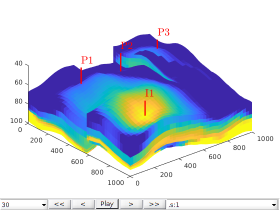
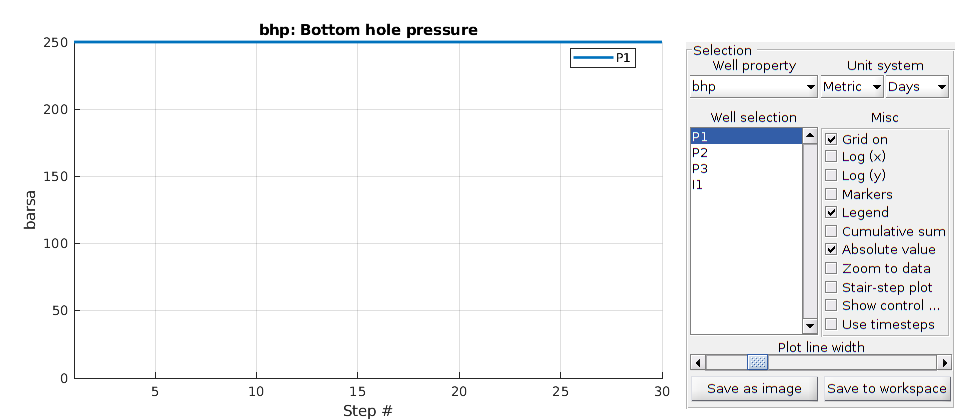
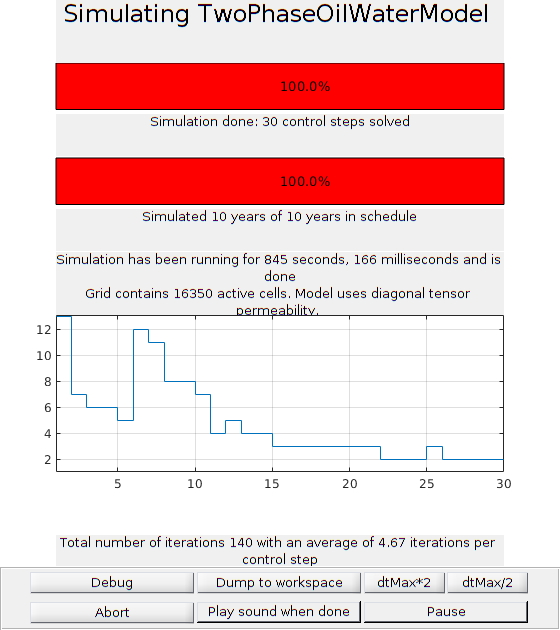
Plot reservoir states
We launch a plotting tool for the reservoir quantities (pressures and saturations, located in states).
figure, plotToolbar(G, states)
view(50, 50);
plotWell(G,W);
figure
mrstModule add coarsegrid
CG = generateCoarseGrid(G,ones(G.cells.num,1));
plotWell(G, W,'color','k')
plotFaces(CG,1:CG.faces.num,'EdgeColor','k','FaceColor','none','LineWidth',2);
s=states{6}.s(:,1); plotCellData(G,s,s>1e-2); caxis([0 1]);
colormap(flipud(winter)), view(-53,46); axis tight off
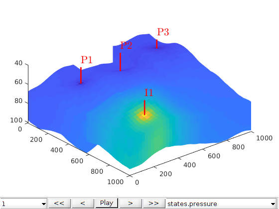
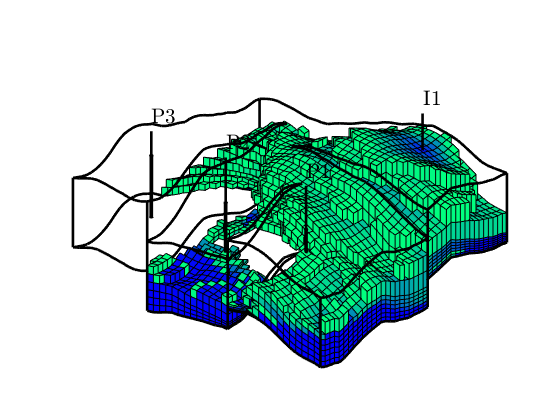
Launch flow diagnostics
interactiveDiagnostics(G, rock, W, 'state', states{end}, 'computeFlux', false);
set(gcf,'position',[440 317 866 480]); axis normal
view(-85,73)
New state encountered, computing diagnostics...

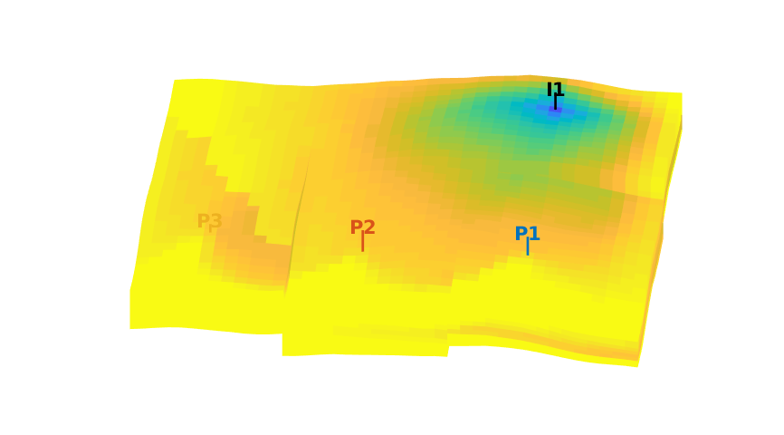
Create an upscaled, coarser model
The fine scale model has 16 350 cells. If we want a smaller model we can easily define an upscaled model. We start by setting up a straightforward uniform partition of the IJK-indices. This gives 1388 coarse blocks (after a postprocessing to split disconnected blocks), which corresponds to more than 20 times reduction in the number of unknowns.
mrstModule add coarsegrid
cdims = [10, 10, 12];
p0 = partitionUI(G, cdims);
% p0 = partitionLayers(G, cdims(1:2), L);
figure;
CG = generateCoarseGrid(G,p0);
plotGrid(G,'FaceColor',[1 .8 .9],'EdgeAlpha',.1);
plotFaces(CG,1:CG.faces.num,'EdgeColor','k','FaceColor','none','LineWidth',1.5);
axis tight off, view(125, 55)
title('Straightforward index partition');
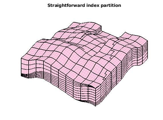
Split blocks over the fault lines
The partition above may give blocks that have cells on opposite sides of a fault. To ensure that as many as possible of the coarse blocks are hexahedral (except for those that are partially eroded), we split blocks that have cells on both sides of a fault. To do this, we introduce a temporary grid in which the faults act as barriers, and then perform a simple postprocessing to split any coarse blocks intersected by one of the faults. Afterwards, we show the new partition and highlight blocks created due to the modification of the fault.
Gf = makeInternalBoundary(G, find(G.faces.tag > 0));
p = processPartition(Gf, p0);
plotGrid(G,p>prod(max(p0)),'FaceColor','g','EdgeColor','none');
title('Splitting over fault lines');
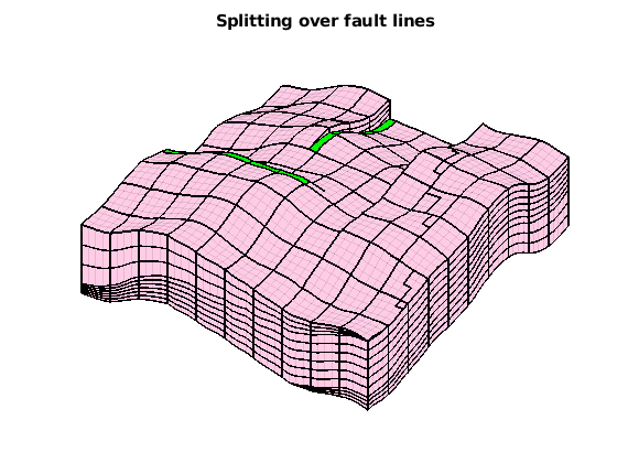
Upscale the model and simulate the coarser problem
We can now directly upscale the model, schedule, and initial state. By default, the upscaling routine uses the simplest possible options, i.e., harmonic averaging of permeabilities. It is possible to use more advanced options, but for the purpose of this example we will use the defaults.
modelC1 = upscaleModelTPFA(model, p);
scheduleC1 = upscaleSchedule(modelC1, schedule);
state0C1 = upscaleState(modelC1, model, state0);
% Plot the initial state
figure,
GC = modelC1.G;
rockC = modelC1.rock;
plotCellData(GC,state0C1.s(:,1),'EdgeColor','none'), colormap(flipud(winter));
plotWell(G,W,'color','k')
plotFaces(GC,1:GC.faces.num,'FaceColor','none');
patch([-50 1050 1050 -50],[-50 -50 1050 1050],85*ones(1,4), ...
ones(1,4), 'FaceColor',[.6 .6 1],'EdgeColor','r','LineWidth',1);
view(-50, 50), axis tight off
% Once we have an upscaled model, we can again simulate the new schedule
% and observe that the time taken is greatly reduced, even without the use
% of a CPR preconditioner.
[wellSolsC1, statesC1] = simulateScheduleAD(state0C1, modelC1, scheduleC1);
Solving timestep 01/30: -> 28 Days, 1 Hour, 3046.15 Seconds
Solving timestep 02/30: 28 Days, 1 Hour, 3046.15 Seconds -> 56 Days, 3 Hours, 2492.31 Seconds
Solving timestep 03/30: 56 Days, 3 Hours, 2492.31 Seconds -> 84 Days, 5 Hours, 1938.46 Seconds
Solving timestep 04/30: 84 Days, 5 Hours, 1938.46 Seconds -> 112 Days, 7 Hours, 1384.62 Seconds
Solving timestep 05/30: 112 Days, 7 Hours, 1384.62 Seconds -> 140 Days, 9 Hours, 830.77 Seconds
Solving timestep 06/30: 140 Days, 9 Hours, 830.77 Seconds -> 280 Days, 18 Hours, 1661.54 Seconds
Solving timestep 07/30: 280 Days, 18 Hours, 1661.54 Seconds -> 1 Year, 56 Days, 3.69 Hours
Solving timestep 08/30: 1 Year, 56 Days, 3.69 Hours -> 1 Year, 196 Days, 12.92 Hours
...
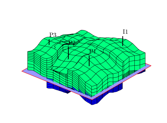
Create a second upscaled model with flow-based upscaling
We use the upscaling module to create a tailored upscaled model. This upscaling routine uses an incompressible flow field with the wells of the problem to perform a global upscaling.
mrstModule add incomp agglom upscaling
[~, TC, WC] = upscaleTrans(GC, model.operators.T_all, ...
'Wells', W, 'bc_method', 'wells', 'fix_trans', true);
modelC2 = upscaleModelTPFA(model, p, 'transCoarse', TC);
scheduleC2 = schedule;
for i = 1:numel(scheduleC2.control)
scheduleC2.control(i).W = WC;
end
[wellSolsC2, statesC2] = simulateScheduleAD(state0C1, modelC2, scheduleC2);
Upscaled transmissibility does not reproduce upscaling scenario. Results may be inaccurate.
Pressure solve 1/1 with upscaled transmissibility does not give comparable results
Warning: Set boundary face trans to zero
Solving timestep 01/30: -> 28 Days, 1 Hour, 3046.15 Seconds
Solving timestep 02/30: 28 Days, 1 Hour, 3046.15 Seconds -> 56 Days, 3 Hours, 2492.31 Seconds
Solving timestep 03/30: 56 Days, 3 Hours, 2492.31 Seconds -> 84 Days, 5 Hours, 1938.46 Seconds
Solving timestep 04/30: 84 Days, 5 Hours, 1938.46 Seconds -> 112 Days, 7 Hours, 1384.62 Seconds
Solving timestep 05/30: 112 Days, 7 Hours, 1384.62 Seconds -> 140 Days, 9 Hours, 830.77 Seconds
...
Compare the well solutions
plotWellSols({wellSols, wellSolsC1, wellSolsC2}, cumsum(schedule.step.val), ...
'DatasetNames', {'Fine scale', 'Harmonic', 'Flow-based'}, 'Field', 'qOs');
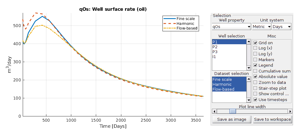
Compute flow diagnostics
As an alternative to looking at well curves, we can also look at the flow diagnostics of the models. Flow diagnostics are simple routines based on time-of-flight and tracer equations, which aim to give a qualitative understanding of reservoir dynamics. Here, we take the state after a single time step as a snapshot for both the fine and coarse model and compute time-of-flight and well tracers.
mrstModule add diagnostics
D = computeTOFandTracer(states{2}, G, rock, 'Wells', schedule.control.W);
DC1 = computeTOFandTracer(statesC1{2}, GC, rockC, 'Wells', scheduleC1.control.W);
DC2 = computeTOFandTracer(statesC2{2}, GC, rockC, 'Wells', scheduleC1.control.W);
WP = computeWellPairs(states{1}, G, rock, schedule.control.W, D);
WPC1 = computeWellPairs(statesC1{1}, GC, rockC, scheduleC1.control.W, DC1);
WPC2 = computeWellPairs(statesC2{1}, GC, rockC, scheduleC1.control.W, DC2);
figure, plotWellAllocationComparison(DC1, WPC1, D, WP);%, 'plotrow', true);
figure, plotWellAllocationComparison(DC2, WPC2, D, WP);%, 'plotrow', true);
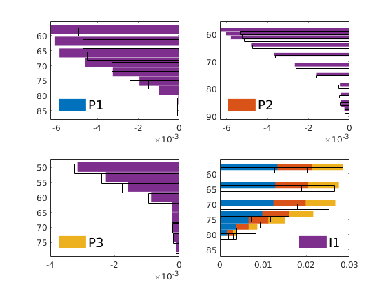
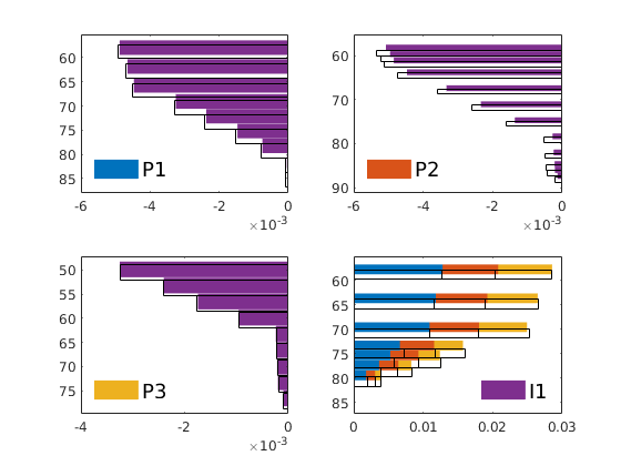
Copyright notice
<html>
% <p><font size="-1