`co2lab`: Numerical CO₂ laboratory¶

The MRST Numerical CO2 Laboratory combines results of more than one decade of academic research and development of mathematical models and numerical methods for CO2 storage modeling combined into a unified toolchain that is easy and intuitive to use. The software is flexible and efficient and can be used to study realistic injection scenarios, or function as a platform for rapid prototyping of new models and computational methods.

Different vertical equilibrium models are included, ranging from simple incompressible immiscibile two-phase models to compressible models with CO2 dissolution. A range of interactive tools makes it easy to visualize how CO2 will migrate and behave under different conditions and for different saline aquifers.

The module offers:

simplified access to public data sets from the CO2 Storage Atlas of the Norwegian Continental Shelf
identification of structural traps and computation of storage capacity estimates
vertical-equilibrium methods specifically to study long-term, large-scale migration
detailed carbon trapping inventories
a large number of tutorials and examples
optimization methods
complete simulation setups from published papers, to support reproducible research

Contents¶

INTERACTIVE_TOOLS

Files: exploreCapacity - opt - structure containing variables that can be overridden by user at exploreSimulation - Undocumented Utility Function interactiveTrapping - Create an interactive figure showing trapping structure for a top surface grid

exploreCapacity(varargin)¶

opt - structure containing variables that can be overridden by user at: command line
var - structure containing variables that user cannot override at command: line

exploreSimulation(varargin)¶: Undocumented Utility Function

interactiveTrapping(inp, varargin)¶

Create an interactive figure showing trapping structure for a top surface grid

For a detailed list of functionality and controls, please see the showTrapsInteractively example.

Synopsis:

interactiveTrapping('Johansenfm')
interactiveTrapping(G_top)

Parameters:

inp – Either a valid top surface grid as defined by topSurfaceGrid(G) or a string which is valid input for getAtlasGrid.
'pn'/pv –
List of optional property names/property values:
- coarsening: If inp is the name of a Atlas grid, this argument will be passed onto getAtlasGrid to coarsen the surface. Default: 1 for the full grid.
- light: toggle the lighting of the surface grid. Default: false
- spillregions: toggle the display of spill regions on the surface grid Default: false
- traps: toggle the display of traps on the surface grid Default: true
- colorpath: toggle red/gray color scheme to mark the traps encountered along a spill path; same color is applied on the histogram of trapping volumes. Default: true
- method: Choose cell or node based algorithm. Valid inputs: ‘node’, ‘cell’. Default: ‘cell’.
- injpt: Choose this cell number as injection point at startup. If zero, no injection point is selected. Default: zero
- contour: toggle drawing of contour lines of height data if these are available as part of the data set

Returns:

h – Handle to resulting figure object.

See also

trapAnalysis, showTrapsInteractively

Contents¶

HELPERS

Files: getMigrationTree - Recursively traverse and find the full migration tree

getMigrationTree(G, A, trap, depth)¶: Recursively traverse and find the full migration tree

Contents¶

UTILS

Files: visualSimulation - Undocumented Utility Function

visualSimulation(initState, model, schedule, varargin)¶: Undocumented Utility Function

Contents¶

EQUATIONS

Files: addFluxesFromSourcesAndBCSens - Add in fluxes imposed by sources and face boundary conditions equationsWaterGas - { equationsWGVEbasic - { equationsWGVEbasicSens - { equationsWGVEdisgas - { getBoundaryConditionFluxesADSens - Get boundary condition fluxes for a given set of values

addFluxesFromSourcesAndBCSens(model, eqs, pressure, rho, mob, b, s, forces, permfac, dz)¶

Add in fluxes imposed by sources and face boundary conditions

Description:

Utility function for updating residual conservation equations in the AD framework with additional fluxes due to boundary conditions and sources. Wells are handled separately in WellModel.

Parameters:

model – Simulation model (subclass of ReservoirModel).
eqs –

Residual conservation of mass-equations for each phase, in

the order WATER, OIL, GAS (with any inactive phases omitted) as a cell array.

(All the following arguments are cell arrays, with length equal to the number of the active phases, with the values for each cell in each entry unless otherwise noted)

pressure - Phase pressures rho - Surface densities (one value per phase) mob - Phase mobilities b - Phase b-factors (volume in reservoir to standard conditions) s - Phase saturations

forces - Struct containing .src and .bc fields for sources and

boundary conditions respectively.

Returns:

eqs – Phase conservation equations with added fluxes.
qBC – Phase fluxes due to BC at standard conditions.
BCTocellMap – Matrix mapping qBC to cells.
qSRC – Phase fluxes due to source terms.
srcCells – List of cells, mapping qSRC to cells.

getBoundaryConditionFluxesADSens(model, pressure, rho, mob, b, s, bc, permfac, dz)¶

Get boundary condition fluxes for a given set of values

Synopsis:

[qSurf, BCTocellMap, BCcells] = getBoundaryConditionFluxesAD(model, pressure, rho, mob, b, s, bc)

Description:

Given a set of boundary conditions, this function computes the fluxes induced for a given set of reservoir parameters (density, mobility, saturations etc).

Parameters:

model – Subclass of ReservoirModel implementing the current simulation model.
pressure – Cell values of pressure. Should be a nph long cell array, containing the phase pressures.
rho – Surface densities of each phase, as a nph long cell array.
b – Reservoir to standard condition factors per phase, as a nph long array.
s – Phase saturations per cell, as a nph long array.
bc – Boundary condition struct, with valid .sat field with length nph. Typically made using addBC, pside or fluxside.

Returns:

qSurf – Cell array of phase fluxes.
BCTocellMap – Matrix used to add in bc fluxes to cells. Implemented as a matrix to efficiently account for cells with multiple faces with boundary conditions.
cells – The cells affected by boundary conditions.

See also

addBC, pside, fluxside

Contents¶

UTILS

Files: getPhaseFluxAndProps_WGVE - Function to compute phase fluxes, volume factors, mobilities, getPhaseFluxAndProps_WGVEsens - Function to compute phase fluxes, volume factors, mobilities,

getPhaseFluxAndProps_WGVE(model, pW, pG, krX, T, gdz, phase, rs, temp)¶: Function to compute phase fluxes, volume factors, mobilities, densities, upstream indices and pressure gradients

getPhaseFluxAndProps_WGVEsens(model, pW, pG, krX, T, gdz, phase, rs, temp, rhofac)%, permfac, porofac)¶: Function to compute phase fluxes, volume factors, mobilities, densities, upstream indices and pressure gradients

Contents¶

FLUIDS

Files: addVE3DRelperm - addVEBlackOilRelperm - addVERelperm - Add VE-upscaled rel.perm. (and related functions) for a two-phase fluid addVERelperm1DTables - { addVERelperm1DTablesPressure - { addVERelpermCapLinear - VE relperm with linear capillary pressure addVERelpermIntegratedFluid - { addVERelpermSens - Add VE-upscaled rel.perm. (and related functions) for a two-phase fluid object free_sg - Determine the mobile part of present saturation. ifcond - this function should be expanded makeVEFluid - Construct a VE fluid with properties specific to a chosen model makeVEFluidSens - Construct a VE fluid with properties specific to a chosen model makeVEFluidsForTest - { makeVEtables - { minRs - Determine the minimal amount of dissolved CO2 in each cell, based on the veRelpermTester - { veRelpermTesterCell - {

addVERelperm(fluid, Gt, varargin)¶

Add VE-upscaled rel.perm. (and related functions) for a two-phase fluid object and the sharp-interface assumption.

Synopsis:

function fluid = addVERelperm(fluid, varargin)

DESCRIPTION: Add VE-upscaled relative permeability functions and capillary pressure function for a two-phase fluid object (water and CO2).

Parameters:

fluid – Fluid object to modify
Gt – Top surface grid
varargin –
Option/value pairs, where the following options are available: res_water - residual oil saturation (scalar) res_gas - residual gas saturation (scalar) krw - rel. perm of water at full flowing saturation krg - rel. perm of gas at full flowing saturation top_trap - Thickness of sub-resolution caprock rugosity surf_topo - Sub-resolution rugosity geometry type. Can be

’smooth’, ‘square’, ‘sinus’ or ‘inf_rough’.

Returns:

fluid – The modified fluid object, endowed with the additional
functions/fields
res_gas – residual gas saturation (scalar)
res_water – residual oil saturation (scalar)
krG – upscaled rel.perm. of gas as a function of (gas) saturation
krW – upscaled rel.perm. of water as a function of (water) saturation
pcWG – upscaled ‘capillary pressure’ as a function of gas saturation
invPc3D – Fine-scale water saturation as function of cap. pressure
kr3D – Dummy function, returning a rel.perm. value that is simply equal to the input saturation.

addVERelpermCapLinear(fluid, cap_scale, varargin)¶: VE relperm with linear capillary pressure

addVERelpermSens(fluid, Gt, varargin)¶

Add VE-upscaled rel.perm. (and related functions) for a two-phase fluid object

Synopsis:

function fluid = addVERelperm(fluid, varargin)

DESCRIPTION: Add VE-upscaled relative permeability functions and capillary pressure function for a two-phase fluid object (water and CO2).

Parameters:

fluid – Fluid object to modify
Gt – Top surface grid
varargin –
Option/value pairs, where the following options are available: res_water - residual oil saturation (scalar) res_gas - residual gas saturation (scalar) krw - rel. perm of water at full flowing saturation krg - rel. perm of gas at full flowing saturation top_trap - Thickness of sub-resolution caprock rugosity surf_topo - Sub-resolution rugosity geometry type. Can be

’smooth’, ‘square’, ‘sinus’ or ‘inf_rough’.

Returns:

fluid – The modified fluid object, endowed with the additional
functions/fields
res_gas – residual gas saturation (scalar)
res_water – residual oil saturation (scalar)
krG – upscaled rel.perm. of gas as a function of (gas) saturation
krW – upscaled rel.perm. of water as a function of (water) saturation
pcWG – upscaled ‘capillary pressure’ as a function of gas saturation
invPc3D – Fine-scale water saturation as function of cap. pressure
kr3D – Dummy function, returning a rel.perm. value that is simply equal to the input saturation.

free_sg(sg, sGmax, opt)¶

Determine the mobile part of present saturation.

Synopsis:

function fsg = free_sg(sg, sGmax, opt)

DESCRIPTION: Assuming a sharp interface, this function determine the amount of present saturation that is in the ‘mobile plume’ domain (as opposed to the region below the mobile plume where CO2 has been residually trapped after imbibition. As such, the “mobile part of present saturation” does include the CO2 in the mobile plume that is destined to be left behind as residual trapping, but not the CO2 that is already residually trapped.

The formula is based on the simple transformation:: s * H = h * (1 - sr(2)) + (h_max - h) * sr(1)

s_max * H = h_max * (1 - sr(2))

Parameters:	sg – present saturation sGmax – historically maximum saturation opt – structure expected to contain the following fields: * opt.res_gas : residual gas saturation * opt.res_water : residual oil saturation
Returns:	fsg – the free part of the present saturation (fsg <= sg)

ifcond(u, v, cond)¶: this function should be expanded

makeVEFluid(Gt, rock, relperm_model, varargin)¶

Construct a VE fluid with properties specific to a chosen model

Synopsis:

function fluid = makeVEFluid(Gt, rock, relperm_model, varargin)

DESCRIPTION:

Parameters:

Gt – Underlying top-surface grid with which the fluid object will be used.
rock – Object holding the vertically-averaged rock properties of Gt (can be obtained from a normal rock structure using the ‘averageRock’ function in CO2lab).
relperm_model –
Text string used to specify one of several possible models for computing upscaled permeabilities. Options are: - ‘simple’ : sharp-interface model with linear relative

permeabilities, no residual saturation, and vertically homogeneous rock
- ’integrated’ : sharp-interface model with linear
  
  relative permeabilities. Allows vertically heterogeneous rock and impact of caprock rugosity.
- ’sharp interface’ : sharp-interface model with linear relative
  
  permeabilities and vertically hoogeneous rock. Includes impact of caprock rugosity.
- ’linear cap.’ : Linear capillary fringe model with
  
  Brooks-Corey type relative permeability and endpoint scaling.
- ’S table’ : capillary fringe model based on sampled
  
  tables in the upscaled saturation parameter.
- ’P-scaled table’ : capillary fringe model based on sampled
  
  tables in the upscaled capillary pressure parameter.
- ’P-K-scaled table’ : capillary fringe model basd on
  
  sampled tables in the upscaled capillary pressure parameter, and taking varations in permeability into account through a Leverett J-function relationship.
A description of the different models can be found in the paper “Fully-Implicit Simulation of Vertical-Equilibrium Models with Hysteresis and Capillary Fringe” (Nilsen et al., Computational Geosciences 20, 2016).
varargin – Optional arguments supplied as ‘key’/value pairs (‘pn’/nv). These can be used to specify the dissolution model, subscale caprock rugosity and a range of other options. See detailed documentation of available options in the function ‘default_options()’ below.

OPTIONAL ARGUMENTS: A non-exhaustive overview of key optional arguments (refer to the internal function default_options to see the full range of options)

Optional arguments related to the type of compressibility and viscosity model used

fixedT - If left empty, fluid properties will depend on pressure and

temperature. If set to a scalar, this will be considered the constant temperature of the simulated system, and fluid properties will only depend on pressure.

co2_rho_ref - Reference density value for CO2 (used in black-oil formulation) wat_rho_ref - Reference density value for water (used in black-oil formulation) co2_rho_pvt - Compressibility model for CO2. Possibilities are:

empty array ([]) - CO2 considered incompressible (uses

value for co2_rho_ref)

[cw, p_ref] - constant compressibility. cw is the

(scalar) compressibility, p_ref the (scalar) reference pressure.

[pm, pM, tm, tM] - Interpolate from a sampled table that

covers the pressure interval [pm, pM] and the temperature interval [tm, tM].

The default option is number 3 on the above list. A sampled table corresponding to the default values of pm/pM and tm/tM is provided with CO2lab. Other tables can be generated with CoolProps.

wat_rho_pvt - Same as co2_rho_pvt, but for water/brine. co2_mu_ref - Reference viscosity for CO2 wat_mu_ref - Reference viscosity for water co2_mu_pvt - Viscosity model for CO2. Possibilities are:

empty array ([]) - CO2 viscosity considered constant

(uses value for co2_mu_ref)

[c, p_ref] - Pressure-dependent viscosity with

constant coefficient (analog to constant compressibility). c is the scalar coefficient, whereas p_ref is the reference pressure.

[pm, pM, tm, tM] - Interpolate from a sampled table that

covers the pressure interval [pm, pM] and the temperature interval [tm, tM].

The default option is the first on the above list, i.e. constant viscostiy.

wat_mu_pvt - Same as co2_mu_pvt, but for water/brine.

Optional arguments related to sampled property tables:

p_range / t_range - Each of these fields should be on the form [min, max],: descibing the pressure and temperature range for which the sampled property table should be generated.
pnum / tnum - Number of (equidistant) samples for pressure and: temperature when generating sampled property tables.

Optional arguments related to residual saturation and dissolution

residual - Two component vector, where first component represent

residual brine saturation and second component residual CO2 saturation. Default is [0 0] (no residual saturation).

krmax - Two component vector, representing fine-scale relative

permeabilities at end point saturation for brine (first component) and CO2 (second component). Default will be set to one minus the residual saturation of the opposite phase, consistent with a fine-scale linear relative permeability curve. This value is only relevant for the ‘sharp interface’ relperm model (the other models are either using linear relative permeabilities by default, or a capillary fringe which requires the full CO2 relative permeability curve to be provided through the optional ‘kr3D’ parameter).

dissolution - True or false, depending on whether or not to include CO2

dissolution into brine in the model.

dis_rate - If dissolution is active, this option describes the

dissolution rate. A zero value means “instantaneous” dissolution, a positive value specifies a finite rate. (default: 5e-11).

dis_max - Maximum dissolution (default: 0.03)

Optional arguments related to subscale rugosity of top surface

surf_topo - What model to use for top surface rugosity. Options are:

‘smooth’, ‘sinus’, ‘inf_rough’, and ‘square’. This option is only used if the relperm model has been set to ‘sharp interface’.

top_trap - Name of file containing the height of the top trap, either as

a single scalar value or as a value per cell. Only used for the relperm model ‘sharp interface’. Default is empty (no subscale trapping).

surf_topo - Topography model used when computing the impact of caprock

rugosity. Options are ‘smooth’, ‘sinus’, ‘inf_rough’, and ‘square’. Default is ‘smooth’.

Optional arguments related to models for relative permeability and capillary pressure. Relperm parameters are relevant for relperm-models ‘S-table’, ‘P-scaled table’, or ‘P-K-scaled table’.

C - scaling factor in Brooks-Corey type capillary pressure curve alpha - exponent used in Brooks-Corey type capillary pressure curve beta - exponent of Brooks-Corey type relperm curve surface_tension - surface tension used in ‘P-K-scaled table’ invPc3D - inverse Pc function to use for computing capillary

fringe. If empt, a Brooks-Corey type curve will be constructed using ‘C’ and ‘alpha’ above.

kr3D - CO2 relperm curve. If empty, a Brooks-Corey type

relperm curve with exponent ‘beta’ will be created.

Optional arguments related the rock matrix

pvMult_p_ref - Reference pressure for pore volume multiplier (default: 10 MPa) pvMult_fac - pore volume compressibility (default: 1e-5 / bar) transMult - modify transmissilbilties (such as due fo faults in the 3D grid)

Returns:

fluid – struct containing the following functions (where X = ‘W’ [water] and ‘Gt’ [gas]) * rhoXS - density of X at reference level (e.g. surface) * bX(p), BX(p) - formation volume factors and their inverses * muX(p) - viscosity functions * krX(s) - rel.perm for X * rsSat(p) - pressure-dependent max saturation value for

dissolved gas

pcWG(sG, p) - capillary pressure function
dis_max - maximum saturation value for dissolved gas
dis_rate - rate of dissolution of gas into water
res_gas - residual gas saturation
res_water - residual oil saturation
kr3D - fine-scale relperm function
invPc3D - inverse fine-scale capillary pressure function

The following fields are optional, but may be returned by some models:

tranMultR(p) - mobility multiplier function
transMult(p) - transmissibility multiplier function
pvMult(p) - pore volume multiplier function

Example:

The example script 'runStandardModel' (found under
'examples/publication_code/paper2') provides an example on how this
function is used.

makeVEFluidSens(Gt, rock, relperm_model, varargin)¶

Construct a VE fluid with properties specific to a chosen model

Synopsis:

function fluid = makeVEFluid(Gt, rock, relperm_model, varargin)

DESCRIPTION:

Parameters:

Gt – Underlying top-surface grid with which the fluid object will be used.
rock – Object holding the vertically-averaged rock properties of Gt (can be obtained from a normal rock structure using the ‘averageRock’ function in CO2lab).
relperm_model –
Text string used to specify one of several possible models for computing upscaled permeabilities. Options are: - ‘simple’ : sharp-interface model with linear relative

permeabilities, no residual saturation, and vertically homogeneous rock
- ’integrated’ : sharp-interface model with linear
  
  relative permeabilities. Allows vertically heterogeneous rock and impact of caprock rugosity.
- ’sharp interface’ : sharp-interface model with linear relative
  
  permeabilities and vertically hoogeneous rock. Includes impact of caprock rugosity.
- ’linear cap.’ : Linear capillary fringe model with
  
  Brooks-Corey type relative permeability and endpoint scaling.
- ’S table’ : capillary fringe model based on sampled
  
  tables in the upscaled saturation parameter.
- ’P-scaled table’ : capillary fringe model based on sampled
  
  tables in the upscaled capillary pressure parameter.
- ’P-K-scaled table’ : capillary fringe model basd on
  
  sampled tables in the upscaled capillary pressure parameter, and taking varations in permeability into account through a Leverett J-function relationship.
A description of the different models can be found in the paper “Fully-Implicit Simulation of Vertical-Equilibrium Models with Hysteresis and Capillary Fringe” (Nilsen et al., Computational Geosciences 20, 2016).
varargin – Optional arguments supplied as ‘key’/value pairs (‘pn’/nv). These can be used to specify the dissolution model, subscale caprock rugosity and a range of other options. See detailed documentation of available options in the function ‘default_options()’ below.

Returns:

fluid – struct containing the following functions (where X = ‘W’ [water] and ‘Gt’ [gas]) * rhoXS - density of X at reference level (e.g. surface) * bX(p), BX(p) - formation volume factors and their inverses * muX(p) - viscosity functions * krX(s) - rel.perm for X * rsSat(p) - pressure-dependent max saturation value for

dissolved gas

pcWG(sG, p) - capillary pressure function
dis_max - maximum saturation value for dissolved gas
dis_rate - rate of dissolution of gas into water
res_gas - residual gas saturation
res_water - residual oil saturation
kr3D - fine-scale relperm function
invPc3D - inverse fine-scale capillary pressure function

The following fields are optional, but may be returned by some models:

tranMultR(p) - mobility multiplier function
transMult(p) - transmissibility multiplier function
pvMult(p) - pore volume multiplier function

Example:

The example script 'runStandardModel' (found under
'examples/publication_code/paper2') provides an example on how this
function is used.

minRs(p, sG, sGmax, f, G)¶: Determine the minimal amount of dissolved CO2 in each cell, based on the maximum historical CO2 saturation in each cell. The brine in the part of the column that contains CO2 (whether free-flowing or residual) is assumed to be saturated with CO2.

Contents¶

MODELS

Files: CO2VEBlackOilTypeModel - Black-oil type model for vertically integrated gas/water flow CO2VEBlackOilTypeModelSens - Black-oil type model for vertically integrated gas/water flow twoPhaseGasWaterModel - Clone of the TowPhaseGasWaterModel class for backward compatibility. TwoPhaseWaterGasModel - Two-phase gas and water model

class CO2VEBlackOilTypeModel(Gt, rock2D, fluid, varargin)¶

Black-oil type model for vertically integrated gas/water flow

Synopsis:

model = CO2VEBlackOilTypeModel(Gt, rock2D, fluid, varargin)

Description:

Class representing a model with vertically-integrated two-phase flow (CO2 and brine), based on the s-formulation where upscaled saturation is a primary variable), and with optional support for dissolution of gas into the water phase.

Parameters:

Gt – Top surface grid, generated from a regular 3D simulation grid using the ‘topSurfaceGrid’ function in MRST-co2lab
rock2D – Vertically averaged rock structure, generated from regular 3D rock structure using the ‘averageRock’ function in MRST-co2lab.
fluid – Fluid object, representing the properties of the water and gas phases. The fluid object can be constructed using the ‘makeVEFluid’ function in MRST-co2lab. This object also specifies whether or not gas dissolves into water, and if so, whether to model dissolution as an instantaneous or rate-driven process.

Returns:

Class instance.

SEE ALSO: topSurfaceGrid, averageRock, makeVEFluid, ReservoirModel

setupOperators(model, Gt, rock, varargin)¶: Compute vertially-integrated transmissibilities if not provided

class CO2VEBlackOilTypeModelSens(Gt, rock2D, fluid, varargin)¶

Black-oil type model for vertically integrated gas/water flow

Synopsis:

model = CO2VEBlackOilTypeModel(Gt, rock2D, fluid, varargin)

Description:

Class representing a model with vertically-integrated two-phase flow (CO2 and brine), based on the s-formulation where upscaled saturation is a primary variable), and with optional support for dissolution of gas into the water phase.

Parameters:

Gt – Top surface grid, generated from a regular 3D simulation grid using the ‘topSurfaceGrid’ function in MRST-co2lab
rock2D – Vertically averaged rock structure, generated from regular 3D rock structure using the ‘averageRock’ function in MRST-co2lab.
fluid – Fluid object, representing the properties of the water and gas phases. The fluid object can be constructed using the ‘makeVEFluid’ function in MRST-co2lab. This object also specifies whether or not gas dissolves into water, and if so, whether to model dissolution as an instantaneous or rate-driven process.

Returns:

Class instance.

SEE ALSO: topSurfaceGrid, averageRock, makeVEFluid, ReservoirModel

setupOperators(model, Gt, rock, varargin)¶: Compute vertially-integrated transmissibilities if not provided

updateAfterConvergence(model, state0, state, dt, drivingForces)¶: Here, we update the hysteresis variable ‘sGmax’. If the residual saturation of gas is 0 (i.e. model.fluid.residuals(2) == 0), keeping track of ‘sGmax’ is not strictly necessary for computation, but it may still be useful information for interpretation, and to simplify program logic we compute it at all times.

class TwoPhaseWaterGasModel(G, rock, fluid, tsurf, tgrad, varargin)¶

Two-phase gas and water model

getScalingFactorsCPR(model, problem, names, solver)¶: Get approximate, impes-like pressure scaling factors

class twoPhaseGasWaterModel(G, rock, fluid, tsurf, tgrad, varargin)¶: Clone of the TowPhaseGasWaterModel class for backward compatibility.

Contents¶

H_FORMULATION

Files: computeMimeticIPVE - Compute mimetic inner product matrices. computePressureRHSVE - Compute right-hand side contributions to pressure linear system. explicitTransportVE - Explicit single point upwind solver for two-phase flow using VE equations. initTransportVE - Precompute values needed in explicitTransportVE. solveIncompFlowVE - Solve incompressible flow problem (fluxes/pressures) for VE equation.

computeMimeticIPVE(G, rock, varargin)¶

Compute mimetic inner product matrices.

Synopsis:

S = computeMimeticIPVE(G, rock)
S = computeMimeticIPVE(G, rock, 'pn', pv, ...)

Parameters:

G – Grid structure made from function ‘topSurfaceGrid’.
rock –
Rock data structure with valid field ‘perm’. The permeability is assumed to be in measured in units of metres squared (m^2). Use function ‘darcy’ to convert from (milli)darcies to m^2, e.g.,

perm = convertFrom(perm, milli*darcy)

if the permeability is provided in units of millidarcies.

The field rock.perm may have ONE column for a scalar permeability in each cell, TWO/THREE columns for a diagonal permeability in each cell (in 2/3 D) and THREE/SIX columns for a symmetric full tensor permeability. In the latter case, each cell gets the permeability tensor

K_i = [ k1 k2 ] in two space dimensions

[ k2 k3 ]

K_i = [ k1 k2 k3 ] in three space dimensions

[ k2 k4 k5 ] [ k3 k5 k6 ]
'pn'/pv –
List of ‘key’/value pairs defining optional parameters. The supported options are:
- Type – The kind of system to assemble. The choice made
  
  for this option influences which pressure solvers can be employed later. String. Default value = ‘hybrid’.
  
  Supported values are:
  
  ’hybrid’ : Hybrid system with inverse of B
  
  (for Schur complement reduction)
  
  ’mixed’ : Hybrid system with B
  
  (for reduction to mixed form)
  
  ’tpfa’ : Hybrid system with B
  
  (for reduction to tpfa form)
  
  ’comp_hybrid’ : Both ‘hybrid’ and ‘mixed’
- InnerProduct – The inner product with which to define
  
  the mass matrix. String. Default value = ‘ip_simple’.
  
  Supported values are:
  
  ’ip_simple’ : inner product having the 2*tr(K)-term.
  
  ’ip_tpf’ : inner product giving method equivalent
  
  to two-point flux approximation (TPFA).
  
  ’ip_quasitpf’ : inner product ‘’close to’’ TPFA
  
  (equivalent for Cartesian grids with
  
  diagonal permeability tensor).
  
  ’ip_rt’ : Raviart-Thomas for Cartesian grids,
  
  else not valid.
- Verbose – Whether or not to emit progress reports during
  
  the assembly process. Logical. Default value = FALSE.
- facetrans – If facetrans is specified, the innerproduct
  
  is modified to account for a face transmissibilities specified as [faces, face_transmissibilities]
- intVert – Whether or not to compute mobilites
  
  by vertically integrating 3D model (instead of using averaged values). If false, use average peremability value of column (rock2D). Default value: intVert = false.

Returns:

S – Pressure linear system structure having the following fields: - BI / B : inverse of B / B in hybrid/mixed system - type : system type (hybrid or mixed) - ip : inner product name

COMMENTS:

In the hybrid discretization, the matrices B, C and D appear as: [ B C D ] [ C’ O O ] [ D’ O O ]

computePressureRHSVE(g, omega, pc, bc, src, state)¶

Compute right-hand side contributions to pressure linear system.

Synopsis:

[f, g, h, grav, dF, dC] = computePressureRHSVE(G, omega, bc, src, state)

Parameters:

G – Grid data structure.
omega – Accumulated phase densities rho_i weighted by fractional flow functions f_i – i.e., omega = sum_i rho_i f_i. One scalar value for each cell in the discretised reservoir model, G.
pc – second-order term in the pressure equation (“capillary pressure” function, fluid.pc).
bc – Boundary condition structure as defined by function ‘addBC’. This structure accounts for all external boundary conditions to the reservoir flow. May be empty (i.e., bc = struct([])) which is interpreted as all external no-flow (homogeneous Neumann) conditions.
src – Explicit source contributions as defined by function ‘addSource’. May be empty (i.e., src = struct([])) which is interpreted as a reservoir model without explicit sources.
state – Reservoir solution structure holding reservoir state.

Returns:

f, g, h – Pressure (f), source/sink (g), and flux (h) external conditions. In a problem without effects of gravity, these values may be passed directly on to linear system solvers such as ‘schurComplementSymm’.
grav – Pressure contributions from gravity. One scalar value for each half-face in the model (size(G.cells.faces,1)).
dF, dC – Packed Dirichlet/pressure condition structure. The faces in ‘dF’ and the values in ‘dC’. May be used to eliminate known face pressures from the linear system before calling a system solver (e.g., ‘schurComplementSymm’).

explicitTransportVE(state, G_top, tf, rock, fluid, varargin)¶

Explicit single point upwind solver for two-phase flow using VE equations.

SYNOPSIS: [state, dt_v] = explicitTransportVE(state, G_top, tf, rock, fluid) [state, dt_v] = explicitTransportVE(state, G_top, tf, rock,…

fluid, ‘pn1’, pv1)

Description:

Function explicitTransportVE solves the Buckley-Leverett transport equation

h_t + f(h)_x = q

using a first-order upwind discretisation in space and a forward Euler discretisation in time. The transport equation is solved on the time interval [0,tf].

The upwind forward Euler discretisation of the Buckley-Leverett model for the Vertical Equilibrium model can be written as:

h^(n+1) = h^n - (dt./pv)*((H(h^n) - max(q,0) - min(q,0)*f(h^n))

where: H(h) = f_up(h)(flux + grav*lam_nw_up*(z_diff+rho_diff*h_diff(h)))

z_diff, h_diff are two point approximations to grad_x z, and grad_x h, f_up and lam_nw_up are the Buckely-Leverett fractional flow function and the mobility for the non-wetting phase, respectively, evaluated for upstream mobility:

f_up = *A_w*lam_w(h)./(A_w*lam_w(h)+A_nw*lam_nw(h)) lam_nw_up = diag(A_nw*lam_nw(h)

pv is the porevolume, lam_x is the mobility for phase x, while A_nw and A_w are index matrices that determine the upstream mobility.

If h_diff is evaluated at h^(n+1) instead of h^n we get a semi implicit method.

Parameters:

state – Reservoir solution structure containing valid water saturation state.h(:,1) with one value for each cell in the grid.
G_top – Grid data structure discretising the top surface of the reservoir model, as defined by function ‘topSurfaceGrid’.
tf – End point of time integration interval (i.e., final time), measured in units of seconds.
fluid – Data structure as defined by function ‘initVEFluid’.
'pn'/pv – List of ‘key’/value pairs defining optional parameters. The supported options are:
src, bc (wells,) – Source terms
verbose – Whether or not time integration progress should be reported to the screen. Default value: verbose = mrstVerbose.
dt – Internal timesteps, measured in units of seconds. Default value = tf. NB: The explicit scheme is only stable provided that dt satisfies a CFL time step restriction.
time_stepping – Either use a standard CFL condition (‘simple’), Coats formulae (‘coats’), or a heuristic bound that allows for quite optimistic time steps (‘dynamic’). Default value: ‘simple’
heightWarn – Tolerance level for saturation warning. Default value: satWarn = sqrt(eps).
computeDt – Whether or not to compute timestep from CLF condition. Default value: computeDt = true.
intVert – Whether or not integrate permeability from 0 to h. If false, use average permeability value of column (rock2D). Default value: intVert = true.
intVert_poro – Whether or not to compute pore volume using 3D model instead of average in z-dir. Default value: intVert_poro = false.
preComp – Use precomputed values calculated in initTransportVE to speed up computation. Default value: preComp = [].

Returns:

state – Reservoir solution with updated saturations, state.h.
report – Structure reporting timesteps: report.dt

See also

twophaseUpwFE, initTransport, explicitTransport, implicitTransport.

initTransportVE(G_top, rock2D, varargin)¶

Precompute values needed in explicitTransportVE.

Synopsis:

preComp = initTransportVE(G_top, rock2D)

Parameters:

G_top – structure representing the top-surface grid 3D grid.
rock2D – rock structure with porosities and (lateral) permeability averaged for each column

Returns:

preComp – structure of precomputed values containg the following fields:

grav - matrix of gravity flux contributions for each face/edge

for each cell. NB: weighted by 1/|c_ij| because we multiply it by z_diff and h_diff to compute a term on the form ‘g*(grad z + grad h*rho_diff)’
flux - function handle for making matrix of flux contributions

for each face
K_face - face permeability computed as a harmonic mean of the cell

permeabilites. Currently assumes K_x = K_y.
pv - pore volumes
z_diff - vector of difference in z-coordinates for each for face ij

correspording to neighbors i,j: z_diff(f_ij) = G.cells.z(i)-G.cells.z(j).
n_z - z component of unit normal of a cell. Used to

compute h_diff, perpendicular component.
g_vec - Vector of gravity flux for each face, used for computing

time steps and upwind mobility weighting

COMMENTS:: Currently assumes rock.perm(:,1) = rock.perm(:,2)

solveIncompFlowVE(state, g, s, rock, fluid, varargin)¶

Solve incompressible flow problem (fluxes/pressures) for VE equation.

Synopsis:

state = solveIncompFlowVE(state, G, S, rock, fluid)
state = solveIncompFlowVE(state, G, S, rock, fluid, 'pn1', pv1, ...)

Description:

This function assembles and solves a (block) system of linear equations defining interface fluxes and cell and interface pressures at the next time step in a sequential splitting scheme for the reservoir simulation problem defined by Darcy’s law and the Vertical Equilibrium assumtion and a given set of external influences (wells, sources, and boundary conditions).

NOTE:

Parameters:

state – Reservoir and well solution structure either properly initialized from functions ‘initResSol’ and ‘initWellSol’ respectively, or the results from a previous call to function ‘solveIncompFlowVE’ and, possibly, a transport solver such as function ‘explicitTransportVE’.
G – Grid as defined by function ‘topSurfaceGrid’.
S – (mimetic) linear system data structures as defined by function ‘computeMimeticIPVE’. NB: If system should be solved with pseudo mobilities computed with vertical integration (and not averaged permeabilites, then S must have been computed using option ‘intVert’, true.
rock – Rock data structure with valid field ‘perm’ from 3D model.
fluid – Fluid object as defined by function ‘initVEFluid’.

Keyword Arguments:

wells – Well structure as defined by function ‘addWell’. May be empty (i.e., W = []) which is interpreted as a model without any wells.
bc – Boundary condition structure as defined by function ‘addBC’. This structure accounts for all external boundary conditions to the reservoir flow. May be empty (i.e., bc = []) which is interpreted as all external no-flow (homogeneous Neumann) conditions.
src – Explicit source contributions as defined by function ‘addSource’. May be empty (i.e., src = []) which is interpreted as a reservoir model without explicit sources.
rhs – Supply system right-hand side ‘b’ directly. Overrides internally constructed system right-hand side. Must be a three-element cell array, the elements of which are correctly sized for the block system component to be replaced.

NOTE: This is a special purpose option for use by code which needs to modify the system of linear equations directly, e.g., the ‘adjoint’ code.
Solver – Which solver mode function ‘solveIncompFlowVE’ should employ in assembling and solving the block system of linear equations. String. Default value: Solver = ‘hybrid’.
Supported values are:
- ‘hybrid’ –
  
  Assemble and solve hybrid system for interface pressures. System is eventually solved by Schur complement reduction and back substitution.
  
  The system ‘S’ must in this case be assembled by passing option pair (‘Type’,’hybrid’) or option pair (‘Type’,’comp_hybrid’) to function ‘computeMimeticIP’.
- ‘mixed’ –
  
  Assemble and solve a hybrid system for interface pressures, cell pressures and interface fluxes. System is eventually reduced to a mixed system as per function ‘mixedSymm’.
  
  The system ‘S’ must in this case be assembled by passing option pair (‘Type’,’mixed’) or option pair (‘Type’,’comp_hybrid’) to function ‘computeMimeticIP’.
- ‘tpfa’ –
  
  Assemble and solve a cell-centred system for cell pressures. Interface fluxes recovered through back substitution.
  
  The system ‘S’ must in this case be assembled by passing option pair (‘Type’,’mixed’) or option pair (‘Type’,’comp_hybrid’) to function ‘computeMimeticIP’.
LinSolve – Handle to linear system solver software to which the fully assembled system of linear equations will be passed. Assumed to support the syntax

x = LinSolve(A, b)

in order to solve a system Ax=b of linear equations. Default value: LinSolve = @mldivide (backslash).
MatrixOutput – Whether or not to return the final system matrix ‘A’ to the caller of function ‘solveIncompFlow’. Logical. Default value: MatrixOutput = FALSE.

Returns:

state – Update reservoir and well solution structure with new values for the fields:

pressure – Pressure values for all cells in the

discretised reservoir model, ‘G’.

facePressure –

Pressure values for all interfaces in the discretised reservoir model, ‘G’.

flux – Flux across global interfaces corresponding to

the rows of ‘G.faces.neighbors’.

A – System matrix. Only returned if specifically

requested by setting option ‘MatrixOutput’.

wellSol – Well solution structure array, one element for

each well in the model, with new values for the fields:

flux – Perforation fluxes through all

perforations for corresponding well. The fluxes are interpreted as injection fluxes, meaning positive values correspond to injection into reservoir while negative values mean production/extraction out of reservoir.

bhp – Well bottom-hole pressure.

Note

If there are no external influences, i.e., if all of the structures ‘W’, ‘bc’, and ‘src’ are empty and there are no effects of gravity, and no system right hand side has been supplied externally, then the input values ‘xr’ and ‘xw’ are returned unchanged and a warning is printed in the command window. This warning is printed with message ID

‘solveIncompFlow:DrivingForce:Missing’

Contents¶

S_FORMULATION

Files: gravPressureVE_s - Computes innerproduct of (face_centroid - cell_centroid) * g for each face initSimpleVEFluid_s - Initialize incompressible two-phase fluid model for vertical average primitivesMimeticVE_s - Internal helper for topSurfaceGrid. Used to override mimetic primitives twophaseJacobianWithVE_s - Residual and Jacobian of single point upwind solver for two-phase flow.

gravPressureVE_s(G, omega)¶

Computes innerproduct of (face_centroid - cell_centroid) * g for each face

Synopsis:

ff = gravPressureVE_s(g, omega)

Description:

This function is an alternate gravity contribution for computePressureRHS which is used with s-formulation VE.

Parameters:	G – Top surface grid as defined by topSurfaceGrid omega – Accumulated phase densities rho_i weighted by fractional flow functions f_i – i.e., omega = sum_i rho_i f_i. One scalar value for each cell in the discretised reservoir model, G.
Returns:	*ff = omega(face_centroid** – cell_centroid)*g for each face for use in construction of right hand systems for VE models.

initSimpleVEFluid_s(varargin)¶

Initialize incompressible two-phase fluid model for vertical average calculation with both densities equal. This gives a simple realistic hysteresis model with linear relperm functions

Synopsis:

fluid = initSimpleVEFluid('pn1', pv1, ...)

Parameters:

'pn'/pv –

List of ‘key’/value pairs defining specific fluid characteristics. The following parameters must be defined with one value for each of the two fluid phases:

mu – Phase viscosities in units of Pa*s.

rho – Phase densities in units of kilogram/meter^3.

sr – Phase residual saturation

height – Height of all cells in the grid

Returns:

fluid – Fluid data structure as described in ‘fluid_structure’ representing the current state of the fluids within the reservoir model.
NB! state has to have the fields s, extSat for this fluid to work

Example:

fluid = initSimpleVEFluid('mu' , [   1,  10]*centi*poise     , ...
                        'rho', [1014, 859]*kilogram/meter^3, ...
                        'height'  , Gt.cells.H,...
                        'sr', [0.2, 0.2]);


s = linspace(0, 1, 1001).'; kr = fluid.relperm(state);
plot(s, kr), legend('kr_1', 'kr_2')

See also

fluid_structure, solveIncompFlow.

primitivesMimeticVE_s(G, cf, cellno, sgn)¶: Internal helper for topSurfaceGrid. Used to override mimetic primitives for computeMimeticIP to enable use of regular MRST solvers with the VE s-formulation. Intentionally left undocumented - see computeMimeticIP and computeMimeticIPVE instead.

twophaseJacobianWithVE_s(G, state, rock, fluid, varargin)¶

Residual and Jacobian of single point upwind solver for two-phase flow.

Synopsis:

resSol = twophaseJacobian(G, state, rock, fluid)
resSol = twophaseJacobian(G, state, rock, fluid, 'pn1', pv1, ...)

Description:

Function twophaseJacobian returns function handles for the residual and its Jacobian matrix for the implicit upwind-mobility weighted dicretization of

s_t + /· [f(s)(v·n + mo(rho_w - rho_o)n·Kg)] = f(s)q

where v·n is the sum of the phase Dary fluxes, f is the fractional flow function,

mw(s)

f(s) = ————-

mw(s) + mo(s)

mi = kr_i/mu_i is the phase mobiliy of phase i, mu_i and rho_i are the phase viscosity and density, respectivelym, g the (vector) acceleration of gravity and K the permeability. The source term f(s)q is a volumetric rate of water.

Using a first-order upwind discretisation in space and a backward Euler discretisation in time, the residual of the nonlinear system of equations that must be solved to move the solution state.s from time=0 to time=tf, are obtained by calling F(state, s0, dt) which yields Likewise, the Jacobian matrix is obtained using the function Jac.

Keyword Arguments:
Parameters:	resSol – Reservoir solution structure containing valid saturation resSol.s with one value for each cell in the grid. G – Grid data structure discretising the reservoir model. rock – Struct with fields perm and poro. fluid – Data structure describing the fluids in the problem.
	verbose wells src bc vert_avrg : if true use vertical average formulation of gravity and capillary forces, need a suitable fluid object default false vert_method : method used for vertical average on 3d grids valid options are ‘topface’: use top surface for gravity gradient ‘cells’ : use cellcentroid to ‘pp_cells’: use cellcentroid just a bit different
Returns:	F – Residual Jac – Jacobian matrix (with respect to s) of residual.

EXAMPLE:

Contents¶

PARAMS

Files: initVEFluidHForm - Initialize incompressible two-phase fluid model for VE using saturation

initVEFluidHForm(g_top, varargin)¶

Initialize incompressible two-phase fluid model for VE using saturation height formulation

Synopsis:

fluid = initVEFluidHForm
fluid = initVEFluidHForm(g_top, 'pn1', pv1, ...)

Parameters:

g_top – grid structure for top surface
'pn'/pv –
List of ‘key’/value pairs defining specific fluid characteristics. The following parameters must be defined:
- mu – phase viscosities in units of Pa*s,
- rho – phase densities in units of kiilogram/meter^3,
- sr – residual CO2 saturation,
- sw – residual water saturation,
- kwm – phase relative permeability at ‘sr’ and ‘sw’.
In addition, we support the following optional parameters:
- val_z – use a function for vertical integration given by
  
  table [val_z, val_f]
- val_f – use a function for vertical integration given by
  
  table [val_z, val_f]

Returns:

fluid – Fluid data structure representing the current state of the fluids within the reservoir model. Contains scalar fields and function handles that take a structure sol containing a field h (height) as argument; sol is normally the reservoir solution structure.

– Scalar fields:

mu – phase viscosities in units of Pa*s

rho – phase densities in units of kilogram/meter^3

sw – residual water saturation for water

sr – residual phase saturation for CO2

kwm – phase relative permeability at ‘sr’ and ‘sw’

fluxInterp – true if mobility is computed from table

– Function handles:

mob – pseudo mobility

pc – second-order term in the transport equation

(“capillary pressure” function); at the moment, only a linear function, pc(h)=h, is implemented

mob_avg – average mobility used to compute timestep

in transport equation.

EXAMPLE:

fluid = initVEFluidHForm(g_top, ‘mu’ , [0.1 0.4]*centi*poise, …: ‘rho’, [600 1000].* kilogram/meter^3, … ‘sr’, 0.2, ‘sw’, 0.2, ‘kwm’, [1 1]);

% Alternative: obtain same as above (except that it does not honour % residual trapping when computing mobilites) but done with tables:

H = max(g_top.cells.H);

fluid = initVEFluidHForm(g_top, ‘mu’, [0.1 0.4]*centi*poise, …: ‘rho’, [600 1000].* kilogram/meter^3,… ‘sr’, 0 , ‘s_w’ 0, ‘val_z’, linspace(0,H,100)’, … ‘val_f’, linspace(0,H,100)’, … ‘kwm’, [ 1, 1]);

Contents¶

VEMEX

Files: mtransportVE - Wrapper for the mex function for explicit transport for VE VETransportCPU - build/link to mex file

VETransportCPU(varargin)¶: build/link to mex file

mtransportVE(sol, Gt, dT, rock, fluid, varargin)¶

Wrapper for the mex function for explicit transport for VE

SYNOPSIS: mode 1: delete VE transport solver

mtransportVE();

mode 2: run VE transport solver [state.h, state.h_max] = mtransportVE(state, G_top, tf, rock, …

fluid, ‘pn’, pv1);

Description:

Function mtransportVE solves the Buckley-Leverett transport equation

h_t + f(h)_x = q

using a first-order upwind discretisation in space and a forward Euler discretisation in time. The transport equation is solved on the time interval [0,tf].

The upwind forward Euler discretisation of the Buckley-Leverett model for the Vertical Equilibrium model can be written as:

h^(n+1) = h^n - (dt./pv)*((H(h^n) - max(q,0) - min(q,0)*f(h^n))

where: H(h) = f_up(h)(flux + grav*lam_nw_up*(z_diff+rho_diff*h_diff(h)))

z_diff, h_diff are two point approximations to grad_x z, and grad_x h, f_up and lam_nw_up are the Buckely-Leverett fractional flow function and the mobility for the non-wetting phase, respectively, evaluated for upstream mobility:

f_up = *A_w*lam_w(h)./(A_w*lam_w(h)+A_nw*lam_nw(h)) lam_nw_up = diag(A_nw*lam_nw(h)

pv is the porevolume, lam_x is the mobility for phase x, while A_nw and A_w are index matrices that determine the upstream mobility.

ASSUMPTIONS

injection is CO2 only
cell relperm: - computed using vertical integration
- does not account for residual CO2 in water phase
poro: computed as average of column in z-direction
dt is estimated using a method proposed by Coats

Parameters:

state – Reservoir solution structure containing valid water saturation state.h(:,1) with one value for each cell in the grid.
G_top – Grid data structure discretising the top surface of the reservoir model, as defined by function ‘topSurfaceGrid’.
tf – End point of time integration interval (i.e., final time), measured in units of seconds.
fluid – Data structure as defined by function ‘initVEFluid’.
'pn'/pv – List of ‘key’/value pairs defining optional parameters. The supported options are:
src, bc (wells,) – Source terms
verbose – Whether or not time integration progress should be reported to the screen. Default value: verbose = false.
gravity – Gravity acceleration strength. Default value = 0.0

Returns:

h – Thickness of CO2.
h_max – Maximal thickness of CO2.

Contents¶

UTILS

Files: averageRock - Average version of rock for use in vertical averaging initResSolVE - Wrapper for initResSol which adds any extra properties needed by the initResSolVE_s - Wrapper for initResSol which adds any extra properties needed by the makeReports - This function does intermediate processing of simulation data in order to massAtInfinity - Forecast amount of co2 (in kg) to remain in formation by time infinity. massTrappingDistributionVEADI - Compute the trapping status distribution of CO2 in each cell of a top-surface grid migrateInjection - Run a simple injection scenario and visualize each time step phaseMassesVEADI - Compute column masses of undissolved gas, fluid, and dissolved gas. volumesVE - SYNOPSIS:

averageRock(rock, g_top)¶

Average version of rock for use in vertical averaging

Synopsis:

rock = averageRock(rock, g_top)

Parameters:	rock – rock structure for 3D grid. g_top – top surface 2D grid as defined by function ‘topSurfaceGrid’.
Returns:	rock2D – rock structure with porosities and (lateral) permeability averaged for each column, as well as net-to-gross (ntg) values averaged for each column if ntg is a field of rock structure.

initResSolVE(G, p0, s0, varargin)¶: Wrapper for initResSol which adds any extra properties needed by the vertical-equil module solvers. See resSol for details of valid arguments.

initResSolVE_s(G, p0, s0, varargin)¶: Wrapper for initResSol which adds any extra properties needed by the vertical-equil module solvers. See resSol for details of valid arguments.

makeReports(Gt, states, rock, fluid, schedule, residual, traps, dh)¶

This function does intermediate processing of simulation data in order to generate inventory plots using ‘plotTrappingDistribution’.

Currently, only rate controlled wells are supported (not pressure-controlled).

Synopsis:

function reports = makeReports(Gt, states, rock, fluid, schedule, residual, traps, dh)

DESCRIPTION:

Parameters:

Gt – top surface grid used in the simulation
states – result from a simulation (cell array of states, including initial state)
rock – rock object used in the simulation
fluid – fluid object used in the simulation
schedule – schedule used in the simulation (NB: only rate controlled wells supported at present)
residual – residual saturations, on the form [s_water, s_co2]
traps – trapping structure (from trapAnalysis of Gt)
dh – subscale trapping capacity (empty, or one value per grid cell of Gt)

Returns:

reports – a structure array of ‘reports’, that can be provided to the
‘plotTrappingDistribution’ function.

See also

plotTrappingDistribution.

massAtInfinity(Gt, rock, p, sG, sGmax, sF, rs, fluid, ta, dh, varargin)¶

Forecast amount of co2 (in kg) to remain in formation by time infinity.

Synopsis:

future_mass = massAtInfinity(Gt, rock, p, sG, sGmax, sF, rs, fluid, ta, dh)
future_mass = massAtInfinity(Gt, rock, p, sG, sGmax, sF, rs, fluid, ta, dh, ...
               'p_future', pf, 'surface_pressure', ps, 'plotsOn', true)

Description:

This calculation of co2 mass at time infinity is based on the formations’ co2 mass at a point in time in which it is safe to assume the flow dynamics are gravity-dominated. Thus, the co2 mass in a particular spill tree at time infinity is based on that spill tree’s capacity, and any extra co2 mass is assumed to have been leaked by time infinity.

NB: this routine was developed to handle ADI variables (p, sG, sGmax, rs, will_stay, etc.), thus the syntax used here respects ADI variables, and in some instances a cell array of ADI variables.

INPUTS - Gt, top surface grid

rock, includes porosity (and possibly ntg) data
p, current pressure (possible ADI var)
sG, sGmax, sF (possible ADI vars)
fluid structure containing:
- res_water, res_gas, rhoGS, rhoWS, bG(p), pvMultR(p)
- (NB: fluid is assumed to be same structure used to get
state results by simulateSchedule)
ta, trapping structure obtained using cell-based method
dh, sub-trapping (if applicable, otherwise can be empty, [])

(optional) - plotsOn, true or false for plotting

surface_pressure (used in calculation of p_future)
p_future (default is hydrostatic pressure)

RETURNS - co2 mass in terms of:

amount forecast to remain at time infinity (will_stay)
amount forecast to leak at time infinity (will_leak)

massTrappingDistributionVEADI(Gt, p, sG, sW, h, h_max, rock, fluidADI, trapstruct, dh, varargin)¶

Compute the trapping status distribution of CO2 in each cell of a top-surface grid

Synopsis:

masses = massTrappingDistributionVEADI(Gt, p, sW, sG, h, h_max, ...
                           rock, fluidADI, sr, sw, trapstruct)
masses = massTrappingDistributionVEADI(Gt, p, sW, sG, h, h_max, ...
                           rock, fluidADI, sr, sw, trapstruct, 'rs',rs)

DESCRIPTION:

Parameters:

Gt – Top surface grid
p – pressure, one value per cell of grid
sW – water saturation, one value per cell of grid
sG – gas saturation, one value per cell of grid
h – gas height below top surface, one value per cell of grid
h_max – maximum historical gas height, one value per cell of grid
rock – rock parameters corresponding to ‘Gt’
fluidADI – ADI fluid object (used to get densities and compressibilities)
sr – gas residual saturation (scalar)
sw – liquid residual saturation (scalar)
trapstruct – trapping structure
dh – subtrapping capacity (empty, or one value per grid cell of Gt)
varargin – optional parameters/value pairs. This currently only includes the option ‘rs’, which specifies the amount of dissolved CO2 (in its absence, dissolution is ignored).

Returns:

masses – vector with 7 components, representing: masses[1] : mass of dissolved gas, per cell masses[2] : mass of gas that is both structurally and residually trapped masses[3] : mass of gas that is residually (but not structurally) trapped masses[4] : mass of non-trapped gas that will be residually trapped masses[5] : mass of structurally trapped gas, not counting the gas that

will eventually be residually trapped

masses[6] : mass of subscale trapped gas (if ‘dh’ is nonempty) masses[7] : mass of ‘free’ gas (i.e. not trapped in any way)
masses_0 (optional) – masses in terms of one value per grid cell of Gt

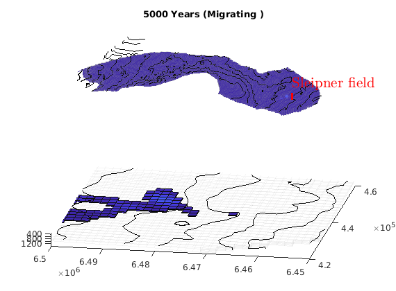
migrateInjection(Gt, traps, petrodata, wellCell, varargin)¶

Run a simple injection scenario and visualize each time step

Synopsis:

function sol = migrateInjection(Gt, traps, petrodata, wellCell, varargin)

DESCRIPTION:

This script runs a simple injection scenario based on a top-surface grid and a single injector well located in a specified grid cell. The simulation uses an incompressible fluid with linear relative permeabilities and sharp interface. Rock is incompressible and homogeneous, with permeability and porosity provided by the ‘petrodata’ argument. After computation of a timestep, the variously trapped volumes are computed, and the result is visualized (either using ‘plotPanelVE’, or simply by using ‘plotCellData’).

For the simulation, pressure is solved using two-point flux approximation. Saturations are computed using implicit transport.

Parameters:

Gt – Top surface grid
traps – trapping structure object, as returned by a call to ‘findTrappingStructure’. Only used for visualizations involving plotPanelVE. Can be left empty, in which case it will be computed internally if needed.
petrodata – structure with the fields ‘avgperm’ (average permeability) and ‘avgporo’ (average porosity). These are single scalars, which will be attributed uniformly to all cells.
wellCell – Index of the cell containing the injection well.
varargin – Allows special options to be set / defaults to be overridden. For instance, the default injection and migration times can be changed, as well as the number of timesteps.

Returns:

sol – simulation solution for the last timestep
report – struct reporting the CPU time for the splitting steps

See also

getAlasGrid

convertAtlasToStruct(meta_thick, meta_top, data_thick, data_top)¶

Create GRDECL struct from thickness/top data from the CO2 Storage Atlas

Synopsis:

grdecl = convertAtlasTo3D(m_thick, m_top, d_thick, d_top, 3)

Description:

Given two datasets with possibily non-matching nodes, interpolate and combine to form a GRDECL struct suitable for 3D simulations after a call to processGRDECL or for further manipulation.

Parameters:	meta_thick – Metainformation for the thickness data as produced from readAAIGrid meta_top – Metainformation for top data. data_thick – Data for the thickness data as produced from readAAIGrid top_thick – Data for the top data as produced from readAAIGrid
Returns:	sqform – GRDECL struct suitable for processGRDECL

Notes

It is likely easier to use getAtlasGrid instead of calling this routine directly.

See also

getAlasGrid

getAtlasGrid(varargin)¶

Get GRDECL grids and datasets for CO2 Atlas datasets

Synopsis:

getAtlasGrid();    % lists all possible datasets

[grdecls datasets petroinfo] = getAtlasGrid();
[grdecls datasets petroinfo] = getAtlasGrid({'Johansenfm', 'Brynefm'});
[grdecls datasets petroinfo] = getAtlasGrid('Johansenfm');

[grdecls ...] = getAtlasGrid(pn1, pv1, ..)
[grdecls ...] = getAtlasGrid('Johansenfm', pn1, pv1, ...)
[grdecls ...] = getAtlasGrid({'Johansenfm', ..}, pn1, pv1, ...)

Parameters:

'pn'/pv –

List of optional property names/property values:

coarsening: Coarsening factor. If set to one, a grid with approximately

one cell per datapoint is produced. If set to two, every second datapoint in x and y direction is used, giving a reduction to 1/4th size. Default: 1

refining: Refining factor. If set to an integer n > 1, each

original cell is laterally split up into n x n cells.

nz: Vertical / k-direction number of layers. Default: 1
make_deck: Boolean. If set to true, the routine will create cell

arrays of data members in ECLIPSE grid structures to represent the 3D grid. If false, the routine will create a structure that contains node points, depth of top surface, thickness of formation, etc.

Note

If called without parameters, the function will list all files in the data directory.

Returns:

grdecls – Cell arrays of data members in ECLIPSE grid structures suitable for processGRDECL if ‘make_deck’ is true. Otherwise, a data structure that contains arrays giving the nodes, depth of top surface, thickness of formation, etc.
datasets – (OPTIONAL) raw datasets used to produce GRDECL structs.
petroinfo – (OPTIONAL) average perm / porosity as given in the atlas. Will contain NaN where values are not provided or possible to calculate.

See also

convertAtlasTo3D, downloadDataSets

getBarentsSeaNames()¶

Returns the formation names present in the Barents Sea.

Note: Sto, Nordmela, and Tubaen formations make up the Hammerfest Aquifer.

According to the Compiled CO2 Atlas, Knurr and Fruholmen formations are not evaluated as an aquifer for CO2 storage or a large injection potential, respectively.

getNorthSeaNames()¶: Returns the formation names present in the North Sea.

getNorwegianSeaNames()¶

Returns the formation names present in the Norwegian Sea.

According to the Compiled CO2 Atlas, Not and Ror are sealing formations and are not evaluated as an aquifer for CO2 storage or a large injection potential, respectively.

processAAIGrid(meta, data, topgrid, cstrids)¶

Process aii grid meta data to a grid .. rubric:: Synopsis:

G = processAAIGrid(meta, data, topgrid, cstrids)

Parameters:	G – Grid data structure. meta – meta data of the grid data – data defining height of surface topgrid – if true make topsurface grid cstrids – stride to make coarser representation
Returns:	G – valid MRST grid. If ‘topgrid’ is true, G has the format of a top-surface grid. If not, G is a 2D grid embedded in 3D

readAAIGrid(filename)¶

Read AIIGrid from file.

Synopsis:

[meta, data] = readAAIGrid('~/testfile')

Parameters:	inp – A valid filename for fopen.
Returns:	meta – metadata defining global coordinate system, cell size, etc. data – A matrix containing the data from the file.

See also

trapAnalysis, showTrappingStructure

updateWithHeterogeneity(deck, petroinfo, meta_top, opt)¶

Update deck and petroinfo to include heterogeneous rock properties

Synopsis:

[deck, petroinfo] = updateWithHeterogeneity( deck, petroinfo, meta_top, opt);

Description:

The CO2Atlas directory is searched and any heterogeneous rock data that exists for a formation matching deck.name is loaded and added to the deck structure. If no rock data files for a formation matching deck.name exist, deck and petroinfo are returned from function unchanged.

Parameters:

deck – cell arrays of data members in ECLIPSE grid structures.
petroinfo – average perm / porosity as given in the atlas. Will contain NaN where values are not provided or possible to calculate.
meta_top – Metainformation for top data, as returned by readAtlasGrids(), a local function in getAtlasGrid()

Returns:

deck – updated cell arrays of data members in ECLIPSE grid structures. If heterogeneous rock properties are available for a formation, these are added to deck structure. If not, deck is returned unmodified.
petroinfo – heterogeneous rock properties and updated average perm / porosity computed from these heterogeneous properties. If no heterogeneous data is available for a formation, petroinfo is returned unmodified.

See also

getAtlasGrid, convertAtlasTo3D

Contents¶

CO2PROPS

Files: addSampledFluidProperties - Add density, viscosity or enthalpy properties to a fluid object. The boCO2 - CO2 formation volume factor function CO2CriticalPoint - Values from paper by Span % Wagner CO2props - Generate a set of CO2 property functions based on sampled data. CO2VaporPressure - Compute the CO2 vapor pressure for a given temperature generatePropsTable - Generates and saves a sampled table of fluid properties, using ‘coolprops’. propFilename - Standardized filename generator for a sampled table of a given property of SampledProp2D - Create a structure with functions to interpolate a 2D sampled property and its

CO2CriticalPoint()¶: Values from paper by Span % Wagner

CO2VaporPressure(T)¶: Compute the CO2 vapor pressure for a given temperature Based on formula 3.13 (p. 1524) of the paper: “A new Equation of State for Carbon Dioxide […]” by Span and Wagner

CO2props(varargin)¶

Generate a set of CO2 property functions based on sampled data.

Synopsis:

function obj = CO2props(varargin)

Description:

Generates a structure containing a number of member functions representing CO2 density, viscosity and enthalpy in terms of pressure and temperature. Derivative functions (and optionally, higher derivatives) are also provided. The functions are computed using sampled tables (which can be changed), and support automatic differentiation as provided within the MRST framework.

Parameters:	are no required parameters. A number of optional parameters can be (There) – as key/value pairs on the form (specified) – include –

:param : rhofile - location of sampled table with density values. The default: table covers the pressure/temperature range [0.1, 400] MPa, [278, 524] K. (400 x 400 samples).
:param : mufile - location of sampled table with viscosity values. The default: table covers the pressure/temperature range [0.1, 400] MPa, [278, 524] K. (400 x 400 samples).
:param : hfile - location of sampled table with enthalpy values. The default: table covers the pressure/temperature range [0.1, 400] MPa, [278, 524] K. (400 x 400 samples).
:param : const_derivatives - true or false. If ‘true’, only first-order: derivative functions will be included.
:param : assert - if ‘true’, a property function will throw an error if user: tries to extrapolate outside the pressure/temperature range covered by the corresponding sampled table. If ‘false’, either NaN values or extrapolated values will be returned in this case, depending on whether the optional parameter ‘nan_outside_range’ is set to ‘true’ or ‘false’.

:param : nan_outside_range - See documentation of ‘assert’ option above. :param : sharp_phase_boundary - If ‘true’, will use one-sided evaluation of

derivatives near the liquid-vapor boundary, in order to avoid smearing or the derivatives across this discontinuity. Useful for plotting, but in general not recommended for simulation code using automatic differentiation, since the discontinuous derivatives may prevent the nonlinear solver from converging.

Returns:	obj – Object containing a full set of CO2 property functions.

See also

SampledProp2D

SampledProp2D(name, file, varargin)¶

Create a structure with functions to interpolate a 2D sampled property and its derivatives, optionally with a discontinuity (phase boundary)

Synopsis:

function res = SampledProp2D(name, file, varargin)

DESCRIPTION:

Parameters:

name – name of property (e.g. ‘density’, ‘viscosity’, ‘rho’, …)
file –
filename containing the sampled values as MATLAB objects. The objects should be: * A 2D matrix named ‘vals’, representing the actual sampled

values
- Two structs, representing the two variables for which the table has been sampled. The structs contain the fields: - num - number of sample points for this variable - span - vector with 2 components, representing the range
  
  of the variable
  - stepsize - the size of each step. Should equal diff(span)/num.
varargin –
optional parameters (as key/value pairs) are: - ‘assert_in_range’: If ‘true’, throw an error if user tried

to extrapolate outside valid range.
- ’nan_outside_range’: If ‘true’ (default), return NaN
  
  values outside valid range. Otherwise, extrapolate as constant function.
- ’phase_boundary’: Cell array. If nonempty, the first
  
  cell contains the parameter values for the critical point (start of the discontinuity line). The second cell contains a function that describes the dicontinuity line as a relation between the two variables, on the form v2 = f(v1).
- ’const_derivatives’: If ‘true’ (default), only first-order
  
  partial derivatives are included. Otherwise, second-order partial derivatives are included as well. For code based on automatic differentiation, it is recommended to avoid the second-order partial derivatives.

Returns:

res – Struct containing the generated functions.

addSampledFluidProperties(fluid, shortname, varargin)¶

Add density, viscosity or enthalpy properties to a fluid object. The properties may be those of CO2 or of water.

Synopsis:

function fluid = addSampledFluidProperties(fluid, shortname, varargin)

Description:

This function endows a preexisting fluid object with property functions for density, viscosity and/or enthalpy. These functions will depend on pressure and temperature, or on pressure only (if requested), and are computed based on sampled tables.

Parameters:

fluid – Preexisting fluid object to receive the requested property functions.
shortname – Either ‘G’ (for gas, i.e. CO2 property functions) or ‘W’, for water property functions.
varargin –
Optional arguments supplied as ‘key’/value pairs (‘pn’/nv). These include:
- pspan - 2-component vector [pmin pmax] to specify the upper
  
  and lower pressure range (Pa) of the sampled table. If no such table preexists, it will be computed using the CoolProps software package (if this is not available, an error will be thrown).
- tspan - 2-component vector [tmin tmax] to specify the upper
  
  and lower temperature range (K) of the sampled table. If no such table preexists, it will be computed using the CoolProps software package (if this is not available, an error will be thrown).
- pnum - number of (equidistant) samples along the pressure
  
  dimension in the sampled table.
- tnum - number of (equidistant) samples along the
  
  temperature dimension in the sampled table.
- props - 4-component logical vector (true/false) indicating
  
  which property functions to include, on the form: [density, viscosity, enthalpy, conductivity]
- fixedT - If empty (default), the returned properties will be
  
  functions of pressure AND temperature. If ‘fixedT’ is a value (or vector of values), the returned properties will be functions of pressure only, with temperature consided constant and equal to the value(s) provided in ‘fixedT’.
- ’assert_in_range’: If ‘true’, throw an error if user tried
  
  to extrapolate outside valid range. If ‘false’ (default), behavior in this case will depend on the value of ‘nan_outside_range’.
- ’nan_outside_range’: If ‘true’ (default), return NaN
  
  values outside valid range. Otherwise, extrapolate as constant function.
- ’include_derivatives’: include explicit functions for
  
  partial derivatives in pressure and temperature (default: false)

Returns:

fluid – Fluid object endowed with the property functions (or a subset
thereof) – rhoG, rhoW, muG, muW, hG, hW.

boCO2(T_ref, rhoG, varargin)¶

CO2 formation volume factor function

Synopsis:

function bG = boCO2(T_ref, rhoG, varargin)

Description:

Produces a function representing the CO2 formation volume factor, which expresses the density of CO2 as a fraction of some reference (surface) density. The returned function depends on pressure only (reference temperature to be used is provided in the function call.

Parameters:

T_ref – Reference temperature to be used (since the returned function should only depend on pressure). Since the reference temperature may vary across the grid (due to a spatially dependent temperature field, ‘T_ref’ can be given as a vector of values.
rhoG – Reference density
varargin –
Optional parameters can be specified as key/value pairs on the
form (‘key’/value …). These include:
- rho_datafile - name of datafile containing the sampled table to
  
  be used for computing CO2 densities as functions of pressure and temperature.
- sharp_phase_boundary - If ‘true’, will use one-sided evaluation
  
  of derivatives near the liquid-vapor boundary, in order to avoid smearing or the derivatives across this discontinuity. Useful for plotting, but in general not recommended for simulation code using automatic differentiation, since the discontinuous derivatives may prevent the nonlinear solver from converging.

Returns:

bG – CO2 formation volume factor (a function of pressure)

See also

CO2props, SampledProp2D

generatePropsTable(savedir, fluidname, pname, P_range, T_range, P_num, T_num)¶

Generates and saves a sampled table of fluid properties, using ‘coolprops’.

NB: ‘coolprops’ needs to be available, which means that the directory containing the function ‘propsSI’ needs to be in the search path, and the corresponding mex-files must be compiled and available

Synopsis:

function tables = generatePropsTable(fluidname, pname, P_range, T_range, P_num, T_num)

DESCRIPTION:

Parameters:

fluidname – name of fluid. should be ‘Carbon dioxide’ or ‘Water’
pname – property name. ‘D’ for density; ‘V’ for viscosity or ‘H’ for enthalpy
P_range – [pmin, pmax] : lower and upper end of sampled pressure range (Pascal)
T_range – [tmin, tmax] : lower and upper end of sampled temp. range (Kelvin)
P_num – number of (evenly spaced) pressure samples within ‘P_range’
T_num – number of (evenly spaced) temperature samples within ‘T_range’

Returns:

Nothing. The generated table is saved directly, along with the – information on pressure and temperature ranges.

propFilename(P_range, T_range, P_num, T_num, fluid, prop)¶: Standardized filename generator for a sampled table of a given property of a given fluid, with given sample parameters.

Contents¶

GRID

Files: boundaryCellsSubGrid - Compute set of cells on the boundary of a subgrid boundaryFaceIndices - Retrieve face indices belonging to subset of global outer faces. computeGeometryVE_2D - Compute geometry of grid of top-surface grid so that the geometry is mapAxes - Transform lateral position from map to local coordinate system topSurfaceGrid - Make a hybrid grid of the top surface of a 3D grid having a logical

boundaryCellsSubGrid(G, c, varargin)¶

Compute set of cells on the boundary of a subgrid

Synopsis:

bc = boundaryCellsSubGrid(G, c)

Parameters:	G – Grid structure. c – List or logical mask of cells constituting a subgrid of ‘G’. ’pn’/pv - List of ‘key’/value pairs defining optional parameters. The supported options are: neigbours - use other neibours than in grid
Returns:	bc – List of cell indices that constitute the boundary cells of the subgrid.

boundaryFaceIndices(G, direction, i1, i2, i3)¶

Retrieve face indices belonging to subset of global outer faces.

Synopsis:

ix = boundaryFaceIndices(G, side, i1, i2, i3)

Parameters:

G – Grid data structure.
side –
Global side from which to extract face indices. String. Must (case insensitively) match one of six alias groups:
1. {‘West’ , ‘XMin’, ‘Left’ }
2. {‘East’ , ‘XMax’, ‘Right’ }
3. {‘South’, ‘YMin’, ‘Back’ }
4. {‘North’, ‘YMax’, ‘Front’ }
5. {‘Upper’, ‘ZMin’, ‘Top’ }
6. {‘Lower’, ‘ZMax’, ‘Bottom’}
These groups correspond to the cardinal directions mentioned as the first alternative in each group.
i1,i2,i3 – Index ranges in which one is to look for boundary faces in the three axial directions

Returns:

ix – Required face indices.

Note

This function is mainly intended for internal use by functions fluxside and pside. Its calling interface may change more frequently than those of the *side functions.

See also

fluxside, pside.

computeGeometryVE_2D(Gt, varargin)¶

Compute geometry of grid of top-surface grid so that the geometry is defined by its projection and the z value is the value at face corresponting to the top of the column

Synopsis:

Gt = computeGeometryVE(Gt)
Gt = computeGeometryVE(Gt, varargin)

Parameters:

Gt – Grid structure as defined by function ‘topSurfaceGrid’. Gt.parent is the original grid
'pn'/pv –
List of ‘key’/value pairs for supplying optional parameters. The supported options are
- Verbose – Whether or not to display verbose output as
  
  the process progresses. Possible values are TRUE and FALSE. Default value equals mrstVerbose.

Returns:

Gt – Grid structure with added fields: - cells

volumes

centroids

z

faces
- areas
- normals !!! AREA WEIGHTED !!!
- centroids
- z

mapAxes(pos, MA)¶

Transform lateral position from map to local coordinate system

Synopsis:

p = mapAxis(pos, ma)

Parameters:	pos – nx2 vector of map coordinates that are to be transformed ma – 6x1 vector of points: x1 y1 x2 y2 x3 y3 Here: (x1,y1) describes a point on the y-axis, (x2,y2) is the grid origin, and (x3,y3) is a point on the x-axis
Returns:	p – nx2 vector of coordinates transformed to local coordinate system

Example:

p = mapAxes([x y], [100 100 0 100 100 0])

topSurfaceGrid(G)¶

Make a hybrid grid of the top surface of a 3D grid having a logical ijk-index (e.g., a corner-point grid or a logically Cartesian grid)

SYNOPSIS:

[Gt,G] = topSurfaceGrid(G)

PARAMETERS:

G - 3D grid as described by grid_structure.

RETURNS:

Gt - structure representing the top-surface grid. The structure

consists of two parts:

the surface projected onto the xy-plane represented as a standard 2D grid that follows the standard grid conventions as outlined in grid_structure,

a set of extra fields that represent the surface elevation, the

3D surface normals, the elevation of the bottom surface, the height of the surface, the columns of volumetric cells attached to each cell (quadrilateral patch) in the 2D grid, etc.

Altogether, the hybrid grid structure contains the following fields:

cells – A structure specifying properties for each individual

cell in the grid. See CELLS below for details.

faces – A structure specifying properties for each individual

face in the grid. See FACES below for details.

nodes – A structure specifying properties for each individual

node (vertex) in the grid. See NODES below for details.

columns – A structure specifying properties of each individual

vertically-averaged column. See COLUMNS below for details.

type – A cell array of strings describing the history of grid

constructor and modifier functions through which this particular grid has been defined.

G - 3D grid with connected columns and no disconnected cells,

corresponding to Gt. Important to use this 3D grid when doing comparisons or if 2D data is mapped back to 3D grid.

FIELDS in a 2D top-surface grid:

COLUMNS - Cell structure Gt.columns that represents the column of cells in the 3D grid that are attached to each cell in the top-surface grid. Containts the fields:

cells – A G.cells.num-by-1 array of cell indices from the

3D grid, which together with Gt.cells.columnPos define the columns attached to the top surface.

dz – A G.cells.num-by-1 array of heights of the cells in the

3D grid defined as the vertical difference between the centroids of the top and bottom surfaces of each cell (faces labelled 5 and 6).

z – A G.cells.num-by-1 array of the z-component of the

centroid of the bottom surface of each cell, defined relative to the height of the centroid of the top surface, i.e., a column-wise cumsum of columns.dz.

CELLS - Cell structure Gt.cells, as described by grid_structure but with the extra fields:

columnPos – Indirection map of size [num+1,1] into the

‘columns.cells’ array. Specifically, the cells in the column of the 3D grid corresponding to cell ‘i’ in the top-surface grid are found in the submatrix

Gt.columns.cells(columnPos(i):columnPos(i+1)-1,:)

The number of cells in the each column can be computed by the statement DIFF(columnPos)

map3DFace – A cells.num-by-1 array that maps between a cell in the

top-surface grid and the corresponding top face in the underlying 3D grid, i.e., cell ‘i’ corresponds to face number Gt.cells.map3DFace(i).

ij – A map of size [num,1] giving logical indices of the

cells in the top-surface grid

H – A array of formation heights, one for each cell

normals – normal vector of the surface represented by each cell

z – A cells.num-by-1 array of the third coordinate of the

cell centroids in R^3. The first two coordinates are given in Gt.cells.

grav_pressure and primitives

– these two fields are necessary when solving the system

sequentially using “solveIncompFlow” with an s-formulation.

FACES - Cell structure Gt.faces, as described in grid_structure but with the following extra field created by a subsequent call to computeGeometryVE:

z – A faces.num-by-1 array of the third coordinate of the

face centroids in R^3. The first two coordinates are given in Gt.faces.centroids.

NODES - Cell structure Gt.nodes, as described in grid_structure but with the following extra field created by a subsequent call to computeGeometryVE:

z – A nodes.num-by-1 array of the third coordinate of the

node positions in R^3, i.e., the z-coordinate of the top surface of the original grid. The first two coordinates are given in Gt.nodes.coords.

COMMENTS:

PLEASE NOTE: The current implementation does not honour faults and internal boundaries from 3D grid, i.e., it is possible to get false connections over faults if there is no jump in the ij index over the fault in the 3D grid.

Contents¶

MAPPINGS

Files: accumulateVertically - Accumulate quantity vertically per column. cumulativeHeight - Compute cumulative height for each column. cumulativePoreHeight - Compute cumulative pore height for each column. fillDegree - Compute degree of fill (saturation). height2Sat - Convert from height to saturation integrateVertically - Compute integral of function, vertically per column. invertVerticalFunction - Solve y(z)=f for piecewise linear, monotonically increasing function y. normalizeValuesVE - Normalizes values for different VE grids and formulations. sat2height - Convert from saturation to height upscaledSat2height - Compute upscaled height, based on upscaled saturation

accumulateVertically(q, p)¶

Accumulate quantity vertically per column.

Synopsis:

cq = accumulateVertically(q, pos)

Parameters:	q – Sampled quantity values. One scalar value for each cell in each column. pos – Column indirection array. Specifically, pos(i) : pos(i + 1) - 1 are the indices in ‘q’ which correspond to column ‘i’.
Returns:	cq – Accumulated ‘q’ values. Corresponds to CUMSUM(q), but reset per column such that ALL(cq(pos(1 : end-1)) == 0).

See also

topSurfaceGrid, cumsum.

cumulativeHeight(g)¶

Compute cumulative height for each column.

Synopsis:

z = cumulativeHeight(G)

Parameters:

G – A top-surface grid as defined by function ‘topSurfaceGrid’.

Returns:

z –

A G.cells.num-by-1 array of doubles such that

z(G.columns.pos(i) : G.columns.pos(i+1)-1))

contains the cumulative height, measured from top-level z==0, of the bottom interface of each 3D cell in column ‘i’. Specifically, when

p = G.columns.pos(1 : end-1),

then

z(p) == G.columns.dz(p)

modulo arithmetic error (round-off).

cumulativePoreHeight(g, rock)¶

Compute cumulative pore height for each column.

Synopsis:

ph = cumulativePoreHeight(G, rock)

Description:

Define the pore height of a cell c as dz(c)*phi(c).

Parameters:

G – A top-surface grid as defined by function ‘topSurfaceGrid’.
rock – Rock data structure. Must contain valid field ‘rock.poro’.

Returns:

pI –

A G.cells.num-by-1 array of doubles such that

pv(G.cells.columnPos(i) : G.cells.columnPos(i+1)-1))

contains the cumulative pore height, measured from top-level z==0, at the bottom interface of each 3D cell in column ‘i’.

Note

This function is to the pore height what function cumulativeHeight is to the incremental depth, G.columns.dz.

fillDegree(h, G)¶

Compute degree of fill (saturation).

Synopsis:

[n, t] = fillDegree(h, G)

Parameters:

h –
CO2 plume thickness. One scalar value for each column in the top-surface grid. As a special case a single, scalar value is repeated for each column in the top-surface grid.

Values less than zero are treated as zero while values below the bottom of a column are treated as the column depth.
G – A top-surface grid as defined by function ‘topSurfaceGrid’.

Returns:

n – Number of completely filled cells. One non-negative integer for each grid column. If the top-most cell in column ‘i’ is partially filled, then n(i)==0.
t – Fill degree of column’s single partially filled cell. One scalar value between zero and one (inclusive, i.e., t in [0,1]) for each column. If a column is completely filled (i.e., if n(i) equals the number of cells in column ‘i’), then t(i) is (arbitrarily) set to zero.

Note

Assume column ‘i’ consists of N(i) cells. Then, implicitly, the saturation is s==1 in the n(i) first cells of this column. Furthermore, s=t(i) in cell n(i)+1, and s==0 in the remaining N(i) - (n(i) + 1) cells below the single, partially filled cell.

height2Sat(sol, Gt, fluid)¶

Convert from height to saturation

Synopsis:

s = height2Sat(sol, Gt, fluid)

Parameters:	h – CO2 plume thickness. One scalar value for each column in the top-surface grid. Values less than zero are treated as zero while values below the bottom of a column are treated as the column depth. Gt – A top-surface grid as defined by function ‘topSurfaceGrid’. fluid – a fluid object for example initiated with initVEFluid
Returns:	s – Saturation - one value for each cell in the underlying 3D model. Corresponds to state.s for the 3D problem.

integrateVertically(fun, h, g)¶

Compute integral of function, vertically per column.

Synopsis:

F = integrateVertically(f, h, G)

Description:

Computes a first order approximation to the integral

F(x,y) = int_0^h f(x,y,z) dz

within each column of a top-surface grid.

Parameters:

fun – Sampled values of function f(x,y,z). One value for each cell in the underlying three-dimensional model.
h – Upper bound for the integral (*). Typically corresponds to the surface depth. One scalar value for each column in the top-surface grid. As a special case a single, scalar value is repeated for each column in the top-surface grid.
G – A top-surface grid as defined by function ‘topSurfaceGrid’.

Returns:

F – Vertically averaged function value, F(x,y). One scalar value for each column in the top-surface grid ‘G’.

See also

topSurfaceGrid, cumulativeHeight.

invertVerticalFunction(f, g, z, y)¶

Solve y(z)=f for piecewise linear, monotonically increasing function y.

Synopsis:

h = invertVerticalFunction(f, G, z, y)

Parameters:

f – Specific function values of the function y=y(z). One scalar value for each column in the top-surface grid. As a special case, a single, scalar value is repeated for each column in the grid.
G – A top-surface grid as defined by function ‘topSurfaceGrid’.
z – Sample points (typically column depths) for the function y=y(z). Possibly computed by means of function ‘cumulativeHeight’.
y – Sampled values of the function y=y(z) at the points ‘z’. Often corresponds to cumulative pore height as defined by function ‘cumulativePoreHeight’.

Returns:

h – Depth values (z) such that y(z)=f in each column. One scalar value for each column.

Example:

% Define geometry and rock data.
grdecl    = makeModel3([100, 60, 15]);
G         = computeGeometry(processGRDECL(grdecl));
G         = topSurfaceGrid(G);
rock.poro = rand([numel(G.columns.cells), 1]);        % Synthetic...

% Compute cumulative column depths and pore heights.
z  = cumulativeHeight(G);
ph = cumulativePoreHeight(G, rock);

% Compute depth (h) of 0.5 (total) column pore height.
f = 0.5 * ph(G.cells.columnPos(2 : end) - 1);
h = invertVerticalFunction(f, G, z, ph);

% Plot depth map of 0.5 pore height as a fraction of the
% corresponding (total) column depth.
plotCellData(G, h ./ z(G.cells.columnPos(2:end) - 1))
caxis([0, 1]); colorbar

Note

The function y=y(z) is assumed to be a piecewise linear, monotonically increasing function (per column) satisfying y(0)=0.

normalizeValuesVE(g_top, sol, fluid, varargin)¶

Normalizes values for different VE grids and formulations.

Synopsis:

[s h hmax]  = normalizeValuesVE(g_top, sol, fluid)
[s h hmax]  = normalizeValuesVE(g_top, sol, fluid, 'CoupledGrid', g_coupled)

Parameters:

g_top – top surface 2D grid as defined by function ‘topSurfaceGrid’.
sol – Reservoir solution from for example initResSol
fluid – A valid fluid object for the formulation
'pn'/pv –
List of ‘key’/value pairs defining optional parameters. Supported options are:

’CoupledGrid’ – The coupled grid. Needed if using a coupled formulation. ‘Rock’ – fine scale rock structure for coupled h calculations using sat2height

Returns:

s – Fine scale saturation based on the values. This will be suitable for plotting with the full 3D grid the top surface grid was made from.
h – Height values suitable for plotting with the top surface grid. Contains g_top.cells.num elements.

sat2height(s, g, rock)¶

Convert from saturation to height

Synopsis:

h = sat2height(s, G, rock)

Parameters:	s – Saturation - one value for each cell in the underlying 3D model. Corresponds to state.s for the 3D problem. G – A top-surface grid as defined by function ‘topSurfaceGrid’. rock – 3D rock data containing valid filed ‘poro’.
Returns:	h – Plume thickness. One scalar value for each column in the top-surface grid.

upscaledSat2height(S, S_max, Gt, varargin)¶

Compute upscaled height, based on upscaled saturation

Synopsis:

function [h, h_max] = upscaledSat2height(S, S_max, varargin)

DESCRIPTION: Compute upscaled height (present and max), based on upscaled saturation (present and max), based either on a sharp-interface model, or a general model where the upscaled capillary pressure function is provided by the caller.

Parameters:

S – Upscaled present saturation
S_max – Upscaled, historically maximum, saturation
Gt – Top-surface grid in question
varargin –
Additional parameters (key, value), depending of conversion model: * If a _sharp interface model_ (with vertically constant rock properties) is assumed, then the function needs the following argument:
- ’resSat’ - [rw, rc], where ‘rw’ is the residual water
  
  saturation (assumed constant), and ‘rc’ is the residual CO2 saturation.
- If a _general_ model is assumed, then the function needs the
following argument:
- pcWG(S, p, S_max) - upscaled capillary pressure as a
  
  function of upscaled saturation, current pressure and max. upscaled saturation.
- rhoW(p) - density of water [oil] phase, as a
  
  function of pressure.
- rhoG(p) - density of CO2 [gas] phase, as a
  
  function of pressure.
- ’p’ - current pressure (Upscaled capillary pressure here defined as the pressure difference between phases at the level of the caprock, assuming that the difference is 0 at depth ‘h’ (the deepest point where there is free flow of CO2).

Returns:

h – The height, corresponding to the vertical distance between caprock and the deepest point for which there is still nonzero CO2 flow.
h_max – The historically maximum height

Contents¶

MISC

Files: moduleCheck - Load specified modules unless already active userConsent - userConsent Ask user for his/her consent to a Y/N question VEROOTDIR - Retrieve full path of VE-root directory.

VEROOTDIR()¶

Retrieve full path of VE-root directory.

Synopsis:

veroot = VEROOTDIR

Parameters:	none. –
Returns:	veroot – Full path to VE module installation directory.

moduleCheck(varargin)¶

Load specified modules unless already active

Synopsis:

moduleCheck m1 [m2 ...]

PARAMETERS

m1, … - Module names. Must be known in mrstPath. If a module is not: alread active, the module will be loaded through mrstModule.

Returns:	Nothing.

Note

Use functional form of moduleCheck if the module name string is contained in a variable.

See also

mrstPath, mrstModule.

userConsent(question)¶

userConsent Ask user for his/her consent to a Y/N question c = userConsent(question) requests a text response from the user in the form of a Y/N question. The function returns logical 1 (true) if the the first letter in the user’s response is a ‘y’ (or ‘Y’), and returns logical 0 otherwise. Default answer is ‘Y’.

Example: userConsent(‘Do you want to continue’) will produce the following prompt “Do you want to continue? Y/N [Y]: “

Contents¶

OPTIMIZATION

Files: computeToptraps - Compute subscale trapping potential for all cells in a top surface grid, optimizeControls - Compute an optimal set of well controls (‘rate’ or ‘bhp’) for a proposed optimizeFormation - Optimize a injection scenario for a formation from the CO2-atlas. Well optimizeRatesIPOPT - Compute an optimal set of injection rates for a proposed setSchedule - Construct a schedule object that is convenient for use with

computeToptraps(trapfun, Gt, recenter)¶

Compute subscale trapping potential for all cells in a top surface grid, based on a precomputed trap function.

Synopsis:

function dh = computeToptraps(trapfun, Gt, recenter)

DESCRIPTION:

Parameters:	trapfun – precomputed trap function (As computed by e.g. ‘resTiltUtsira.m’) Gt – top surface grid recenter – whether or not to ‘recenter’, i.e. adjust angle so that maximum subscale trapping is obtained when surface is horizontal
Returns:	dh – vector with one entry per cell of ‘Gt’, giving the subscale trapping potential for each cell.

See also

resTiltUtsira

optimizeControls(initState, model, schedule, min_wvals, max_wvals, varargin)¶

Compute an optimal set of well controls (‘rate’ or ‘bhp’) for a proposed injection/migration scenario.

Synopsis:

function [optim, init, history] = ...
   optimizeControls(initState, model, schedule, min_wvals, max_wvals, varargin)

Description:

The injection phase can consist of multiple control periods. If a migration phase is included, it must be only one control period, and it must be the last control period. Individual wells must be of the same well type (either ‘rate’ or ‘bhp’) during the entire injection phase. If there’s a migration phase, all wells must be of well type ‘rate’. Individual well signs must remain fixed over all periods (+1 for injector, -1 for producer).

Parameters:

initState – initial state
model – simulation model (instance of CO2VEBlackOilTypeModel)
schedule – initial proposed injection schedule (which also includes information on the placement of wells)
min_wvals – minimum allowed well control values during injection phase
max_wvals – maximum allowed well control values during injection phase
varargin –
An optional number of paired arguments on the form: ‘option’, value. Possible options are: - dryrun: if ‘true’, no optimization will take place (only

the associated data structures will be set up)
- obj_scaling: scaling factor of the objective function (if
  
  left empty, will be computed internally)
- leak_penalty: penalty leak factor (default: 10)
- last_control_is_migration: (true or false)
  
  if ‘true’, the last control will be constrained to zero rate (assumed to represent the migration phase)
- obj_fun: specify the objective function to maximise. If
  left empty, a default objective function will be used that aims to maximise injected CO2 while minimizing leakage. The objective function, if specified, should take the following arguments: - wellSols: vector of well solutions for all
  
  simulation timesteps
  - states: vector of simulation states for
    
    all timesteps
  - schedule: the injection schedule
  - varargin: optional arguments should support
    
    ’ComputePartials’, and ‘tStep’. If ‘ComputePartials’ is true, computed values will be ADI (automatic differentiation objects).
  The function shall return a cell array containing the objective value for each timestep.

Returns:

optim – Data structure containing all information about the final, optimized scenario (including wells and the optimized schedule).
init – Data structure containing all information about the starting point scenario (before optimization of rates).
history – Information about the rate optimization process

Example:

For an example, refer to the sample script 'optimizeUtsira'.

optimizeFormation(varargin)¶

Optimize a injection scenario for a formation from the CO2-atlas. Well positions are selected based on structural trapping potential, and rates are chosen to maximise storage while minimizing leakage.

Synopsis:

function [Gt, optim, init, history, other] = optimizeFormation(varargin)

Parameters:

varargin –

a number of paired arguments on the form: ‘option’, value. Options include: - modelname: name of the formation (default: ‘utsirafm’) - schedule: proposed initial schedule (leave empty for

automatic specification of schedule with well placement and initial rates based on top surface geometry).

coarse_level: downsampling level of formation grid (to

lower computational cost)
num_wells: desired number of wells (default 10)
subtrap_file: file containing information on estimated

subscale trapping for the given formation (empty for no subscale trapping).
sr: residual CO2 saturation
sw: residual brine saturation
isteps: number of injection timesteps
msteps: number of migration timesteps
itime: total duration of injection phase
mtime: total duration of migration phase
maxmise_boundary_distance (true/false):

if true, wells will be placed as far as possible from boundary within the chosen catchment region
well_buffer_dist:

if ‘maximize_boundary_distance’ is fasle, wells should (if possible) be within this distnace of the relevant spill region’s boundary.
report_basedir: directory for saving results

Returns:

Gt – Top surface grid of the chosen formation
optim – Data structure containing all information about the final, optimized scenario (including wells and the optimized schedule).
init – Data structure containing all information about the starting point scenario (before optimization of rates).
history – Information about the rate optimization process
other – Data structure containing additional information needed to rerun the optimized scenario (fluid and rock objects, residual saturation, trapping structure, subscale trapping, and initial state)

Example:

For an example, refer to the sample script 'optimizeUtsira'.

optimizeRatesIPOPT(initState, model, schedule, min_rates, max_rates, varargin)¶

Compute an optimal set of injection rates for a proposed injection/migration scenario.

Synopsis:

function [optim, init, history] = ...
   optimizeRates(initState, model, schedule, min_rates, max_rates, varargin)

DESCRIPTION:

Parameters:

initState – initial state
model – simulation model (instance of CO2VEBlackOilTypeModel)
schedule – initial proposed injection schedule (which also includes information on the placement of wells)
min_rates – minimum allowed rates
max_rates – maximum allowed rates
varargin –
An optional number of paired arguments on the form: ‘option’, value. Possible options are: - dryrun: if ‘true’, no optimization will take place (only

the associated data structures will be set up)
- obj_scaling: scaling factor of the objective function (if
  
  left empty, will be computed internally)
- leak_penalty: penalty leak factor (default: 10)
- last_control_is_migration: (true or false)
  
  if ‘true’, the last control will be constrained to zero rate (assumed to represent the migration phase)
- obj_fun: specify the objective function to maximise. If
  left empty, a default objective function will be used that aims to maximise injected CO2 while minimizing leakage. The objective function, if specified, should take the following arguments: - wellSols: vector of well solutions for all
  
  simulation timesteps
  - states: vector of simulation states for
    
    all timesteps
  - schedule: the injection schedule
  - varargin: optional arguments should support
    
    ’ComputePartials’, and ‘tStep’. If ‘ComputePartials’ is true, computed values will be ADI (automatic differentiation objects).
  The function shall return a cell array containing the objective value for each timestep.

Returns:

optim – Data structure containing all information about the final, optimized scenario (including wells and the optimized schedule).
init – Data structure containing all information about the starting point scenario (before optimization of rates).
history – Information about the rate optimization process

Example:

For an example, refer to the sample script 'optimizeUtsira'.

setSchedule(Gt, rock, wcells, qtot, isteps, itime, msteps, mtime, single_control, varargin)¶

Construct a schedule object that is convenient for use with ‘optimizeFormation’. Wells are rate-controlled.

SYNOPSIS: function schedule = setSchedule(Gt, rock, wcells, qtot, isteps, itime, …

msteps,mtime, single_control, varargin)

Parameters:

Gt – the simulation grid (top surface grid)
rock – associated rock structure
wcells – well cells (vector containing the indices of the well cells, one entry per welll)
qtot – total amount to inject into each well (vector with one entry per well). Rates will be obtained by dividing entries of this vector by total injection time.
isteps – number of injection time steps
itime – duration of injection phase
msteps – number of migration time steps
mtime – duration of migration phase
single_control – whether the injection phase should be governed by one single control, or a new control for each timestep (allowing for dynamic adjustment of rates)
varargin – The only optional argument is ‘minval’, which specifies the minimum possible rate for a well.

Returns:

schedule – the constructed schedule

See also

optimizeFormation

Contents¶

PLOTTING

Files: getInventoryColors - Return colors used for plotting CO2 inventories (green to orange color) getVEColors - Return colors used for plotting VE models plotPanelVE - Make a panel plot used in the examples of the VE module plotPlume - Plot CO2 plume on logically Cartesian grid plotTrappingDistribution - Generate a trapping inventory plot from a simulation result.

getInventoryColors(ind)¶

Return colors used for plotting CO2 inventories (green to orange color)

Synopsis:

c = getInventoryColors(ind)

Parameters:

ind –

a scalar or vector consisting of one or more of the numbers one to seven. These numbers signify the following parts of a CO2 inventory:

1 - dissolved 2 - residual (traps) 3 - residual 4 - residual (plume) 5 - movable (traps) 6 - movable (plume) 7 - leaked

Returns: c – a numel(ind)x3 vector specifying one RGB color per entry in ‘ind’

Example:

image(repmat(1:7,2,1)); colormap(getInventoryColors(1:7))

See also

interactiveTrapping, getVEColors

getVEColors(ind)¶

Return colors used for plotting VE models

Synopsis:

c = getVEColors(ind)

Parameters:

ind –

a scalar or vector consisting of one or more of the numbers one to five, or a cell array consisting of a set of strings, that signify the following parts of a VE model:

1 - trapped 2 - plume 3 - residual 4 - dissolved 5 - brine

Returns: c – a numel(ind)x3 vector specifying one RGB color per entry in ‘ind’

Example:

image(repmat(1:5,2,1)); colormap(getVEColors(1:5))

See also

getInventoryColors

plotPanelVE(G, Gt, W, sol, t, vol, varargin)¶

Make a panel plot used in the examples of the VE module

SYNOPSIS: plotPanelVE(G, Gt, sol, t, vol) plotPanelVE(G, Gt, sol, t, vol, ‘pn1’, pv1, …)

h = plotPanelVE(…)

Parameters:	G – Grid data structure for 3D grid Gt – Grid data structure for topsurface grid W – Well sol – Solution data structure t – Time vol – Vector of (free, trapped, total) volumes. It will have either four or six entries, as explained below. opt – Various options 'pn'/pv – List of ‘key’/value pairs defining optional parameters.

Description:

The function will make a composit plot that consists of several parts

a 3D plot of the plume
a pie chart of trapped versus free volume
a plane view of the plume from above
two cross-sections in the x/y directions through the well

Supported options for the 3D plot of saturations

‘maxH’ – Double, maximal height value used for scaling the: colorbar. Default value: 10

‘view’ – Vector, view angle. Default value: [30,60] ‘wireS’ – Bool, if true, plot only positive saturation values

on top of a wireframe grid. Default value: false

‘Wadd’ – Double, height added to the well. Default value: 100 ‘Saxis’ – Vector, scaling of caxis. Default value: [0 1]

Supported options for the plot of CO2 height:

‘wireH’ – Bool, if true, plot only positive saturation values: on top of a wireframe grid. Otherwise, make a color plot with height shown as contours. Default value: false
‘ptol’ – Double, smallest number that is considered as positive: in the wireframe plot. Default value: 1e-3

Supported options for the slice plots:

‘slice’ – Vector, index along which to pick the two 2D slices: Default value: slice=[10 10]
‘plotPlume’ – Boolean indicating if the plume should be plotted as: a sharp interface.

Entries ov argument vector ‘vol’:

If only residual trapping (not structural trapping) is considered, ‘vol’ will have four entries, with the following meaning:

vol(1) – residually trapped volume outside the movable zone vol(2) – residually trapped volume within the movable zone vol(3) – free volume (volume of movable zone minus vol(2)) vol(4) – total volume (the others ought to sum up to this one)

If residual trapping and structural trapping are both considered, ‘vol’ will have six entries, with the following meaning (for a more in-depth description, refer to documentation of the function ‘volumesVE’:

vol(1) – vol. of CO2 that is BOTH residually and structurally

trapped

vol(2) – vol. of CO2 that is residually (but not structurally)

trapped, and that is outside the free-flowing zone

vol(3) – vol. of CO2 that is residually (but not structurally)

trapped, and that is still inside the free-flowing zone

vol(4) – vol. of CO2 that is structurally (but not residually)

trapped.

vol(5) – vol. of CO2 that is neither structurally nor residually

trapped.

vol(6) – total volume (the others ought to sum up to this one).

In addition, the function may plot the CO2 inventory as a function of time if the user clicks the pie chart or if the option ‘plotHist’ is set to true.

See also

runIGEMS, volumesVE

plotPlume(G, Gt, h, varargin)¶

Plot CO2 plume on logically Cartesian grid

Synopsis:

 plotPlume(G, Gt, h)
 plotPlume(G, Gt, h, cells)
 plotPlume(G, Gt, h, 'pn1', pv1, ...)
 plotPlume(G, Gt, h, 'pn1', pv1, ...)

h = plotPlume(...)

Parameters:	G – Grid data structure. Gt – Corresponding top grid as defined by topSurfaceGrid h – height dataset for the topSurfaceGrid cells – (OPTIONAL) Cells of G to include in plot. 'pn'/pv – List of other property name/value pairs. OPTIONAL. This list will be passed directly on to function PATCH meaning all properties supported by PATCH are valid.
Returns:	h – Handle to resulting PATCH object. The patch object is added to the current AXES object.

Notes

Function ‘plotPlume’ is implemented directly in terms of the low-level function PATCH. If a separate axes is needed for the graphical output, callers should employ function newplot prior to calling ‘plotPlume’.

See also

plotCellData, plotGrid, newplot, patch, shading.

plotTrappingDistribution(ax, report, varargin)¶

Generate a trapping inventory plot from a simulation result.

The simulation result (set of states) first needs to be repackaged using the ‘makeReports’ function.

Synopsis:

function plotTrappingDistribution(ax, report, varargin)

DESCRIPTION:

Parameters:	ax – handle to figure into which to draw the plot report – simulation results, repackaged using the ‘makeReports’ function varargin – optional argument pairs allowing to specify the location and orientation of the legend.

See also

makeReports.

Contents¶

TRAPPING

Files: downstreamTraps - Return index of all traps downstream of ‘trap_ix’. Also include findOptimalInjectionPoint - Find the optimal point to inject CO2 flattenTraps - Given output res from trapAnalysis, produce a grid with flat top surfaces in trap areas. maximizeTrapping - Find the N best injection trees, with optional compensation for overlap trapAnalysis - Compute and summarize the relevant trap analysis information volumesOfTraps - Compute volumes of (a subset of) precomputed structural traps

downstreamTraps(Gt, poro, tstruct, trap_ix)¶

Return index of all traps downstream of ‘trap_ix’. Also include ‘trap_ix’. If output argument ‘vols’ is provided, the trap volumes will also be computed.

Synopsis:

function [trap_ixs, vols] = downstreamTraps(Gt, poro, tstruct, trap_ix)

Parameters:	Gt – Top surface grid in which the trap lies poro – Porosity field (one value per cell in Gt) tstruct – trap structure og Gt, as computed by ‘trapAnalysis’ trap_ix – index of starting trap
Returns:	trap_ixs – Indices of all traps downstream of ‘trap_ix’, as well as ‘trap_ix’ itself vols – (optional) pore volumes of each downstream trap (one value per entry in ‘trap_ixs’)

See also

interactiveTrapping.

maximizeTrapping(G, varargin)¶

Find the N best injection trees, with optional compensation for overlap

Synopsis:

trees            = maximizeTrapping(G)
[trees, volumes] = maximizeTrapping(G, 'n', 5)

Keyword Arguments:
Parameters:	G – Top surface grid
	N – The number of trapping trees to consider. This will, for a most purposes, be the number of injection wells to be drilled for a CO2 migration study. res – Output from trapAnalysis. Will be generated if not supplied. calculateAll – Should all traps be considered as starting points? If not, leaf nodes will be the starting point of the algorithm. removeOverlap – If enabled, traps belonging to tree number 1, …, m-1 will be set to zero volume when calculating tree number m.
Returns:	trees – N by 1 struct array of trees structs, with fields - root: Trap index of the tree root. - traps: Array of traps downstream from root (including the root trap itself) value: Total value of the tree. If N >= number of traps and removeOverlap is enabled, this will sum to total trap volume over all trees. vols – Individual trap volumes

trapAnalysis(Gt, method, varargin)¶

Compute and summarize the relevant trap analysis information .. rubric:: Synopsis:

function res = trapAnalysis(Gt, method)

Parameters:

Gt – top surface grid to analyze
method – true : use cell-centroid-based implementation false: use edge-based implementation

Keyword Arguments:

varargin – pair of ‘key’/’value’, where currently supported key is: * closed_boundary_edges - by default, boundary edges are

considered open, but the boundary edges whose indices are found in the vector ‘closed_boundary_edges’ will be considered closed (no flow across)

closed_fault_edges - interior edges representing closed

fault lines
project_to_cells - when running the edge-based trapping

implementation, all information is expressed in terms of nodes, but will by default be converted into information that relates to cells. If ‘project_to_cells’ is set to false, information will be returned in terms of nodes. (Flag does not apply if the cell-centroid based implementation is run).

Description:

The function computes and summarizes information that describes the trapping structure using either a cell-centroid-based implementation that requires the Matlab Boost Graph Library (from 3rd-party module ‘matlab_bgl’) or an edge-based implementation. Regardless of implementation, the resulting information pertains to cells (not edges).

Returns:

res – structure describing the trap structure of Gt with the following fields: - traps - one index per cell in Gt. Gives index of trap

cell belongs to, or ‘0’ if the cell does not belong to a trap.

trap_z - One value per trap, giving the z-value at its

bottom (spill point)
trap_regions - one index per cell in Gt. Gives the index of

the trap that the cell ‘spills into’, or ‘0’ if the cell spills out of the domain. NB: A cell does not have to lie in a trap in order to spill into it.
trap_adj - adjacency matrix describing connection between

traps. Values are thus 0 or 1). A nonzero value at (i,j) indicates that region ‘i’ spills directly into region ‘j’. This matrix is stored on the sparse format.
cell_lines - One cell array per trap, conaining the ‘rivers’

exiting that trap. A river is presented as a sequence of consecutive grid cells that lie geographically along the river. A river starts in a trap and ends either in another trap or at the boundary of the domain.
top - indices for all cells that represents local

maxima in the grid. (NB: these are all trap cells, but there may be more than one local maxima per trap)

EXAMPLE:

volumesOfTraps(Gt, res, traps, varargin)¶

Compute volumes of (a subset of) precomputed structural traps

Synopsis:

v = volumesOfTraps(Gt, res, varargin)

Parameters:	Gt – top surface grid res – trap structure, as computed by trapAnalysis traps – vector with indices of traps for which to compute volumes. If empty, volumes are computed for _all_ traps. varargin – keyword/value pairs for additional parameters. Possible options are: * ‘poro’ - vector of porosities (default 1)
Returns:	v – vector containing volumes for each specified trap NB: The volumes computes are total volumes, not pore volumes!

See also

trapAnalysis

Contents¶

CELL_BASED

Files: findTrapConnections - Find the connections between the traps in a top-surface grid findTrappingStructure - Find the trapping structure of a top-surface grid maxTPFAGravityMatrix - Returns a matrix defining the maximal gravity connection of the top surface

findTrapConnections(Gnew, z_spill_loc)¶

Find the connections between the traps in a top-surface grid

Synopsis:

trap_con = findTrapConnections(Gnew,z_spill_loc)

Parameters:

Gnew – valid top surface grid
z_spill_loc – Vector of size number of cells which define traps. The vector is >0 and equal the z value of the traing surface for cells in a trap and =0 otherwise

Returns:

trap_con –

A struct with connection information between the traps.

It has the form

trap_con=struct( ‘cell_lines’,cell_lines,…: ‘cell_line_traps’, cell_line_traps, … ‘traps’,traps,… ‘trap_matrix’,trap_matrix,… ‘leaf_lines’,leaf_lines,… ‘leaf_traps’,leaf_traps);

cell_lines - Cell_array of arrays containing the cells connectin

two traps including the spill cell and entry cell

cell_line_traps - (l, 2)-matrix, where ‘l’=number of entries in

‘cell_lines’. The two columns of cell_line_traps give the indices of the start and destination trap for the corresponding cell line.

traps - A vector size cells where the number indicate which

trap the cell is assosiated with 0 indicate no trap number_of_traps=max(traps);

trap_matrix - Matrix size(number_of_traps,number_of_traps)

describing the acyclic graph connecting the traps

leaf_lines - Cellarray of vectors with all cells of which connect

the traps upstream of the leaftrap, the line assosiated with the lowest leafnode first.

leaf_traps - Trapnumber of each leafnode, one for each leaf_line and

and sorted by lowest first

Example:

trap_str = findTappingStructure(Gt)
trap_con = findTrapConnections(Gt,z_spill_loc)
figure(),clf,
plotGrid(Gnew,'FaceColor','none','edgeAlpha',0.1)
plotGrid(Gnew, trap_str.z_spill_loc>0),axis off;axis tight;view(3)
plotGrid(Gnew,{trap_con.cell_lines{:}})
axis tight; axis off;view(2);

findTrappingStructure(Gt, varargin)¶

Find the trapping structure of a top-surface grid

Synopsis:

trap=findTrappingStructure(Gt)

Parameters:

Gt –

Valid top-surface grid

’pn’/pv - List of ‘key’/value pairs defining optional parameters. The: supported options are:

use_multipoint – locical to extend neighbours to node based stencil for neighbours.

Returns:

a structure describing the traps of the top surface. The structure
consists of the following fields (nc=number of cells in Gt)
top – an (nx1) vector of cell numbers for all local maxima on the top surface grid
istrap – an (nx1) boolean vector identifying whether a local maximum is a trap or not. In the following, m = numel(top(istrap))
Gtop – a top-surface grid, in which the topography inside each (primary) trap has been replaced by a flat surface at the depth of the corresponding spill point
z_spill_loc – an (nc x 1) vector giving the spill-point depth of the largest trap a given cell is part of, and zero if the cell is not part of a trap.
g_trap – a (nc x m) sparse matrix. Each column corresponds to a local maximum and has nonzero entries for all cells that are part of the same trap as the local maximum point. Positive values give the maximum ‘trapping level’. A level-1 trap contains one local maximum point, a level-2 trap contains at least two level-1 traps and hence at least one local spill point, a level-3 trap contains at least two level-2 traps, and so on.
trap_level – a (tl x 1) cell array of (nc x m) sparse matrices, where ‘tl’ is the maximum trap level. Each sparse matrix describes the traps on a given level, that is, trap_level{k}{i,j} is equal one if cell number i is part of a level-k trap that has cell j as a local maximum.
z_spill_level – a (tl x 1) cell array of (m x 1) vectors defined so that z_spill_level{k}(j) gives the spill-point depth of the level-k trap that the local maximum in cell j is part of and NaN if cell j is not a local maximum in a level-k trap.
z_spill_loc_level – a (tl x 1) cell array of (nc x 1) vectors. The vector z_spill_loc_level{k}(i) gives the depth of the spill point for the level-k trap that cell i is part of and zero if cell is not part of a trap.

Note

The routine assumes that all top-grid surfaces have strictly positive z-values and will fail if the z-values cross zero.

Example:

ts=findTrappingStructure(Gt)

% Plot the new top-surface grid on top of the old one to show
% the location of traps
plotGrid(Gt,      'FaceColor','r','EdgeAlpha',.1)
plotGrid(ts.Gtop, 'FaceColor','y','EdgeAlpha',.1);
view(3), axis tight off

% Show the flat parts of the grid
cla
plotGrid(ts.Gtop,'FaceColor','none','edgeAlpha',0.1)
plotGrid(ts.Gtop, ts.z_spill_loc>0)
view(3), axis tight off

% Show the traps on different levels in different colors
cla
plotGrid(ts.Gtop,'FaceColor','none','edgeAlpha',0.1)
nt  = numel(ts.trap_level);
col = hsv(nt);
for k=nt:-1:1
   cell_list = [];
   for i=1:size(ts.trap_level{k},2)
      cell_list = [cell_list; find(ts.trap_level{k}(:,i)>0)];
   end
   plotGrid(Gt, cell_list, 'FaceColor', col(k,:), 'EdgeAlpha',.1);
end
colormap(col); cbh=colorbar; caxis([0 nt]+.5);set(cbh,'YTick',1:nt);

maxTPFAGravityMatrix(Gtop, varargin)¶

Returns a matrix defining the maximal gravity connection of the top surface

Synopsis:

C          = maxTPFAGravityMatrix(Gtop)
[C, N ]    = maxTPFAGravityMatrix(Gtop)
[C, N, CC] = maxTPFAGravityMatrix(Gtop)

VARIABLES:

Gtop - grid structure for a top-surface grid

C - matrix with maximal gravity connection

N - 2*num_cells matrix defining the neibouring cells

CC - matrix with maximal gravity connection including conections to

boundary. Boundary is defind as cell num_cells+1

‘pn’/pv - List of ‘key’/value pairs defining optional parameters. The

supported options are:

use_multipoint – locical to extend neighbours to nodebased

stencile neighbours.

Description:

The routine constructs a matrix that represents the maximal gravity connection of a top-surface grid. To this end, we define a two-point connection between cells (i.e., two cells are connected only if they share a common face) and from this graph, we define a subgraph in which there exists a directed edge between a cell and the neighbour that has the largest height difference in cell centroids. In addition, bi-directional edges are added to all neighbouring cells having a zero height difference. The resulting graph defines an approximation to the direction in which a light fluid will migrate at an infinitesimaly slow rate.

Example:

To demonstrate how to use the maximal gravity connection, we will use
graph routines from the MatlabBGL to investigate the connections.

C = maxTPFAGravityMatrix(Gtop);

Find the accumulation or drainage area of each local maximum. To
this end, we replace the unidirectional connections by bi-directional
connections and find the strongly connected components of the
resulting undirected graph

[ci,ss] = components(C+C');

Find all cells that are in the accumulation/drainage area of a given
cell. To this end, we can either use a depth-first search or a
breadth-first search

cc=dfs(C',cell)
cc=bfs(C',cell)

Likewise, we can determine cells that are upstream of a given cell

cc=dfs(C,cell)
cc=bfs(C,cell)

Contents¶

NODE_BASED

Files: computeNodeTraps - Compute tracks and spill regions for the 2D surface grid ‘Gt’. The

computeNodeTraps(Gt, closed_bnodes, closed_fnodes)¶

Compute tracks and spill regions for the 2D surface grid ‘Gt’. The computation is node-based, not cell based. Cell-based results can be obtained by subsequently applying the function n2cTraps (“node-to-cell traps”).

SYNOPSIS: res = computeNodeTraps(Gt);

Parameters:

Gt – 2D-grid with z-values assigned to the nodes (Gt.nodes.z should exist).
closed_bnodes – vector with indices of nodes on the closed part of the boundary
closed_fnodes – vector with indices of nodes along closed fault lines

Returns:

res – structure with the following fields: traps - one value per grid node. Zero for non-trap

nodes, trap number (from 1 upwards) for trap nodes.

trap_zvals - vector with one element per trap, giving: the z-spill value for that trap
trap_sp_edge_ix - index(ices) of the edge(s) at the spill: point(s) of each trap. There is typically only one spill point, but might be more in degenerate cases. Therefore, the data is returned as a cell array rather than a vector or matrix.
dstr_neigh - one value per grid node. Gives index of: ‘most upstream’ neighbor node, or ‘0’ if there is no upstream neighbor (i.e. the node in question is a sommet or on the boundary.
trap_regions - one value per grid node. Gives the number: of the trap that the node spills into, or zero if the node spills out of the surface domain.
connectivity - (Sparse) adjacency matrix with one: row/column per trap. Row ‘i’ is nonzero only for columns ‘j’ where trap ‘i’ leads directly into trap ‘j’.
rivers - One cell array per trap, containing the: ‘rivers’ exiting that trap. A river is presented as a sequence of consecutive grid nodes that lie geographically on the river. A river starts in the trap, and ends either in another trap or at the boundary of the domain.

Examples¶

Grid Models from the CO2 Storage Atlas¶

Generated from modelsFromAtlas.m

We show how to develop volumetric models of sand bodies based on the datasets from the CO2 Storage Atlas. At the end of the example, we analyse the different formations and compute the capacity for structural trapping in each formation. The datasets are used to create interpolants which give both height and thickness on a fine grid. Any regions where the thickness/height is zero or not defined is removed, giving a GRDECL file defining the intersection of these datasets.

mrstModule add co2lab

Example: Utsira formation¶

The formations discussed in the atlas cover large areas, and even though the spatial resolution in the geographical data is low compared with simulation models used, e.g., to simulate petroleum reservoirs, the resulting grids can be fairly large. A full grid realization of the Utsira will contain around 100k cells in the lateral direction. By coarsening the grid by a factor two in each of the lateral directions, we end up with the more managable amount of 25k cells. The parameter ‘nz’ determines the number of fine cells in the logical k-direction and can be used to produce layered models for full simulations.

gr = getAtlasGrid('Utsirafm', 'coarsening', 2, 'nz', 1);

% Process the grid
G = processGRDECL(gr{1});

% The coarsening may cause parts of the region to be disconnected. Here,  we
% only consider the first and largest grid produced by processGRDECL and
% add geometry data (cell volumes, face normals, etc) to it.
G = computeGeometry(G(1));

% We plot the full grid, colorized by cell volumes. Light is added to the
% scene to better reveal reliefs in the top surface of the reservoir.
% These folds can be a target for structural trapping of migrating CO2.
clf;
plotCellData(G, G.cells.volumes, 'EdgeColor','none')
title('Utsira formation - full grid with thickness and heightmap')
axis tight off
light('Position',[-1 -1 -1],'Style','infinite');
lighting phong
view(90,45)

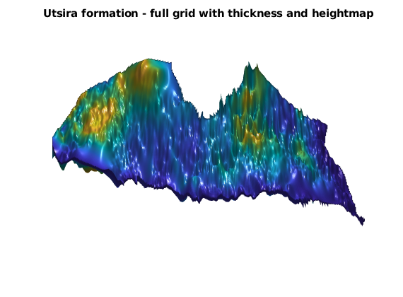
Full 3D visualization of all grids in North Sea¶

Not all formations in the data set supply both a height map of the top surface and a map of the formation thickness, which are both needed to construct a volumetric sandbody. Next, we visualize the different sandbodies that can be constructed based on pairs of depth and thickness maps. Because the grids are large, we will use functionality from the ‘opm_gridprocessing’ and ‘libgeometry’ mex-modules to speed up the processing.

% Load module
mrstModule add libgeometry opm_gridprocessing

% Count number of sand bodies
grdecls = getAtlasGrid(getNorthSeaNames(),'coarsening',10);
ng = numel(grdecls);

% Set view angles
viewMat = [-58 50; -90 65; -120 30; -120 30; -110 60; -110 60; ...
   -105 55; -105 -10; -95 40; -40 15; -90 80; -55 80; ...
   105 55; 60 20; -100 55; 90 45];

% Loop through and visualize all the 3D models at full resolution
for i=1:ng;
   grdecl = getAtlasGrid(grdecls{i}.name, 'coarsening', 1);
   try
      G = processgrid(grdecl{1});
      G = mcomputeGeometry(G(1));
   catch
      G = processGRDECL(grdecl{1});
      G = computeGeometry(G(1));
   end
   clf;
   plotGrid(G,'FaceColor', [1 .9 .9], 'EdgeAlpha', .05);
   view(viewMat(i,:)); axis tight off
   light('Position',[-1 -1 -1],'Style','infinite');lighting phong
   title(grdecls{i}.name)
   drawnow
end

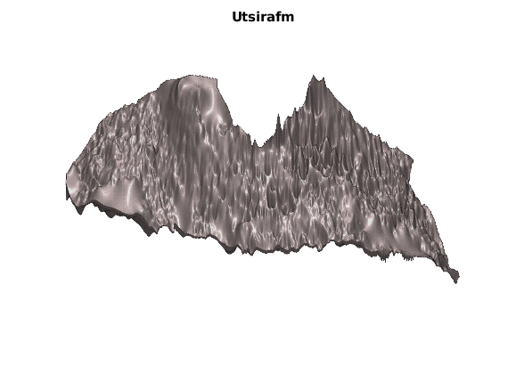
Basic capacity estimates for the CO2 atlas data (North Sea)¶

Finally, we compute the potential volumes available for structural trapping. To better report progress, we first load a low resolution version to get names of all aquifers. Then, we load and process the full-resolution versions to compute the geometrical volume inside all structural traps under each top surface

res = cell(ng,1);
fprintf('------------------------------------------------\n');
for i=1:ng
   fprintf('Processing %s ...
', grdecls{i}.name);
   grdecl  = getAtlasGrid(grdecls{i}.name, 'coarsening', 1);
   try
      G = mprocessGRDECL(grdecl{1});
      G = mcomputeGeometry(G(1));
   catch
      G = processGRDECL(grdecl{1});
      G = computeGeometry(G(1));
   end

   Gt = topSurfaceGrid(G);
   ta = trapAnalysis(Gt, false);

   res{i}.name      = grdecls{i}.name;
   res{i}.cells     = Gt.cells.num;
   res{i}.zmin      = min(Gt.cells.z);
   res{i}.zmax      = max(Gt.cells.z);
   res{i}.volume    = sum(G.cells.volumes);
   res{i}.trapvols  = volumesOfTraps(Gt,ta, []);
   res{i}.capacity  = sum(res{i}.trapvols);
   fprintf('done\n');
end

------------------------------------------------
Processing Brentgrp ... done
Processing Brynefm ... done
Processing Sleipnerfm ... done
Processing Fensfjordfm ... done
Processing Huginfmeast ... done
Processing Huginfmwest ... done
Processing Krossfjordfm ... done
...

Show table of volumes

fprintf('\n\nOverview of trapping capacity:\n')
fprintf('\n%-13s| Cells  | Min  | Max  | Volume   | Capacity  | Percent\n', 'Name');
fprintf('-------------|--------|------|------|----------|-----------|-----------\n');
for i=1:ng
   fprintf('%-13s| %6d | %4.0f | %4.0f | %4.2e |  %4.2e | %5.2f \n',...
      res{i}.name, res{i}.cells, res{i}.zmin, res{i}.zmax, res{i}.volume, ...
      res{i}.capacity, res{i}.capacity/res{i}.volume*100);
end
fprintf('-------------|--------|------|------|----------|-----------|-----------\n\n');

Overview of trapping capacity:

Name         | Cells  | Min  | Max  | Volume   | Capacity  | Percent
-------------|--------|------|------|----------|-----------|-----------
Brentgrp     |  21307 | 1659 | 5569 | 3.46e+12 |  9.63e+10 |  2.78
Brynefm      |  46754 |  271 | 4060 | 4.43e+12 |  3.37e+11 |  7.62
...

CO2 Storage Atlas: the Norwegian North Sea¶

Generated from showCO2atlas.m

The Norwegian Petroleum Directorate (NPD) has developed an atlas that gives an overview over areas in the Norwegian part of the North Sea where CO2 can be stored safely in the subsurface for a long time, see http://www.npd.no/en/Publications/Reports/CO2-Storage-Atlas-/. As part of the atlas, NPD has released geographical data for many of the formations that are described in the atlas. The data are given in a GIS formate (shape- and rasterfiles) and can be downloaded from their webpage. One of the purposes of the ‘co2lab’ in MRST is to provide simple access to public datasets. In this example, we describe how you can use the functionality in ‘co2lab’ to download and display the data sets that accompany the atlas. For the sake of convenience, we have converted the files to an ASCII format more suitable for our applications. These files can be inspected using any text editor. We also process the files and get both the raw datasets and data structures suitable for constructing volumetric corner-point grids of several sand bodies. At the end of the example, we analyse the different formations and compute the capacity for structural trapping in each formation.

Read data¶

This example assumes that you have already downloaded the North Sea datasets from the NPD webpages. If you have not done so, you can use the following command: downloadDataSets(‘atlas’)

mrstModule add co2lab deckformat

fprintf('Loading atlas data (this may take a few minutes)..');
[grdecls, rawdata] = getAtlasGrid(getNorthSeaNames()); %#ok
fprintf('done\n');

Loading atlas data (this may take a few minutes)..done

Description of raw data¶

Show the raw data. Each dataset contains four fields: - Name, which is the name of the formation - Variant: Either thickness or height, indicating wether the dataset represents height data or thickness data. - Data: The actual datasets as a matrix. - Meta: Metadata. The most interesting field here is the xllcorner/yllcorner variable which indicates the position in ED50 datum space.

fprintf('\nRaw data:\n')
fprintf('----------------------------------------------------------------\n');
for i=1:numel(rawdata);
    rd = rawdata{i};
    fprintf('Dataset %-2i is %-12s (%-9s). Resolution: %4i meters\n', ...
            i, rd.name, rd.variant,  rd.meta.cellsize)
end
fprintf('----------------------------------------------------------------\n');

% Store names for convenience
names = cellfun(@(x) x.name, rawdata, 'UniformOutput', false)';

Raw data:
----------------------------------------------------------------
Dataset 1  is Brentgrp     (thickness). Resolution:  500 meters
Dataset 2  is Brynefm      (thickness). Resolution:  500 meters
Dataset 3  is Cookfm       (thickness). Resolution:  500 meters
Dataset 4  is Dunlingp     (top      ). Resolution:  500 meters
Dataset 5  is Fensfjordfm  (thickness). Resolution:  500 meters
...

Show the data directly: Utsira formation¶

The datasets are perfectly usable for visualization on their own. To see this, we find the datasets corresponding to the Utsira formation and plot both the thickness and the heightmap. Note that the datasets are not entirely equal: Some sections are not included in the thickness map and vice versa. In addition to this, the coordinates are not always overlapping, making interpolation neccessary. Some formations are only provided as thickness maps; These are processed by sampling the relevant part of the Jurassic formation for top surface structure.

utsira_rd = rawdata(strcmpi(names, 'Utsirafm'));
clf;
for i = 1:numel(utsira_rd)
    urd = utsira_rd{i};

    subplot(2,1,i)
    surf(urd.data)

    title([urd.name ' ' urd.variant])
    shading interp
    view(0,90)
    axis tight off
end

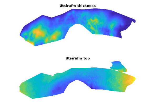
Visualize all the formations¶

We then visualize the formations present in the North Sea along with a map of Norway and point plots of all production wells in the Norwegian Continental Shelf. The well data comes from the Norwegian Petroleum Directorate and can be found in more detail at http://factpages.npd.no/factpages/. The map of Norway comes from The Norwegian Mapping and Cadastre Authority and can be found at http://www.kartverket.no/. Note that the map is only provided for scale and rough positioning - no claims are made regarding the accuracy in relation the subsea reservoirs. To visualize the formations, we load a 5x5 coarsened version of each data set and use this to create a simple volumetric model that represents approximately the outline of each formation. More details about how to create 3D grid models are given in the script ‘modelsFromAtlas.m’

grdecls = getAtlasGrid(getNorthSeaNames(),'coarsening', 5);
ng = numel(grdecls);

grids = cell(ng,1);
for i = 1:ng
    gd = processGRDECL(grdecls{i});
    grids{i} = computeGeometry(gd(1));
end
clf;
mymap = [
         0         0    1.0000
         0    1.0000         0
    1.0000         0         0
         0         0    0.5000
         0    0.5000         0
    0.7500         0         0
         0    1.0000    1.0000
    1.0000         0    1.0000
    1.0000    1.0000         0
    0.8500    0.8500    0.8500
    0.4000    0.4000    0.4000
         0         0         0
    0.2500    0.5000    1.0000
    0.5000    0.2500    0.7500
    0.7500    0.2500    0.5000
    0.7500    0.5000    0.2500
    0.2500    1.0000    0.5000
    0.5000    1.0000    0.2500
         ];
hold on

for i=1:ng;
    G = grids{i};
    bf = boundaryFaces(G);
    ind = G.faces.normals(bf,3)==0;
    plotFaces(G,bf(ind), 'FaceColor', 'none', 'EdgeColor', mymap(i,:), 'LineWidth',2);
%    % We want to colorize each grid differently
%    data = repmat(i, G.cells.num, 1);
%    plotCellData(grids{i}, data, 'facea', .3, 'edgea', .05, 'edgec', 'k');
end

legend(cellfun(@(x) x.name, grdecls, 'UniformOutput', false), ...
   'Location', 'EastOutside')
box on
view(2)
set(gcf,'Color',[0.8 0.8 0.8]);set(gca,'Color',[0.8 0.8 0.8]);
set(gca,'XColor',[0,0,0])
set(gca,'YColor',[0,0,0]);set(gca,'LineWidth',1)

ax = axis();
colormap hsv

% Load and plot a map
%load(fullfile(mrstPath('co2lab'), 'data', 'atlas', 'norway.mat'));
load(fullfile(getDatasetPath('co2atlas'), 'norway.mat'));
for k=1:length(norway),
    line(norway{k}(:,1) + 6.8e5, norway{k}(:,2));
end;
axis(ax)

hold on
%load(fullfile(mrstPath('co2lab'), 'data', 'atlas', 'welldata.mat'));
load(fullfile(getDatasetPath('co2atlas'), 'welldata.mat'));
plot(welldata(:,2), welldata(:,1), '.k', 'MarkerSize', 5)

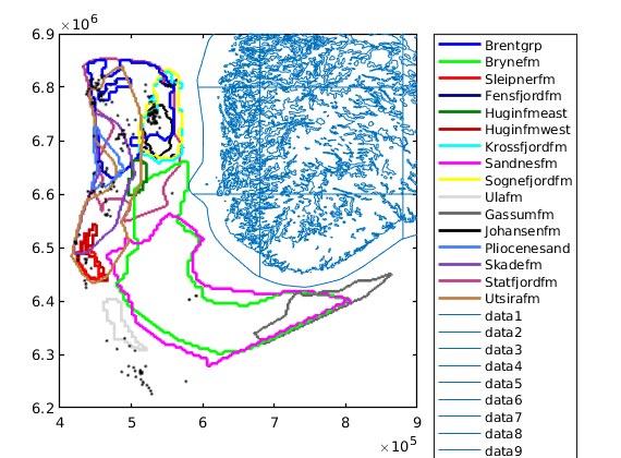
Redo the visualization in 3D with higher resolution¶

To show the depth of the various North Sea formations, we redo the plot in 3D.

figure;
p = get(gcf,'Position'); set(gcf,'Position', p + [-300 0 300 0]);
grdecls = getAtlasGrid(getNorthSeaNames(),'coarsening', 3);
ng = numel(grdecls);

grids = cell(ng,1);
for i = 1:ng
    gd = processGRDECL(grdecls{i});
    grids{i} = computeGeometry(gd(1));
end

clf;
hold on
for i=1:ng;
    G = grids{i};
    % We want to colorize each grid differently
    data = repmat(i, G.cells.num, 1);
    plotCellData(grids{i}, data, 'facea', .8, 'edgea', .01, 'edgec', 'k');
end
axis tight; box on; view(-300,50)
hold off
legend(cellfun(@(x) x.name, grdecls, 'UniformOutput', false), ...
   'Location', 'EastOutside')

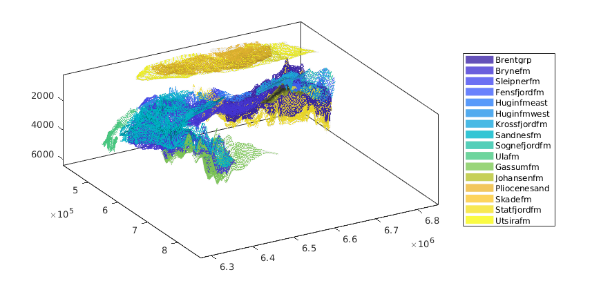
Johansen formation: the effect of coarsening on trapping¶

Generated from coarseningEffects.m

When working with subsea reservoirs coarsening will always be a factor:

This example demonstrates the effects of geometry coarsening on a model from the CO2 Storage Atlas grids, with a special focus on structural trapping. To this end, we generate six realizations of the Johansen formation: The first is the full dataset, the second coarsened by a factor 2 in both i and j directions, the third a factor 3, and so on. This gives a set of grids where the finest has approximately 80,000 cells, while the most coarse has ~2,000 cells. In the finest grid, each cell has a resolution of 500x500 m^2 per cell, while the coarsest has 3000x3000 m^2. The resolution in both grids is fairly large in compared with typical simulation grids in petroleum application.

mrstModule add co2lab coarsegrid deckformat

N = 6;
[Grids, res] = deal(cell(numel(N),1));
for i = 1:N
    fprintf(1,'\nLoading Johansen formation (coarsening factor: %d)...\n', i);
    gr = getAtlasGrid('Johansenfm', 'coarsening', i);
    G = processGRDECL(gr{1});
    % Create top surface grid
    Gt = topSurfaceGrid(computeGeometry(G(1)));
    Grids{i} = Gt;
    % Create trapping and store volumes of each trap
    res{i} = trapAnalysis(Gt, true);
    res{i}.volumes = volumesOfTraps(Gt, res{i}, []);
end

Loading Johansen formation (coarsening factor: 1)...
Loading module matlab_bgl
Trap level 1: 1301 traps identified
Trap level 2: 183 traps identified
Trap level 3: 25 traps identified
Trap level 4: 6 traps identified
Trap level 5: 2 traps identified
...

Plot a subset of the formation with different degree of coarsening¶

We first define a subdomain consisting of a minimum and maximum value for both x and y coordinates which is then plotted on the fine grid.

G = Grids{1};

subdomain = [5.25e5, 6.70e6; 5.30e5, 6.75e6];

x = G.cells.centroids(:,1);
y = G.cells.centroids(:,2);

subset = x > subdomain(1,1) & x < subdomain(2,1) &...
         y > subdomain(1,2) & y < subdomain(2,2);
clf;
plotCellData(G, G.cells.z,'EdgeColor','none')
plotGrid(G, subset, 'EdgeColor', 'None', 'FaceColor', 'black', 'FaceAlpha', .5)

axis tight off

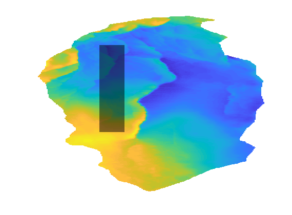
We can then loop over the grids while plotting the parts of the grid within the bounding box with a small height offset to visualize the fine scale details that are lost when coarsening the fine scale data. Note that there are several features in the topmost finest grid that have disappeared when coarsening: In the coarsest plot at the bottom almost all details are lost except for the rightmost fault.

clf
colors = {'b', 'r', 'g', 'c', 'm', 'y'};
colorize = @(i) colors{mod(i, length(colors)) + 1};
for i = 1:N

   G = Grids{i};
   G.nodes.z = G.nodes.z + 1000*i;

   x = G.cells.centroids(:,1);
   y = G.cells.centroids(:,2);
   subset = x > subdomain(1,1) & x < subdomain(2,1) &...
            y > subdomain(1,2) & y < subdomain(2,2);

   plotGrid(G, subset, 'facec', colorize(i), 'edgec', 'k', 'edgea', .3)
   fprintf('Grid with coarsening %d has %d fine cells and z-standard deviation %2.4f\n', ...
      i, G.cells.num, std(G.cells.z))
end
title('Coarsening of subset')
legend(regexp(num2str((1:N)*500), '  ', 'split'), 'Location', 'EastOutside')
view(86, 12)
axis tight off

Grid with coarsening 1 has 79422 fine cells and z-standard deviation 336.6869
Grid with coarsening 2 has 19454 fine cells and z-standard deviation 333.0837
Grid with coarsening 3 has 8476 fine cells and z-standard deviation 329.6796
Grid with coarsening 4 has 4674 fine cells and z-standard deviation 325.8592
Grid with coarsening 5 has 2936 fine cells and z-standard deviation 322.1026
Grid with coarsening 6 has 2000 fine cells and z-standard deviation 318.8460

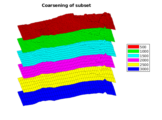
The effect of coarsening on trapping analysis¶

It is obvious that fine structural details are lost when coarsening the grids. The coarsening operation acts as a smoother on the grid, removing ridges, folds and oscillations that are present on a shorter wavelength than the coarse cells. Unfortunately, these small oscillations are especially interesting for CO2 migration studies: Small local height maxima can divert small “rivers” of CO2 and act as structural traps. To demonstrate that these traps are lost when coarsening, we plot the structural traps estimated by trapAnalysis for the different grids. Note that several smaller traps are removed as the coarsening increases, which can be shown statistically by noting that the mean of the trap volume quickly increases as the smaller traps are smoothed away. The total trapping volume also changes as the coarsening is increased: In the beginning the volume increases as the largest traps become slightly larger due to the lower resolution. Later on, the total volume shrinks as smaller traps are removed entirely.

% Plot the traps
clf
defaultpos = get(0, 'DefaultFigurePosition');
set(gcf, 'Position', [defaultpos(1:2) - [0 100], 1000 500]);
subplot('position', [.025 .025 .65 .925]);
for i = 1:N
    G = Grids{i};
    G.nodes.z = G.nodes.z + 1000*i;

    x = G.cells.centroids(:,1);
    y = G.cells.centroids(:,2);
    subset = x > subdomain(1,1) & x < subdomain(2,1) &...
             y > subdomain(1,2) & y < subdomain(2,2);

    plotGrid(G, subset, 'facec', colorize(i), 'facea', .2, ...
       'edgec', colorize(i), 'edgea', .9)

    tr = res{i};
    G_flat = flattenTraps(G, tr);
    G_flat.nodes.z = G_flat.nodes.z + 1000*i;
    plotGrid(G_flat, subset & tr.traps ~= 0, ...
       'FaceColor', colorize(i), 'EdgeColor', 'none')
end
% view(-30, 60)
view(86, 12)
axis tight off
title('Traps for successively coarsed grids')

% Plot the total volume as subplot
axes('position', [.75 .55 .225 .375]);
hold on
vol = cellfun(@(x) sum(x.volumes), res);
for i = 1:N
    bar(i, vol(i), colorize(i))
end
title('   Total trap volume')
set(gca, 'Color', get(gcf, 'Color'), ...
   'XTickLabel', regexp(num2str((1:N)*500), '  ', 'split'))
axis tight

% Plot the average volume as subplot
axes('Position', [0.75 .05 .225 .375])
hold on
mvol = cellfun(@(x) mean(x.volumes), res);
for i = 1:N
    bar(i, mvol(i), colorize(i))
end
title('     Average trap volume')
set(gca, 'Color', get(gcf, 'Color'), ...
   'XTickLabel', regexp(num2str((1:N)*500), '  ', 'split'))
axis tight

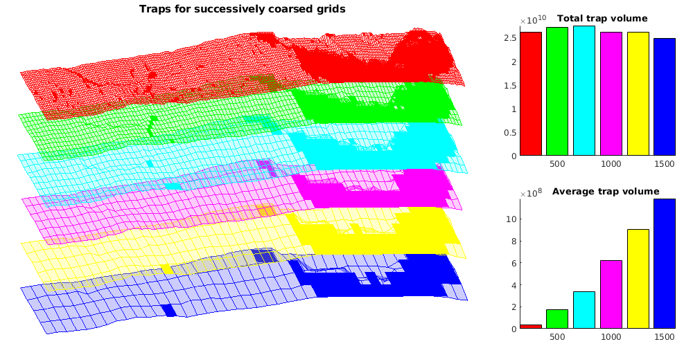
Trapping example¶

Generated from firstTrappingExample.m

In this example, we demonstrate the basic routines for computing traps, accumulation areas, spill paths, etc. To this end, we will use a simple shoe-box with a dip and a perturbed top surface.

mrstModule add co2lab coarsegrid

Make grid and rock data¶

We consider a sandbox of dimensions 10 km x 5 km x 50 m, that lies at a depth of 1000 m and has an inclination in the x-direction. For the top surface, we add a smooth sin/cos perturbation that will create domes. The porosity is set uniformly to 0.25

[Lx,Ly,H] = deal(10000, 5000, 50);
G  = cartGrid([100 100 1],[Lx Ly H]);
x  = G.nodes.coords(1:G.nodes.num/2,1)/Lx;
y  = G.nodes.coords(1:G.nodes.num/2,2)/Ly;
z  = G.nodes.coords(1:G.nodes.num/2,3)/H;
zt = z + x - 0.2*sin(5*pi*x).*sin(5*pi*y.^1.5) - 0.075*sin(1.25*pi*y) + 0.15*sin(x+y);
zb = 1 + x;
G.nodes.coords(:,3) = [zt; zb]*H+1000;
G = computeGeometry(G);

Construct top surface grid¶

We create a hybrid grid that represents the top surface. The grid is a 2D grid defined as a surface in 3D and contains a mapping from the 2D cells on the surfrace to the column of volumetric cells that lie below in the 3D grid. For visualization purposes, we create an extra grid that lies above the true top surface.

Gt = topSurfaceGrid(G);

figure;
Gt_zshifted = Gt;
Gt_zshifted.nodes.z = Gt_zshifted.nodes.z - 15;
plot_opts = {'edgeColor', 'k', 'edgeAlpha', 0.1};
plotGrid(G, plot_opts{:});
plotCellData(Gt_zshifted, Gt_zshifted.cells.z, plot_opts{:});
view(30,25); axis tight

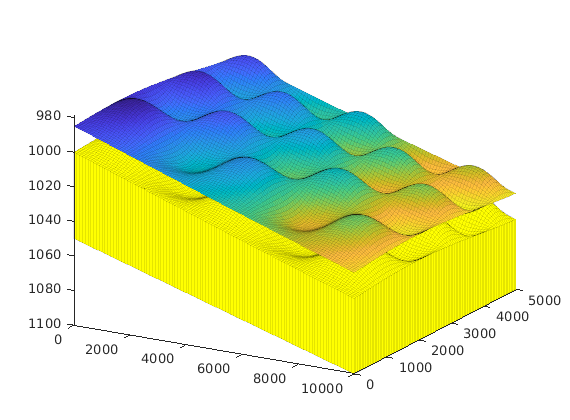
Geometric analysis of caprock (spill-point analysis)¶

Compute traps and spill paths connecting them. Here, we use the cell-based algorithm. The cells that belong to the identified traps are colored white in the plot

res = trapAnalysis(Gt, true);
num_traps = max(res.traps);
plotGrid(Gt_zshifted, res.traps>0, 'FaceColor','white', 'EdgeAlpha',.1);

Loading module matlab_bgl
Trap level 1: 13 traps identified
Start find rivers

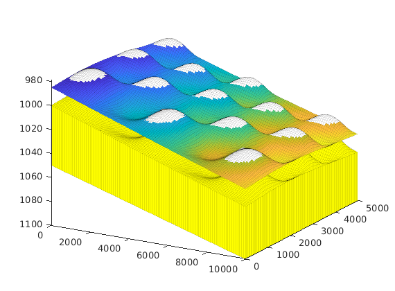
Show connection between traps and spill paths¶

We make a 2D plot of the top surface in which traps are colored red, cells that lie along the connecting spill paths are colored green, and the remaining cells are colored blue. In addition, we display the number associated with each trap slightly above its local maximum.

clf
fpos = get(gcf,'Position');
set(gcf,'Position',[300 400 800 420],'PaperPositionMode','auto');
trap_field = zeros(size(res.traps));
trap_field(res.traps>0) = 2;
for r = [res.cell_lines{:}]'
    for c = 1:numel(r)
        trap_field(r{c}) = 1;
    end
end

subplot(2,3,[1 4]);
plotCellData(Gt, trap_field, 'EdgeColor','none');
view(90,90); axis tight off

for i=1:num_traps
   ind = res.top(i);
   text(Gt.cells.centroids(ind,1),Gt.cells.centroids(ind,2), res.trap_z(i)-50,...
      num2str(res.traps(ind)), 'Color',.99*[1 1 1], ...
      'FontSize', 14, 'HorizontalAlignment','center');
end
colormap(jet);

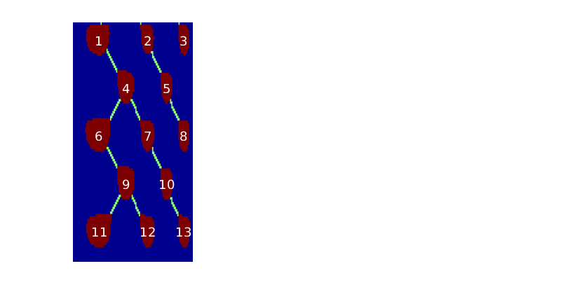
Compute the total trapping capacity¶

We compute the pore volume inside each of the traps, and report in descending order. In addition, we relate the trap volume to the total volume of the sandbox.

rock2D.poro = 0.25 * ones(G.cells.num, 1);
trap_volumes = volumesOfTraps(Gt, res, 1:num_traps, 'poro', rock2D.poro);

total_trapping_capacity = sum(trap_volumes);
pv = sum(poreVolume(Gt,rock2D));
fprintf('Total trapping capacity is: %6.3e\n', total_trapping_capacity);
fprintf('This amounts to %.2f %% of a total pore volume of %6.2e\n\n', ...
   total_trapping_capacity/pv*100, pv);
[sorted_vols, sorted_ix] = sort(trap_volumes, 'descend');

fprintf('trap ix   | trap vol(m3)  | cells in trap\n');
fprintf('----------+---------------+--------------\n');
tcells = zeros(num_traps,1);
for i = 1:num_traps
   tcells(i) = sum(res.traps == sorted_ix(i));
   fprintf('%7d   |  %10.3e   | %5d\n', ...
       sorted_ix(i), sorted_vols(i), tcells(i));
end
fprintf(['\nTogether, the five largest traps cover %6.2e m3, which represents %3.1f%% of' ...
   '\nthe total trapping capacity of this grid.\n'], ...
   sum(sorted_vols(1:5)), sum(sorted_vols(1:5)) / total_trapping_capacity * 100)

subplot(2,3,[2 3]);
bar(1:num_traps,sorted_vols);
set(gca,'XTickLabel',sorted_ix);
title('Trap volume (m^3)');

subplot(2,3,[5 6]);
bar(1:num_traps,tcells);
set(gca,'XTickLabel',sorted_ix);
title('Number of cells in trap');

Total trapping capacity is: 4.948e+06
This amounts to 39.58 % of a total pore volume of 1.25e+07

trap ix   | trap vol(m3)  | cells in trap
----------+---------------+--------------
      6   |   6.611e+05   |   245
     11   |   6.415e+05   |   241
      1   |   5.312e+05   |   210
...

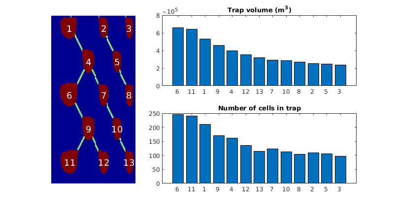
Plot leaf nodes¶

Next, we will look at leaf nodes in our trapping system, i.e., traps that only have outgoing ‘rivers’. The leaf traps are shown in white color. The drainage areas and the resulting migration path are given a unique color so that one can trace the migration of CO2 upward until it either leaves the formation or reaches a higher trap that accumulates CO2 from multiple leaf traps. All traps that are not leaf traps are shown in dark gray. To do this, we will utilize two functions that are called as part of trapAnalysis, but whose retun argument are not fully exposed by the higher-level interface in trapAnalysis.

moduleCheck('matlab_bgl');
ts         = findTrappingStructure(Gt);
trap_con   = findTrapConnections(Gt, ts.z_spill_loc);
traps      = trap_con.traps;
leaf_lines = trap_con.leaf_lines;
leaf_traps = trap_con.leaf_traps;

% Plot traps and grid
clf, set(gcf,'Position',fpos);
plotGrid(ts.Gtop, ts.z_spill_loc>0, 'EdgeColor', 'none', 'FaceColor',[.25 .25 .25])
plotGrid(ts.Gtop, 'FaceColor', 'none', 'EdgeAlpha', .1)

% Find leaves and the corresponding traps
[ll, tc, dc] = deal([]);
C    = maxTPFAGravityMatrix(ts.Gtop);
nll  = numel(leaf_lines);
p    = randperm(nll);
lvol = zeros(nll,1);
tic
for k=nll:-1:1
   % extract the leaf line out of the trap
   ll  = [ll; leaf_lines{k}', p(k)*ones(length(leaf_lines{k}),1)]; %#ok

   % find all cells in the given trap
   t_cells = find(traps ==leaf_traps{k});
   tc = [tc; t_cells]; %#ok

   % find all cells in the drainage region of the leaf
   cc = find( dfs(C', double(t_cells(1))) >0);
   dc  = [dc; cc, p(k)*ones(length(cc),1)]; %#ok

   % calculate the leaf volume
   cc = find( dfs(C, double(t_cells(1)))>0 );
   lvol(k) = sum((ts.Gtop.cells.z(cc) - Gt.cells.z(cc)).*Gt.cells.volumes(cc));
   disp(['Leaf volume : ', num2str(lvol(k))]);
end

% Plot leaves and the deepest traps
plotCellData(ts.Gtop, [ll(:,2); dc(:,2)], [ll(:,1); dc(:,1)], 'EdgeColor', 'none');
plotGrid(ts.Gtop, tc, 'EdgeColor', 'none', 'FaceColor', [.9 .9 .9]);
set(gca,'Projection','perspective');
view(120,25); axis tight

Loading module matlab_bgl
Trap level 1: 13 traps identified
Start find rivers
Leaf volume : 4088362.1192
Leaf volume : 5213223.2029
Leaf volume : 10751963.0795
Leaf volume : 9597653.0105
Leaf volume : 7304958.3348

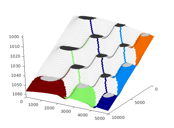
Plot accumulation areas using interactive viewer¶

Finally, we launch the interactive viewer. Here, each trap and the surrounding accumulation areas are given a unique color. Injection scenarios for a single well can be investigated by clicking on the surface (inside a trap or an accumulation region). This will compute the resulting spill-point path and the potential trapping volumes inside traps that are visited before the spill path exits the model.

h = interactiveTrapping(Gt, 'method', 'cell', 'light', true, ...
   'spillregions', true, 'colorpath', false, 'injpt', 1898);
view(80,20);
set(gca,'DataAspect', [2 1.5 .02]);

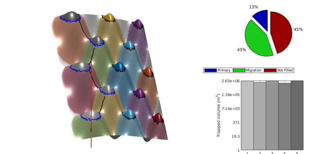
Optimal injection points¶

Generated from optimizationExample.m

In this example we demonstrate how information about structural traps and their connections can be used to define a good guess of injector placements. That is, we will consider the problem of determining where N wells should be placed to optimize the potential for structural trapping.

mrstModule add co2lab;

Extract a subset of the Utsira formation for analysis¶

coarsefactor = 2;
[grdecl, d, petrodata] = getAtlasGrid('utsirafm', 'coarsening', coarsefactor);
pd = petrodata{1};

G = processGRDECL(grdecl{1});
G = computeGeometry(G(1));
cdims = G.cartDims;
% G = extractSubgrid(G, find(G.cells.centroids(:, 2) > 6.62e6));
% G.cartDims = cdims;
% G = computeGeometry(G);

Gt = topSurfaceGrid(G);
rock = struct('poro', repmat(pd.avgporo, G.cells.num, 1), ...
              'perm', repmat(pd.avgperm, G.cells.num, 1));

Compute trapping analysis and find the sorted injection trees¶

An injection tree corresponds to a root node and all traps that are upstream from that node. By default, maximize trapping finds all leafnodes while accounting for overlap between the trees. We find both the trap tree with and without overlap. Once plotted, it is obvious that the calculated volumes with overlap are quite different from those without: As several leaf nodes may be downstream from the larger traps in any given tree, many trees will largely consist of the same traps. When optimizing injection with a single injection point the distinction is not important, but the overlap must be considered when

res = trapAnalysis(Gt, true);
trees = maximizeTrapping(Gt, 'res', res, 'removeOverlap', true);
trees_nooverlap = maximizeTrapping(Gt, 'res', res, 'removeOverlap', false);

Loading module matlab_bgl
Loading module coarsegrid
Trap level 1: 198 traps identified
Trap level 2: 29 traps identified
Trap level 3: 2 traps identified
Start find rivers

several injectors are being considered.

close all
fp = get(0, 'DefaultFigurePosition');
h = figure('position', fp.*[1 1 1 .5]);

[tv, tv_noop] = deal(nan(max(res.traps), 1));

% Index into total trap index based on leaf node
tv(vertcat(trees.root)) = vertcat(trees.value);
tv_noop(vertcat(trees_nooverlap.root)) = vertcat(trees_nooverlap.value);

% Sort by the overlapping values
[tv, ind] = sort(tv, 'descend');
tv_noop = tv_noop(ind);

% Strip nan values
tv_noop(isnan(tv)) = [];
tv(isnan(tv)) = [];

bar([tv, tv_noop- tv], 'stacked')
set(gcf, 'Renderer', 'painters')
ylabel('Tree volume (m^3)')
xlabel('Tree index')
caxis( [.5 2])
set(gca, 'Yscale', 'log')
axis auto
ylim([min(tv), 1.1*max(tv)])
legend({'Without overlap', 'Overlap'},'location', 'southwest')

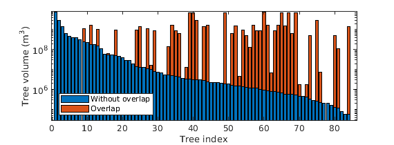
Find the ideal injection spot for each trap region¶

Use the largest z value to find the ideal injection spot: This corresponds to the deepest possible place in the reservoir surface to inject. We show the ten best root notes, which maximizes stored CO2 where five injectors are to be placed. We also find the best single injection cell if we assume that the boundary between two different trap regions spills over to both the neighboring trap regions.

mrstModule add mrst-gui;
if ishandle(h); close(h); end;
h = figure('position', fp.*[1 1 2.5 1.5]);

N = 10;
% Work out the lowest point in each root trap
trapcells = zeros(N, 1);
for i = 1:N
    r = res.trap_regions == trees(i).root;
    region = find(r);
    tmp = Gt.cells.z;
    tmp(~r) = -inf;

    [minpoint, cell] = max(tmp);
    trapcells(i) = cell;
end
% Get the best cell on a ridge
[bestSingleCell, largestVol, allFaces, point, traps] = findOptimalInjectionPoint(Gt, res);

% Vast differences in values, use log10
largest = log10(largestVol);
v       = log10(tv);
treestart = [largest; v(1:N)];
trapcells = [bestSingleCell; trapcells];

clf;
% Plot all traps colorized by their largest tree volume
plotted = false(G.cells.num, 1);
for i = 1:numel(trees)
    cells = ismember(res.traps, trees(i).traps);
    plotCellData(G, repmat(v(i), G.cells.num, 1), cells & ~plotted, ...
                 'EdgeColor','none');
    plotted = plotted | cells;
end

plotGrid(G, res.traps == 0, 'edgec', 'none', 'facec', [1 1 1]*.9)

plotBar = @(data, cells, format) plotGridBarchart(G, data, cells, ...
                            'widthscale', 5*(1/coarsefactor), 'facecolor', [], ...
                            'fontsize', 15, ...
                            'EdgeColor', 'none', 'textformat', format);
% Setup function handle to show percent of total trapped volume
perc = @(x) 100*(10^x)/sum(tv);
plotBar(treestart, trapcells, @(x) sprintf('%1.1f%%', perc(x)))

outlineCoarseGrid(G, res.trap_regions, 'facecolor', 'none')
% set(gca,'ZDir','normal');
camlight head
lighting phong
% set(gca,'ZDir','reverse');

axis tight off
view(64, 72)
caxis([min(treestart), max(treestart)]);

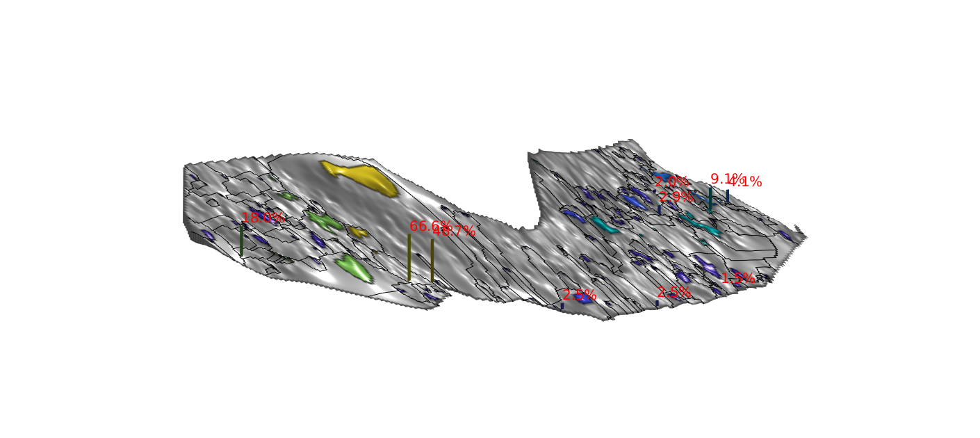
Alternative visualization¶

This is more dull, but has a somewhat higher information content

n = max(res.trap_regions);
c = jet(n); c=c(randperm(n),:);

subplot(1,2,2);
plotted = false(G.cells.num, 1);
for i = 1:numel(trees)
    cells = ismember(res.traps, trees(i).traps);
    plotCellData(G, repmat(v(i), G.cells.num, 1), cells & ~plotted, ...
                 'EdgeColor','none');
    plotted = plotted | cells;
end
colormap(jet(128));
contourAtlas(d{2},50,.25,.4*ones(1,3));
coord = Gt.cells.centroids(trapcells,:);
plot(coord(:,1),coord(:,2),'o',...
   'MarkerEdgeColor','b','MarkerFaceColor','r','LineWidth',3,'MarkerSize',8);

perc = @(x) 100*(10^x)/sum(tv);
plotBar(treestart, trapcells, @(x) sprintf('%1.1f%%', perc(x)))


subplot(1,2,1);
for i=1:n
   plotFaces(G,boundaryFaces(G,res.trap_regions==i), ...
      'EdgeColor','none','FaceColor', .5*c(i,:)+.5*ones(1,3));
end
plotFaces(G,boundaryFaces(G,res.trap_regions==0), ...
   'EdgeColor','none','FaceColor', .85*ones(1,3));
plotted = false(G.cells.num, 1);
for i = 1:numel(trees)
    cells = ismember(res.traps, trees(i).traps);
    plotCellData(G, repmat(v(i), G.cells.num, 1), cells & ~plotted, ...
                 'EdgeColor', 'none');
    plotted = plotted | cells;
end
colormap(jet(128));

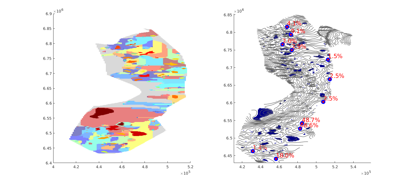
Top-Surface Grids¶

Generated from showTopSurfaceGrids.m

In this tutorial, we will go through the basics of the top-surface grids, showing how to construct them, and discussing some of the data structure.

mrstModule add co2lab

A simple 3D example: removing unconnected cells¶

We make a simple 3x3x3 Cartesian model with two cut-outs, one vertical and one horizontal. The grid is specified in a left-hand system so that the z-coordinate gives the depth, i.e., is increasing downwards.

clear, clc;
G = tensorGrid(0:3, 0:3, 2:0.5:3.5);
C = false([3 3 3]); C(3,1:2,2)=true; C(1,1,:) = true;
figure
subplot(1,2,1)
  plotCellData(G,reshape(double(C), [],1),'EdgeColor','k');
  view([20 20]), axis tight

G.nodes.coords(:,3) = G.nodes.coords(:,3) + ...
   0.125*sin(G.nodes.coords(:,1).*G.nodes.coords(:,2));
G = removeCells(G, find(C));
G = computeGeometry(G);
subplot(1,2,2)
  plotGrid(G); view([20 20]), axis tight

Construct top-surface grid¶

Column (1,1,:) is empty and hence the corresponding cell in the 2D top-surface grid is set as inactive. The horizontal cut-out in cells (3,1:2,2), on the other hand, induces lack of vertical connection in two of the grid columns and only the top part of the columns is used in the top-surface grid.

[Gtop,Gn] = topSurfaceGrid(G);
clf,
plotGrid(Gn,'FaceAlpha',1);
z = Gtop.nodes.z; Gtop.nodes.z = z - 0.15;
plotGrid(Gtop,'FaceColor','b');
Gtop.nodes.z = z;
view([30 30]), axis tight

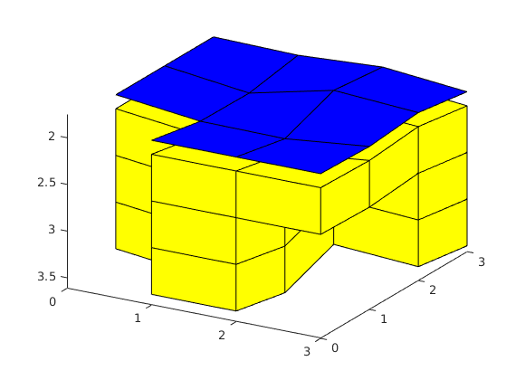
Inspect the data structure: planar 2D grid¶

The top-surface grid is represented as a standard 2D grid, which in MRST is assumed to be planar. The elevation of the surface is given by the field NODES.Z in the grid structure. Although this field is not part of the standard grid structure, plotGrid will check if it is present and then interpret the 2D grid as a (non-planar) 3D surface. Hence, we need to temporarily remove the field before plotting if we want only the planar 2D grid.

clf,
plotGrid(Gn);
z = Gtop.nodes.z;
Gtop.nodes = rmfield(Gtop.nodes,'z');
plotGrid(Gtop,'FaceColor','none','EdgeColor','r');
Gtop.nodes.z = z;
%
hold on;
plot3(Gtop.nodes.coords(:,1), Gtop.nodes.coords(:,2), z,'bo','LineWidth',2);
hold off;
view([30 30]); axis tight

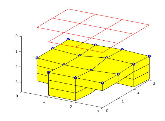
Numbering of cells in top-surface and 3D grid¶

The cells in the top-surface grid can be accessed using their cell number or through their logical ij-index given in the array CELLS.IJ. To find the centroids of the cells on the surface grid, we extend the centroids from the planar grid with the array CELLS.Z.

clf,
plotFaces(Gn,(1:Gn.faces.num)','FaceAlpha',0.5);
%plotGrid(Gtop,'FaceColor','r');
c  = [Gtop.cells.centroids Gtop.cells.z];
index = [(1:Gtop.cells.num)' Gtop.cells.ij];
text(c(:,1)-0.2,c(:,2)+0.2,c(:,3)-0.05, ...
   reshape(sprintf('%d: (%d,%d)', index'),8,[])');
view([-40 70]), axis tight off

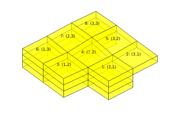
Likewise, there is a numbering of all nodes and faces. As above, we use the extra fields NODES.Z and FACES.Z to place the nodes and the centroids of the edges on the 3D top surface.

clf
plotGrid(Gtop,'FaceColor',[.9 .9 .9]);
hold on
c = [Gtop.nodes.coords Gtop.nodes.z];
plot3(c(:,1),c(:,2),c(:,3),'xr','MarkerSize',10);
text(c(:,1),c(:,2),c(:,3)-0.02,num2str((1:Gtop.nodes.num)'),...
   'Color','r','FontSize',12);
c = [Gtop.faces.centroids Gtop.faces.z];
plot3(c(:,1),c(:,2),c(:,3),'ob','MarkerSize',6);
text(c(:,1),c(:,2),c(:,3)-0.02,num2str((1:Gtop.faces.num)'),...
   'Color','b','FontSize',12);
hold off,
set(gca,'zlim',[1.8 2.2]), view([-15 65])

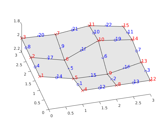
Each cell in the top-surface grid has a stack of cells attached to it. These stacks are defined by the array COLUMNS.CELLS, which maps to the indices of the cells in the corresponding 3D grid, and CELLS.COLUMNPOS, which is an indirection map into the COLUMNS.CELLS array.

clf
plotFaces(Gn,1:Gn.faces.num,'FaceAlpha',0.05);
hold on;
c = Gn.cells.centroids;
plot3(c(:,1),c(:,2),c(:,3),'or');
i = Gtop.columns.cells;
text(c(i,1),c(i,2),c(i,3),num2str(i));
hold off
view([25 75]), axis tight off

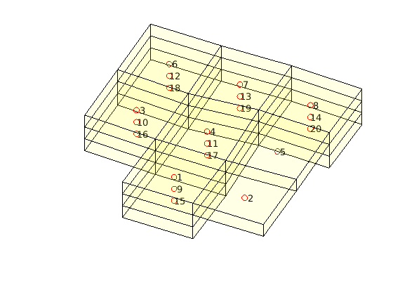
Geometry information¶

The array COLUMNS.Z gives the height of the centroid of the bottom surface of each 3D cell defined relative to the top surface (shown in light red). The array CELLS.H gives the total height of the cell column, i.e., the height difference between the top surface (in light red) and the bottom surface (in light blue).

clf
c = Gtop.cells.centroids;
i = rldecode(1:Gtop.cells.num, diff(Gtop.cells.columnPos),2)';
hold on
plot(c(:,1),c(:,2), 'ro');
plot3(c(i,1),c(i,2),Gtop.columns.z,'b*');
plot3(c(:,1),c(:,2),Gtop.cells.H, 'gs');
hold off
legend('cells.centroids','columns.z','cells.H','Location','EastOutside')

z = Gtop.nodes.z;
Gtop.nodes = rmfield(Gtop.nodes,'z');
plotGrid(Gtop,'FaceColor','r','EdgeColor','r','FaceAlpha',0.05);
Gtop.nodes.z = z;

% Hardcoded way of finding cell nodes - only works for quadrilateral cells
faceNodes = reshape(Gtop.faces.nodes,2,[])';
nodes = reshape(faceNodes(Gtop.cells.faces,:)',[],1);
cn = reshape(nodes,8,[]);
cn = cn(:,1:Gtop.cells.num);
cn = cn([1 3 6 8],:);
X = reshape(Gtop.nodes.coords(cn,1),4,[]);
Y = reshape(Gtop.nodes.coords(cn,2),4,[]);
H = repmat(Gtop.cells.H,[1 4])';
patch(X,Y,H,'b','FaceColor','b','EdgeColor','b','FaceAlpha',0.05);

view([-65 30]), axis tight

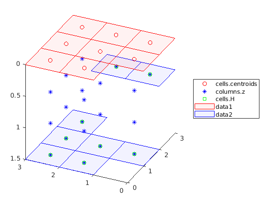
Miscellaneous¶

The top-surface grid consists of a subset of the faces in the 3D grid. These subfaces can be accessed using the array CELLS.MAP3DFACE. For convenience, the corresponding surface normals are stored in the array CELLS.NORMALS

clf,
plotGrid(Gn,'FaceAlpha',0.5);
plotFaces(Gn,Gtop.cells.map3DFace(1:Gtop.cells.num),'FaceColor','r')
view([30 50]), axis tight
c = [Gtop.cells.centroids Gtop.cells.z];
n = -Gtop.cells.normals;
hold on
quiver3(c(:,1),c(:,2),c(:,3),n(:,1),n(:,2),n(:,3),.5);
hold off;

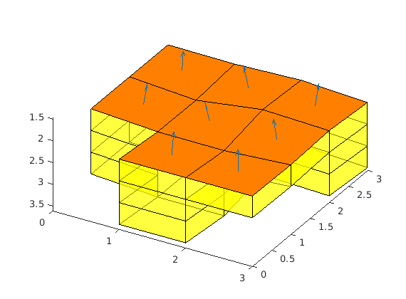
Interactive spill point analysis of top surface grids¶

Generated from showTrapsInteractively.m

This example demonstrates the use of the interactive viewer for viewing and finding structural traps for CO2 migration. Three different examples are presented:

The following functionality is present in the interactive viewer: - Left clicking on a trap will colorize the trap and all other traps that are downstream to that trap along with the path between them. Left clicking shows an estimate of where and how any slowly injected CO2 will migrate from the click position. When left-clicking, two additional plots are produced:

Right or ctrl-clicking on a trap will open a new plot showing the trap in detail along with the region around it. The largest possible structural trapping volume for the region will be indicated in red and blue.
Middle mouse or shift-clicking on a trap will show all traps that are upstream to the current trap much in the same manner as left mouse click. This can be used to find possible injection sites which will migrate over time to a large reservoir volume.
The toolbar in the figure window has several functions:

mrstModule add co2lab coarsegrid
% Select trapping algorithm
useCell = true;

switch useCell
    case true
        method = 'cell';
    otherwise
        method = 'node';
end

% Check if the script is run interactively, or as a standalone script
isScript = numel(dbstack) == 1;

Explore a synthetic grid¶

We first create a simple synthetic grid to demonstrate the interactive trapping. This grid is created by producing a simple Cartesian geometry and perturbing the z coordinates by a periodic function based on x and y to get several local traps. Additionally, to create a hierachy of traps, we slant the grid. We plot the top surface grid in the interactive viewer. Initially the possible structural traps are shown, colorized by the volume of each structural trap on a white grid.

L = 1000; L_p = L/5; H = 10;
G = cartGrid([101 101 1],[L L H]);
G.nodes.coords(:,3) =   100 + G.nodes.coords(:,3) + ...
                              G.nodes.coords(:,1)*0.01...
                    -2*sin(pi*G.nodes.coords(:,1)/L_p).*...
                       sin(pi*G.nodes.coords(:,2)/L_p);
G = computeGeometry(G);

% Create top surface grid
Gt = topSurfaceGrid(G);

% Show interactive plot
h = interactiveTrapping(Gt, 'method', method, 'light', true);
view(180, 50)

disp('Showing synthetic dataset...
Close to continue')
if isScript
    waitfor(h)
end

Current positition is not downstream from any trap, or spillpoint data was not produced.
Showing synthetic dataset... Close to continue

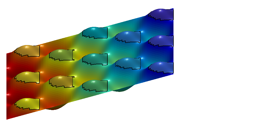
The Johansen formation¶

By passing in the name of a CO2 Storage Atlas grid, the function automatically generates the grid for us. We select the Johansen formation and apply some coarsening to make the grid smaller. Note that full resolution should be used if possible to get the best accuracy.

h = interactiveTrapping('Johansenfm', 'coarsening', 2, ...
   'method', method, 'light', true, 'contour', true);
view(-70, 80)

disp('Showing CO2 Atlas dataset...
Close to continue')
if isScript
    waitfor(h)
end

Current positition is not downstream from any trap, or spillpoint data was not produced.
Showing CO2 Atlas dataset... Close to continue

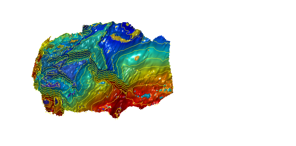
Grid from the IGEMS¶

The purpose of the IGEMS project was to study the impact that top-surface morphology has on storage capacity and the migration process. Alternative top-surface morphologies are created stochastically by combining different stratigraphic scenarios with different structural scenarios. For more information about the data set, see http://files.nr.no/igems/data.pdf.

G = readIGEMSIRAP('OSS', 1, 'coarse', [2 2]);
Gt = topSurfaceGrid(G);

% Activate trapping
h = interactiveTrapping(Gt, 'method', method);
view(180, 50)

disp('Showing IGEMS dataset...
Close to continue')
if isScript
    waitfor(h)
end

Current positition is not downstream from any trap, or spillpoint data was not produced.
Showing IGEMS dataset... Close to continue

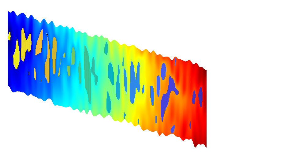
Effects of scales structures on trapping capacity¶

Generated from subscaleResolution.m

The CO2 Storage Atlas grids are very coarse, even at the finest resolution supplied. As they cover vast scales and were meant for mapping, this is to be expected. To give an indication of the subscale morphology and potential traps that are not resolved in the atlas models, we will use a data model of Sleipner, which is the world’s first subsea CO2 storage site and is located in the larger Utsira formation. The model was originally developed by Statoil has much higher spatial resolution. The model was publicly released by IEA and could be downloaded from their webpage by registred users: http://www.ieaghg.org/index.php?/20110329248/sleipner-benchmark-model.html

Altogether, the example shows the importance of using fine-scale resolution when simulating long-term migration because coarsening may have a large impact on the trapped CO2 volumes.

mrstModule add co2lab

Load data and create grids¶

fprintf('Constructing Sleipner model...');
datapath = getDatasetPath('sleipner');
sleipner_deck = readGRDECL(fullfile(datapath, 'M9X1.grdecl'));

% Do mapaxis explicitly to get coinciding coordinate systems
ma = [436914 6475050 436914 6469150 440114 6469150];
coord = reshape(sleipner_deck.COORD,3,[])';
coord(:,1:2) = mapAxes(coord(:,1:2), ma);
coord = coord';
sleipner_deck.COORD=coord(:);

% Create top-surface grids for Sleipner
G_sleipner  = processGRDECL(sleipner_deck);
G_sleipner  = computeGeometry(G_sleipner);
Gt_sleipner = topSurfaceGrid(G_sleipner);
fprintf('done\n');

% Create top-surface grids for Utsira (uncoarsened)
fprintf('Constructing Utsira model...');
grdecl_utsira = getAtlasGrid('Utsirafm', 'coarsening', 1);
G_utsira = processGRDECL(grdecl_utsira{1});
Gt_utsira = topSurfaceGrid(G_utsira);
fprintf('done\n');

Constructing Sleipner model...done
Constructing Utsira model...done

Trap analysis¶

res_sleipner = trapAnalysis(Gt_sleipner, true);
res_utsira = trapAnalysis(Gt_utsira, true);

Loading module matlab_bgl
Loading module coarsegrid
Trap level 1: 196 traps identified
Trap level 2: 34 traps identified
Trap level 3: 2 traps identified
Trap level 4: 1 traps identified
Warning: purging 4 bad traps with 0 spill value.
Start find rivers
...

We create a bounding box approximately equal to the fine Sleipner grid and use it to plot the corresponding area of the Utsira formation. The Sleipner grid is shown along with all local traps. As can be seen from the figure, what is a smooth surface in the coarse Utsira grid has several fine scale structures in the Sleipner grid, leading to several traps and potential rivers.

xs = Gt_sleipner.nodes.coords(:,1);
ys = Gt_sleipner.nodes.coords(:,2);

x = Gt_utsira.cells.centroids(:,1);
y = Gt_utsira.cells.centroids(:,2);
region = min(xs) < x & x < max(xs) & min(ys) < y & y < max(ys);

% Plot the grid
clf;
plotGrid(Gt_utsira, region, 'facec', [1 .6 .6])
plotGrid(Gt_sleipner, res_sleipner.traps == 0, 'facec', 'none', 'edgea',.2)
plotCellData(Gt_sleipner, res_sleipner.traps, res_sleipner.traps ~= 0, 'edgec', 'none')
view(-40, 50)
axis tight off
title('Utsira subset and Sleipner grid')

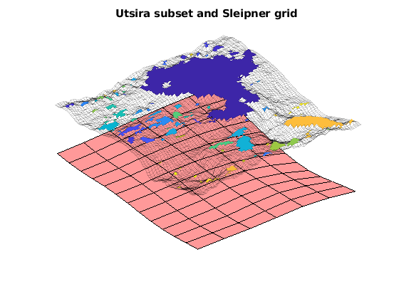
Estimate the unresolved local oscillations per area¶

We find the total trap volume for Sleipner and divide it by the total area of the Sleipner case to find a rough estimate of the trap volume per area from small-scale oscillations. Note that we are always using volume in the geometrical sense: To find the amount of CO2 stored, both a porosity and a reference density of CO2 is required.

trapvol_sleipner = sum(volumesOfTraps(Gt_sleipner, res_sleipner, []));
area_sleipner = sum(Gt_sleipner.cells.volumes);

finescaletraps = trapvol_sleipner/area_sleipner;
fprintf(['\nBy using the Atlas grid, approximately %2.5g liters of trapping\n'...
         'volume is not resolved per m^2 of area\n'], 1000*finescaletraps);

By using the Atlas grid, approximately 559.93 liters of trapping
volume is not resolved per m^2 of area

Extrapolate this estimate to the whole Utsira formation¶

trapvol_utsira = sum(volumesOfTraps(Gt_utsira, res_utsira, []));

area_utsira = sum(Gt_utsira.cells.volumes);
lost_volume = area_utsira*finescaletraps;
fprintf(['Total approximate unresolved trap volume for Utsira: %2.5g liters\n'...
        '(%1.2f%% of estimated large-scale trapped volume)\n'],...
        1000*lost_volume, 100*lost_volume./trapvol_utsira);

Total approximate unresolved trap volume for Utsira: 1.3768e+13 liters
(81.76% of estimated large-scale trapped volume)

Get another estimate by removing global trends¶

This estimate is obviously quite large as there may be global traps included in the fine Utsira grid that are counted twice. As we are primarily interested in structural traps that are smaller than what can be resolved by the coarse grid, we can obtain a more conservative estimate by removing the overall trends in the Utsira grid from the Sleipner grid and recomputing the traps. This is done by creating an interpolant from the Utsira top-surface grid and sampling the interpolant in the corresponding fine coordinates to obtain new z values. The three grids are plotted: Note how the adjusted grid (in green) has less curvature as it intersects the original grid, while having less traps volume. The largest trap is significantly reduced once the trend has been removed.

zinterp = TriScatteredInterp(Gt_utsira.cells.centroids(:, 1), ...
                             Gt_utsira.cells.centroids(:, 2), ...
                             Gt_utsira.cells.z(:));

Gt_adjusted = Gt_sleipner;

% Adjust z values by subtracting the interpolated z value and adding the
% average value in the area.
adjust = @(z, xy) z - zinterp(xy(:,1), xy(:,2)) + mean(Gt_utsira.cells.z(region));

Gt_adjusted.cells.z = adjust(Gt_adjusted.cells.z, Gt_adjusted.cells.centroids);
Gt_adjusted.faces.z = adjust(Gt_adjusted.faces.z, Gt_adjusted.faces.centroids);
Gt_adjusted.nodes.z = adjust(Gt_adjusted.nodes.z, Gt_adjusted.nodes.coords);

% Recompute geometry to get correct centroids
Gt_adjusted = computeGeometryVE_2D(Gt_adjusted);

res_adjusted = trapAnalysis(Gt_adjusted, true);

clf;
% Plot adjusted grid with traps
plotGrid(Gt_adjusted, res_adjusted.traps == 0, 'facea', .5, 'facec', 'green')
plotCellData(Gt_adjusted, res_adjusted.traps, res_adjusted.traps ~= 0, 'edgec','none')

% Plot original grid with traps
plotCellData(Gt_sleipner, res_sleipner.traps, res_sleipner.traps~=0, 'edgec','none')
plotGrid(Gt_sleipner, res_sleipner.traps == 0, 'facea', .3, 'facec', 'blue')

% Plot the Utsira grid showing the general trend being removed
plotGrid(Gt_utsira, region, 'facec', 'red')

view(-50, 40);
axis tight off

title('Adjusted versus original Sleipner grid')

Loading module matlab_bgl
Loading module coarsegrid
Trap level 1: 179 traps identified
Trap level 2: 22 traps identified
Trap level 3: 2 traps identified
Warning: purging 4 bad traps with 0 spill value.
Start find rivers

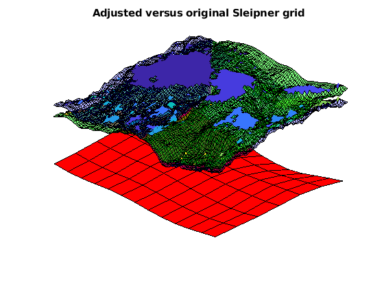
Find new trapping volume¶

trapvol_adjusted = sum(volumesOfTraps(Gt_adjusted, res_adjusted, []));

finescaletraps = trapvol_adjusted/area_sleipner;
fprintf(['\nBy using the Atlas grid, approximately %2.5g liters of trapping\n'...
         'volume is unresolved per m^2 of area\n'], 1000*finescaletraps);

By using the Atlas grid, approximately 210.29 liters of trapping
volume is unresolved per m^2 of area

Extrapolate this estimate to the whole Utsira formation¶

lost_volume_adjusted = area_utsira*finescaletraps;
fprintf(['Total approximate unresolved trap volume for Utsira ' ...
        '(with global trends removed):\n'...
        '%2.5g liters (%1.2f%% of estimated large scale trapped volume)\n'],...
         1000*lost_volume_adjusted, 100*lost_volume_adjusted./trapvol_utsira);

Total approximate unresolved trap volume for Utsira (with global trends removed):
5.1708e+12 liters (30.71% of estimated large scale trapped volume)

Compare trap of local variations to global variations¶

Shown as a pie chart, it is obvious that fine-scale variations in tje top-surface geometry contribute a significant volume to structural trapping compared to the large-scale structural traps. This shows the importance of using fine-scale resolution when simulating long-term migration because coarsening may have a large impact on the trapped CO2 volumes.

figure
pie([lost_volume_adjusted trapvol_utsira])
legend({'Local variations', 'Global variations'})

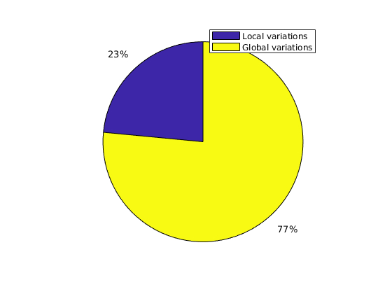
IGEMS Data Set¶

Generated from trappingIGEMS.m

The IGEMS project studied how top surface morphology influences the CO2 storage capacity. Alternative top-surface morphologies were created stochastically by combining different stratigraphic scenarios with different structural scenarios. In this example, we will use one of the top surfaces developed in the project to demonstrate capacity estimates and spill-point analysis on a model with a huge number of cells. For depositional features, two scenarios were chosen for which it was considered likely that a depositional/erosional topography could be preserved under a thick regional seal; the latter commonly formed by marine shale. The two scenarios reflect situations where sand deposition is suceeded by deposition of fines as a result of marine transgression:

In this example, we will consider an OSS-type surface that consists of sand dunes with amplitude up to 20 meters, width 2-4 km, and length 10-60 km, and spacing 2-4 km. In addition, there is a conceptual structural scenario that consists of a single fault system with random 20-150 m displacement, random 300-6000 m length, and 90 degrees strike. More information about IGEMS Link: http://www.nr.no/nb/IGEMS Data description: http://files.nr.no/igems/data.pdf

mrstModule add co2lab

Read and prepare grid structure¶

The project developed both full 3D grid saved in the ECLIPSE format and surfaces saved in the IRAP formate. The ECLIPSE files are huge (588 MB) and reading and processing them typically requires a computer with at least 12 GB memory. Here, we will therefore only use the surface grid.

Gt = topSurfaceGrid( readIGEMSIRAP('OSSNP1', 1) );

First study: geometric analyisis of caprock (spill point analysis)¶

The following command carries out a structural trapping analysis based on the geometry of the top surface. It identifies all traps (local pockets), along with their depth (at which they ‘spill over’), connections (i.e., when a trap spills over, which trap(s) does the CO2 flow into next), as well as the rivers along which CO2 flows between traps. In addition, each cell in the top surface grid is associated with an unique spill region associated with a trap (or with the exterior). A spill region of a given trap consists of all the cells in the grid that ‘leads into’ the trap; in other words, it consists of all the cells from which a quantity of CO2 would eventually flow into the trap.

ts = trapAnalysis(Gt, false); % 'true' runs a cell-based algorithm for analysis;
                              % 'false' a node-based one (but result still
                              % presented for cells, not nodes).

The resulting structure contains the following fields:

ts %#ok

ts =

  struct with fields:

           traps: [180000×1 double]
          trap_z: [99×1 double]
    trap_regions: [180000×1 double]
...


          `ts.traps` associates an integer to each cell of the top grid.  For cells located within a trap, the integer will be the index of that trap.  For other cells, the integer will be a zero.  Traps are indexed from 1 and upwards. The total number of traps would thus be given by:

num_traps = max(ts.traps) %#ok

num_traps =

    99

To have an idea about the location and distribution of traps, we can plot the trap cells on the grid by generating a scalar field over the grid cells, with two possible values (‘trap-cell’ and ‘non-trap-cell’) and then call the ‘plotCellData’ command. On the resulting plot, we can see several long-narrow traps aligned with the crests of the surface, as well as a large number of scattered, small pockets.

figure; p = get(gcf,'Position'); set(gcf,'Position', p + [0 -300 0 300]);
trap_field = zeros(size(ts.traps));
trap_field(ts.traps>0) = 2;
plot_opts = {'EdgeColor', 'k', 'EdgeAlpha', 0.1};
plotCellData(Gt, trap_field, plot_opts{:});
view(-65,25); axis tight, colormap('jet');

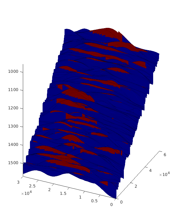
Likewise, the ‘rivers’ exiting each trap (and then either entering another trap or exiting the domain) are stored in ts.cell_lines. We can visualise them together with the traps by making a separate scalar field for rivers:

river_field = zeros(size(ts.traps));
for r = [ts.cell_lines{:}]'
    for c = 1:numel(r);
        river_field(r{c}) = 1;
    end
end

clf;
plot_opts = {'EdgeColor','none'};
plotCellData(Gt, max(trap_field, river_field), plot_opts{:});
view(-90,90); axis equal tight

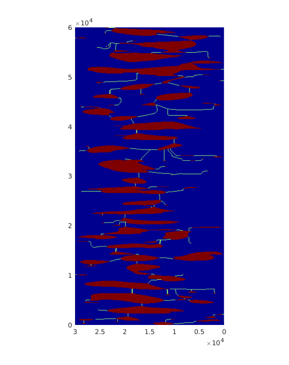
The vector ts.trap_z contains the spill point depth for each trap, i.e., the depth at which the trap ‘spills over’. The trapping capacity of a trap is thus limited to the volume between the top of the grid within that trap and the plane defined by z equal to the spill point depth of that trap. (In addition, one would have to multiply by the rock porosity, since the storage volume is limited to the pore volume.) With ts.traps, ts.trap_z and the porosity values from our averaged rock structure, we can now easily compute the storage volumes for each trap.

poro = .2*ones(Gt.cells.num,1);
trap_volumes = volumesOfTraps(Gt, ts, 1:num_traps, 'poro', poro);

total_trapping_capacity = sum(trap_volumes);
fprintf('Total trapping capacity is: %6.2e\n\n', total_trapping_capacity);

Total trapping capacity is: 5.68e+08

We can get some information on the 10 largest traps of the grid:

[sorted_vols, sorted_ix] = sort(trap_volumes, 'descend');

fprintf('trap ix   | trap vol(m3)  | cells in trap\n');
fprintf('----------+---------------+--------------\n');
for i = 1:10
   fprintf('%7d   |  %10.3e   | %5d\n', ...
       sorted_ix(i), sorted_vols(i), numel(find(ts.traps == sorted_ix(i))));
end
fprintf(['\nTogether, these traps cover %6.2e m3, which represents %3.1f ' ...
   'percent of\nthe total trapping capacity of this grid.\n'], ...
   sum(sorted_vols(1:10)), sum(sorted_vols(1:10)) / total_trapping_capacity * 100)

trap ix   | trap vol(m3)  | cells in trap
----------+---------------+--------------
     53   |   6.873e+07   |  2013
     85   |   5.091e+07   |  3166
     89   |   4.481e+07   |  1795
     98   |   3.872e+07   |  1174
     14   |   3.476e+07   |  2070
     10   |   3.239e+07   |  1570
...

Now, we visualise the location of these 10 traps (plotted in red, against the remaining traps in yellow):

largest_traps_field = zeros(size(ts.traps));
largest_traps_field(ismember(ts.traps, sorted_ix(1:10))) = 3;
clf;
plotCellData(Gt, max(trap_field, largest_traps_field), plot_opts{:});
view(-90,90);axis equal tight

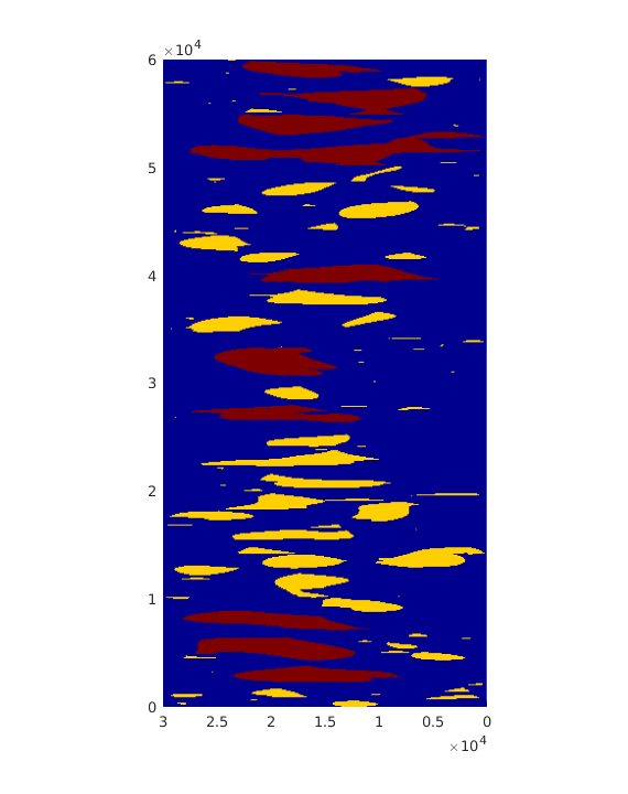
We can also color code each trap according to the total volume it holds:

for i = 1:num_traps
    trap_field(ts.traps == i) = trap_volumes(i);
end
clf;
plotCellData(Gt, trap_field, plot_opts{:});
axis equal tight; view(-90,90); colorbar;

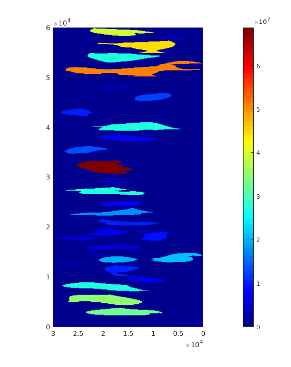
Each trap has an associated accumulation region, which consists of all cells ‘spilling into’ that trap. In other words, injection of a quantity of CO2 into one of these cells would, assuming a purely gravity-driven flow, lead it to flow into the trap. If we also count all cells leading out of the grid as a separate accumulation region, then any grid cell belongs to exactly one accumulation region (either into a specific trap or out of the domain. The accumulation region a cell belongs to is given by ts.trap_regions. There is one integer value per cell, either indicating the index of the corresponding trap, or ‘0’ if it belongs to the accumulation region that leads out of the grid domain. We can visualize these regions by plotting them as a field on the grid, and use a colormap with sharp variations in color:

clf; plotCellData(Gt, ts.trap_regions, trap_field==0,plot_opts{:});
plotGrid(Gt, trap_field>0, 'FaceColor', 'k', 'EdgeColor','none');
nreg = max(ts.trap_regions);
colormap((colorcube(nreg+1)+2*ones(nreg+1,3))/3);
view(-90,90); axis equal tight

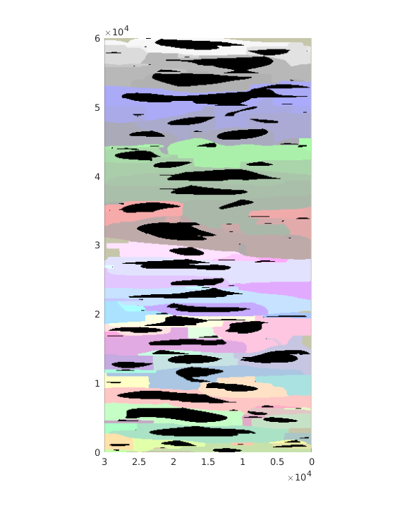
Inspect the Hugin West Formation¶

Generated from trapsHuginWest.m

This formation has the largest difference in the trap volumes. We extract a subset in the south of the model and compare the traps computed by the node-based and the cell-based algorithms

mrstModule add libgeometry opm_gridprocessing coarsegrid
grdecl = getAtlasGrid('Huginfmwest');
try
   G = processgrid(grdecl{1}); clear grdecl;
   G = mcomputeGeometry(G(1));
catch
   G = processGRDECL(grdecl{1}); clear grdecl;
   G = computeGeometry(G(1));
end

Show the whole formation with trapping structure¶

Gt = topSurfaceGrid(G);
interactiveTrapping(Gt, 'method', 'node', 'light', true, 'spillregions', true);
set(gca,'Position',[.075 .075 .85 .85])
view(-70,55)
axis on
set(gca,'XMinorGrid', 'on', 'YMinorGrid', 'on', 'ZMinorGrid', 'on', ...
   'YTickLabel',[],'XTickLabel',[]);

Current positition is not downstream from any trap, or spillpoint data was not produced.

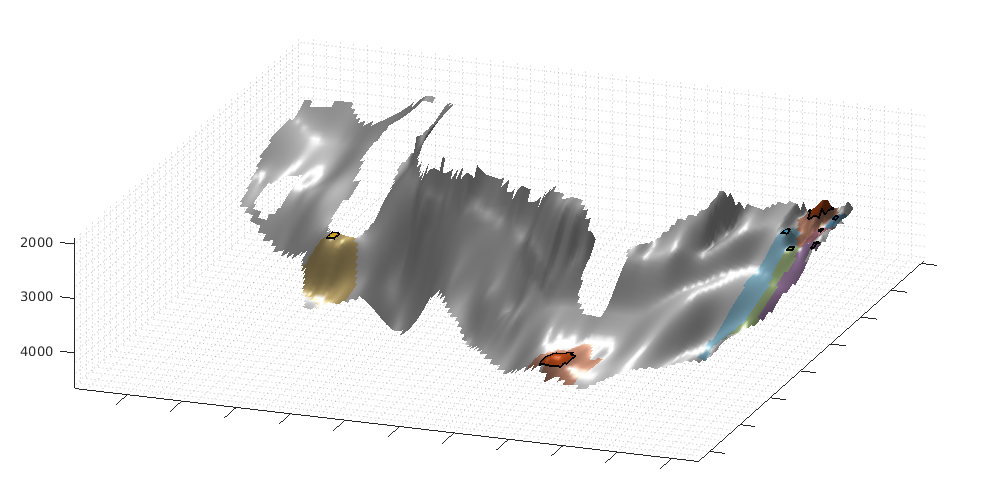
Extract a subset¶

cDims = G.cartDims;
cntrd = G.cells.centroids;
G     = extractSubgrid(G, find((cntrd(:,1) > 4.35e5) & (cntrd(:,2)<6.45e6)));
G.cartDims = cDims;
Gt = topSurfaceGrid(G);
clear cntrd cDims;

% Initialize plotting
clf;
fcol   = get(gcf,'Color');
map    = (1*hsv(6) + 1.5*repmat(fcol, 6, 1))./2.5;
map    = map([1 1:end],:); map(1,:) = fcol;
p      = get(gcf,'Position'); set(gcf,'Position', [p(1:2) 840 420]);

Node-based traps¶

Find traps using the node-based algorithms. To get a consistent ordering between the two algorithms, we use a perturbation vector to renumber the traps, from back to front in the plot.

ta  = trapAnalysis(Gt, false);
pn  = [0 5 2 3 6 1 4]';
[~, pn_inv] = sort(pn);
val = ta.trap_regions;

% Plot accumulation regions
subplot(1,2,1); cla
h   = plotCellData(Gt, ones(Gt.cells.num,1),'EdgeColor', 'none');
%set(h, 'FaceVertexCData', map(pn(val+1)+1,:));
set(h, 'FaceVertexCData', map(pn_inv(val+1),:));

% Plot traps
%plotCellData(Gt, pn(ta.traps+1), (ta.traps ~= 0), 'EdgeColor', 'k')
plotCellData(Gt, pn_inv(ta.traps+1)-1, (ta.traps ~= 0), 'EdgeColor', 'k')

% Fix axis, set light and colorbar
view(-20,40); axis tight
light('Position',[-1 -1 -1],'Style','infinite');lighting phong
colormap(hsv(6));
colorbar('horiz'); caxis([.5 6.5]);
set(gca,'XTickLabel',[],'YTickLabel',[]);

% Make table with the number of traps and corresponding volumes as computed
% by the node-based algorithm
tcn = accumarray(ta.traps+1,1);
tvn = volumesOfTraps(Gt,ta,1:6);
fprintf('\n\nNode-based method:\n');
fprintf('Trap     ');  fprintf('& %7d ', 1:6); fprintf('\\\\\\hline\n');
fprintf('Cells    '); fprintf('& %7d ', tcn(pn(2:end)+1)); fprintf('\\\\\n');
fprintf('Volume   '); fprintf('& %4.1e ',tvn(pn(2:end))); fprintf('\\\\\\hline\n\n');

Node-based method:
Trap     &       1 &       2 &       3 &       4 &       5 &       6 \\\hline
Cells    &       1 &       2 &       2 &      18 &       2 &       1 \\
Volume   & 5.5e+06 & 3.5e+06 & 1.8e+07 & 3.9e+08 & 2.4e+07 & 5.8e+06 \\\hline

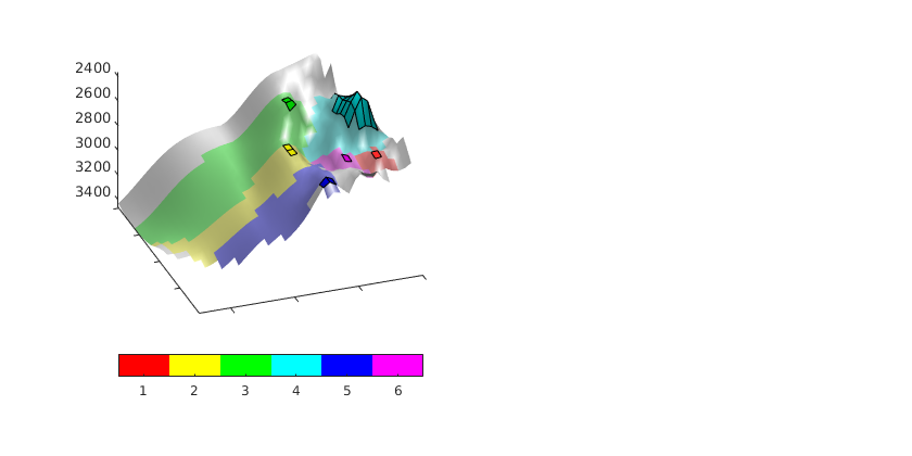
Cell-based traps¶

Find traps using the node-based algorithms. To get a consistent ordering between the two algorithms, we use a perturbation vector to renumber the traps, from back to front in the plot.

ta  = trapAnalysis(Gt, true);
%pc  = [0 1 4 2 5 3 6]';
pc  = [0 1 3 5 2 4 6]';
[~, pc_inv] = sort(pc);
val = ta.trap_regions;

% Plot accumulation regions
subplot(1,2,2); cla
h   = plotCellData(Gt, ones(Gt.cells.num,1), 'EdgeColor', 'none');
%set(h, 'FaceVertexCData', map(pc(val+1)+1,:));
set(h, 'FaceVertexCData', map(pc_inv(val+1),:));

% Plot traps
%plotCellData(Gt, pc(ta.traps+1), (ta.traps ~= 0), 'EdgeColor', 'k')
plotCellData(Gt, pc_inv(ta.traps+1)-1, (ta.traps ~= 0), 'EdgeColor', 'k')

% Fix axis, set light and colorbar
view(-20,40); axis tight
light('Position',[-1 -1 -1],'Style','infinite');lighting phong
colorbar('horiz'); caxis([.5 6.5]);
set(gca,'XTickLabel',[],'YTickLabel',[]);

% Make table with the number of traps and corresponding volumes as computed
% by the cell-based algorithm
tcc = accumarray(ta.traps+1,1);
tvc = volumesOfTraps(Gt,ta,1:6);
fprintf('\n\nCell-based method:\n');
fprintf('Trap     '); fprintf('& %7d ', 1:6); fprintf('\\\\\\hline\n');
fprintf('Cells    '); fprintf('& %7d ', tcc(pc(2:end)+1)); fprintf('\\\\\n');
fprintf('Volume   '); fprintf('& %4.1e ',tvc(pc(2:end))); fprintf('\\\\\\hline\n\n');

Loading module matlab_bgl
Trap level 1: 6 traps identified
Warning: purging 1 bad traps with 0 spill value.
Start find rivers


Cell-based method:
Trap     &       1 &       2 &       3 &       4 &       5 &       6 \\\hline
...

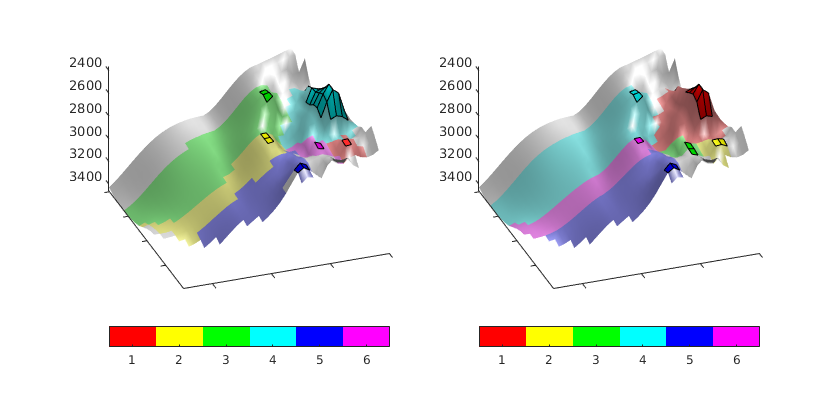
Trapping on Johansen grids¶

Generated from trapsJohansen.m

The Johansen formation has been proposed as a potential injection site for CO2, in particular when it was planned to capture CO2 from the gas-power plant at Mongstad. A simplified representation of the Johansen formation was also used as a benchmark case in the Stuttgart code comparison study based on a paper by Eigestad et al. Herein, we consider the same injection point as suggested by Eigestad et al. and evaluate the potential for structural trapping that can be estimated from two different models: (i) a sector model developed by the Norwegian Petroleum Directorate, which was used to produce the Stuttgart benchmark test, and (ii) a model of a somewhat larger region derived from the CO2 Storage Atlas for the Norwegian North Sea.

mrstModule add co2lab libgeometry opm_gridprocessing coarsegrid matlab_bgl

Load NPD data: sector model¶

try
   jdir = fullfile(mrstPath('co2lab'), 'data', 'johansen');
   sector = 'NPD5';
   sector = fullfile(jdir, sector);
   grdecl = readGRDECL([sector '.grdecl']);
catch me
   disp(' -> Download data from: http://www.sintef.no/Projectweb/MatMoRA/')
   disp(['    Putting data in ', jdir]);
   unzip('https://www.sintef.no/project/MatMoRA/Johansen/NPD5.zip', jdir);
   grdecl = readGRDECL([sector '.grdecl']);
end

% Extract the part that represents the Johansen formation
grdecl = cutGrdecl(grdecl,[1 grdecl.cartDims(1); 1 grdecl.cartDims(2);  6 11]);
try
   Gs = processgrid(grdecl);
   Gs = mcomputeGeometry(Gs);
catch
   Gs = processGRDECL(grdecl);
   Gs = computeGeometry(Gs);
end

Gts = topSurfaceGrid(Gs);

% Get the position of the well (data given from 'Sector5_Well.txt');
wi    = find(Gs.cells.indexMap==sub2ind(Gs.cartDims, 48, 48, 1));
wcent = Gs.cells.centroids(wi,:);
d = sqrt(sum(bsxfun(@minus, Gts.cells.centroids, wcent(1:2)).^2, 2));
[~,wi_s] = min(d);

Warning: Could not add face tags. 3D grid G has no regular cell.

Load NPD data: full-field model¶

try
   jdir = fullfile(mrstPath('co2lab'), 'data', 'johansen');
   sector = 'FULLFIELD_IMAXJMAX';
   sector = fullfile(jdir, sector);
   grdecl = readGRDECL([sector '.GRDECL']);
catch me
   disp(' -> Download data from: http://www.sintef.no/Projectweb/MatMoRA/')
   disp(['    Putting data in ', jdir]);
   unzip('https://www.sintef.no/project/MatMoRA/Johansen/FULLFIELD_Eclipse.zip', jdir);
   grdecl = readGRDECL([sector '.GRDECL']);
end

% Extract the part that represents the Johansen formation
grdecl = cutGrdecl(grdecl,[1 grdecl.cartDims(1); 1 grdecl.cartDims(2);  10 14]);
try
   Gf = processgrid(grdecl);
   Gf = mcomputeGeometry(Gf);
catch
   Gf = processGRDECL(grdecl);
   Gf = computeGeometry(Gf);
end
Gtf = topSurfaceGrid(Gf);

% Get the position of the well
d = sqrt(sum(bsxfun(@minus, Gtf.cells.centroids, wcent(1:2)).^2, 2));
[~,wi_f] = min(d);

Warning: Degenerate edges in 3D grid has led to adjacent cells in 2D grid that
should not be considered neighbors.
Warning: Could not add face tags. 3D grid G has no regular cell.

Load atlas data¶

grdecl = getAtlasGrid('Johansenfm');
try
   Ga = processgrid(grdecl{1});
   Ga = mcomputeGeometry(Ga);
catch
   Ga = processGRDECL(grdecl{1});
   Ga = computeGeometry(Ga);
end
Gta = topSurfaceGrid(Ga);

% Get the position of the well
d = sqrt(sum(bsxfun(@minus, Gta.cells.centroids, wcent(1:2)).^2, 2));
[~,wi_a] = min(d);

Plot the three data sets¶

clf
zm = min(Ga.nodes.coords(:,3));
zM = max(Ga.nodes.coords(:,3));

plotCellData(Ga,Ga.cells.centroids(:,3),'FaceAlpha',.95,'EdgeColor','none');
plotGrid(Gf,'FaceColor','none','EdgeAlpha',.2,'EdgeColor','r');
plotGrid(Gs,'FaceColor','none','EdgeAlpha',.4,'EdgeColor','k');
axis tight, view(-62,60);
light, lighting phong,
light('Position',[max(Gta.cells.centroids) 4*zM],'Style','infinite');

hold on; plot3(wcent([1 1],1),wcent([1 1],2),[zm zM],'b','LineWidth',2);

legend('Atlas','Full field','Sector','Inj.pt',...
   'Location','SouthOutside','Orientation','horizontal');

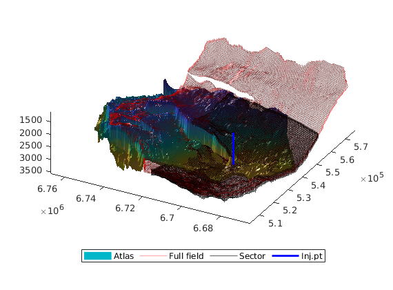
Interactive trapping: atlas grid¶

interactiveTrapping(Gta, 'method', 'cell', 'light', true, ...
   'spillregions', true, 'colorpath', false, 'injpt', wi_a);
view(-80,64);

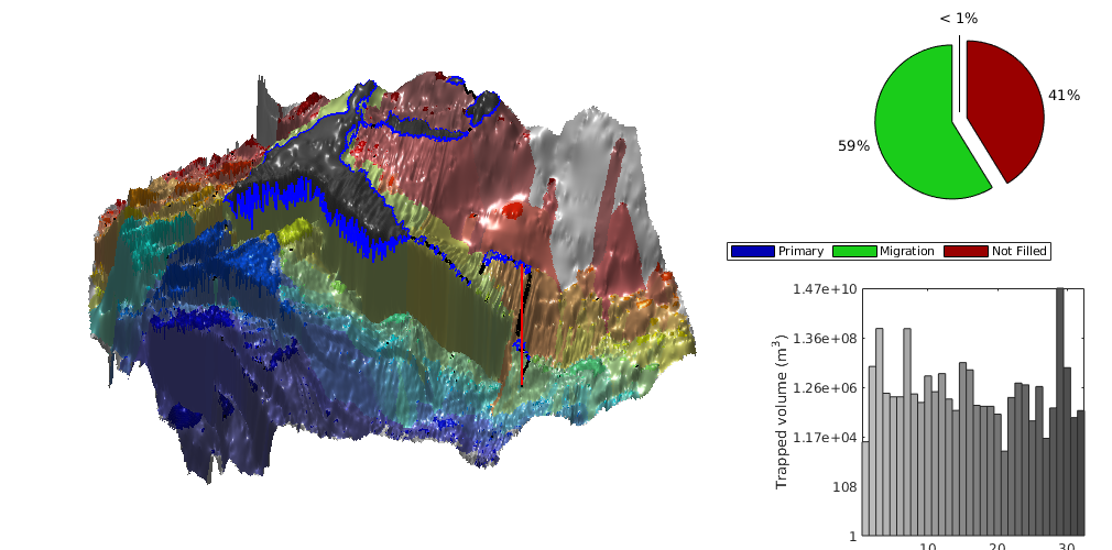
Interactive trapping: NPD sector grid¶

interactiveTrapping(Gts, 'method', 'cell', 'light', true, ...
   'spillregions', true, 'colorpath', false, 'injpt', wi_s);
view(-80,64);

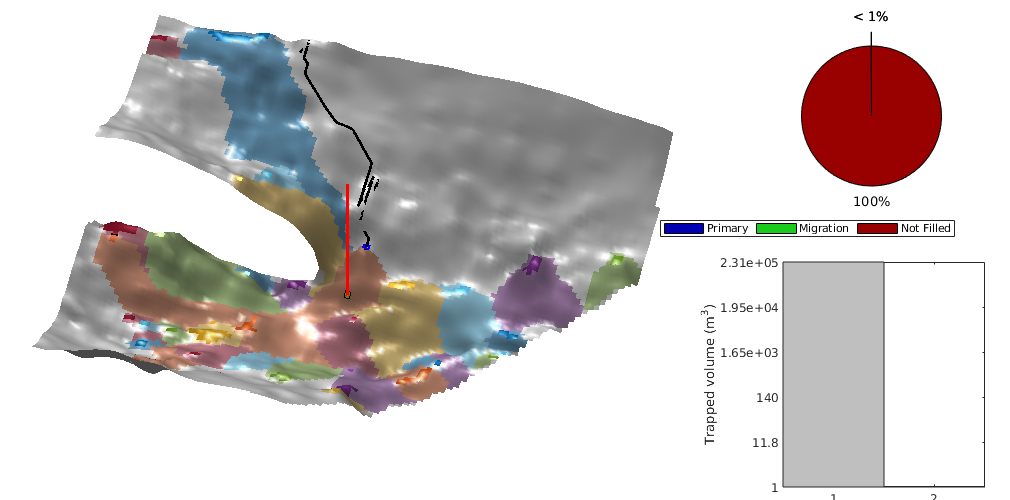
Interactive trapping: NPD full-field grid¶

interactiveTrapping(Gtf, 'method', 'cell', 'light', true, ...
   'spillregions', true, 'colorpath', false, 'injpt', wi_f);
view(-80,64);

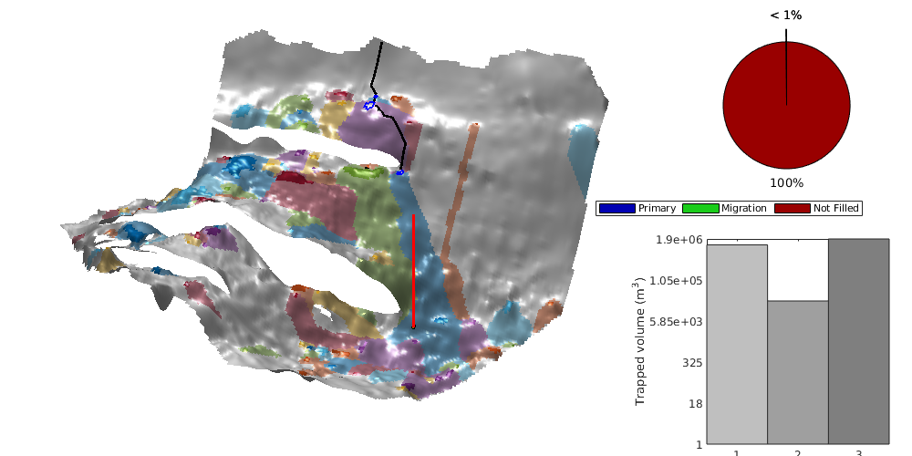
Brine Production Example¶

Generated from brineProductionExample.m

In this example, we use a simple well configuration in the Bjarmeland formation (Barents Sea) to demonstrate the use of brine production for enhancing storage capacity. Injection and production controls are optimized according to an objective function which penalizes leakage and pressure-buildup (as done in ‘pressureLimitedExample.m’).

mrstModule add ad-core ad-props optimization
gravity on;

saveResults = false;

Set-up model and perform initial simulation¶

[model, schedule, initState, seainfo, other] = setupProdExModel( ...
    'itime', 10*year,   'isteps',5,  ...
    'mtime', 100*year,  'msteps',10  );

Loading module libgeometry
Warning: Nan permeability values are being replaced with the average value.
Warning: Nan porosity values are being replaced with the average value.
Warning: Nan net-to-gross values are being replaced with the average value.
Loading module matlab_bgl
Loading module coarsegrid
Trap level 1: 26 traps identified
Trap level 2: 6 traps identified
...

Initial simulation:

[init.wellSols, init.states] = simulateScheduleAD(initState, model, schedule, ...
                             'NonLinearSolver', NonLinearSolver('useRelaxation', true));
init.schedule = schedule;

%sameControlTypes = all(strcmpi({schedule.control(1).W.type}, {schedule.control(2).W.type}));

Solving timestep 01/15:           -> 2 Years
Solving timestep 02/15: 2 Years   -> 4 Years
Solving timestep 03/15: 4 Years   -> 6 Years
Solving timestep 04/15: 6 Years   -> 8 Years
Solving timestep 05/15: 8 Years   -> 10 Years
Solving timestep 06/15: 10 Years  -> 20 Years
Solving timestep 07/15: 20 Years  -> 30 Years
Solving timestep 08/15: 30 Years  -> 40 Years
...

Define some parameters¶

We use a leakage penalty factor of 5. We set the pressure limit to be 90% of the overburden pressure, and the pressure penalty factors will be gradually ramped up until the optimal solution is one in which the pressure limit is surpassed within a tolerance of 2%.

P_over      = computeOverburdenPressure(model.G, model.rock, seainfo.seafloor_depth, model.fluid.rhoWS);
p_lim_fac   = 0.9;
P_limit     = P_over * p_lim_fac;
cP          = [1e-9, 1e-8, 1e-7, 1e-6, 1e-5, 1e-4, 1e-3, 1e-2, 1e-1]; % pressure penalty factor
cL          = 5; % leakage penalty factor

Evaluate initial objective (using lowest cP):¶

Our objective is to maximize CO2 storage while minimizing long-term leakage and pressure buildup. See ‘pressureLimitedExample.m’ for more details on this objective function.

obj_funA = @(wellSols, states, schedule, varargin) ...
            leakPenalizerAtInfinity(model, wellSols, states, ...
                schedule, cL, other.surface_pressure, ...
                model.fluid.rhoWS, other.ta, varargin{:});
obj_funB = @(states, varargin) ...
            pressurePenalizer(model, states, schedule, cP(1), ...
                P_limit, varargin{:});

% We scale the initial objective using obj_funA since obj_funB can be very
% large if the initial guess caused the pressure limit to be greatly
% surpassed.
init.obj_val_steps_A = cell2mat( obj_funA(init.wellSols, init.states, init.schedule) );
init.obj_val_steps_B = cell2mat( obj_funB(init.states) );
init.obj_val_steps = init.obj_val_steps_A - init.obj_val_steps_B;
init.obj_val_total = sum(init.obj_val_steps);
%obj_scaling = abs(init.obj_val_total);
obj_scaling = abs( sum(init.obj_val_steps_A) );

init0 = init; % keep the initial simulation results

Loading module ad-blackoil
Total injected: 67834123.969208 (m3)
Total leaked (by infinity): -8.034761 (m3)
Penalty: 5.000000
Score: 67834164.143011 (m3)

Surpassed Plimit by 0.000000 (percent) of Plimit.
Approached Plimit by 4.495609 (percent) of Plimit.

Define min and max well control values (used to set up box limits)¶

Here, we set the limits for the injector wells to be “zero” and some multiple of the highest injector rate. The producer wells are limited to operate between 50 bars and the initial hydrostatic pressure near the well.

% schedule indexes for 'rate' (injector) and 'bhp' (producer) control wells
injWinx = find(strcmpi({schedule.control(1).W.type},'rate'));
prdWinx = find(strcmpi({schedule.control(1).W.type},'bhp'));
prdWcel = [schedule.control(1).W(prdWinx).cells];

% well control limits for injection period
min_wvals( injWinx ) = sqrt(eps);                                       % min well value for injectors, m3/s
min_wvals( prdWinx ) = 50*barsa;                                        % min well value for producers, Pascal
max_wvals( injWinx ) = 3*max([schedule.control(1).W( injWinx ).val]);   % max well value for injectors, m3/s
max_wvals( prdWinx ) = initState.pressure( prdWcel );                   % max well value for producers, Pascals

Loop through pressure penalty factors until convergence reached within¶

tolerance of 2% of P_limit

sch = schedule;
for r = 1:numel(cP)
    cP_curr = cP(r);

    % Must re-define pressure penalizer with current penalty factor
    obj_funB = @(states, varargin) ...
                pressurePenalizer(model, states, sch, cP_curr, ...
                    P_limit, varargin{:});

    obj_fun = @(wellSols, states, schedule, varargin) ...
                cellSubtract(  obj_funA(wellSols, states, schedule, varargin{:}), ...
                    obj_funB(states, varargin{:})   );


    % Optimize injection rates using the BFGS optimization algorithm.
    % Passing in 'obj_scaling' means an initial simulation will not be
    % executed by optimizeRates. The initial schedule is as per 'sch'.
    [optim, init, history] = optimizeControls(initState, model, sch, min_wvals, max_wvals, ...
                                'obj_fun',                      obj_fun, ...
                                'last_control_is_migration',    true, ...
                                'obj_scaling',                  obj_scaling, ...
                                'lineSearchMaxIt',              5, ...
                                'gradTol',                      1e-3, ...
                                'objChangeTol',                 1e-3);


    % Decide whether to ramp up cP or whether convergence reached
    [~, perc_of_Pover_reach] = ...
        findMaxPercentagePlimitReached( optim.states, P_limit, P_over );

    if (perc_of_Pover_reach/100 - p_lim_fac) > 0.02
        % use optimized rates as next iteration's initial rates
        sch = optim.schedule;
        % NB: init_scale won't reduce these rates
        % NB: max_wvals won't be in terms of these rates
    elseif r == numel(cP)
        warning('Convergence did not occur before or using last pressure penalty factor.')
    else
        % open system: if p < (plim + tolerance), optimal rates found
        break % exit cp(r) loop
    end

end

Solving timestep 01/15:           -> 2 Years
Solving timestep 02/15: 2 Years   -> 4 Years
Solving timestep 03/15: 4 Years   -> 6 Years
Solving timestep 04/15: 6 Years   -> 8 Years
Solving timestep 05/15: 8 Years   -> 10 Years
Solving timestep 06/15: 10 Years  -> 20 Years
Solving timestep 07/15: 20 Years  -> 30 Years
Solving timestep 08/15: 30 Years  -> 40 Years
...

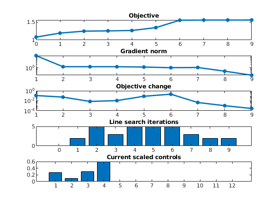
Saving¶

add variables to ‘other’, used for post-processing

other.fluid = model.fluid;
other.initState = initState;
other.leak_penalty = cL;
Gt = model.G;

if saveResults
    dirName = 'brineProductionExampleResults';
    mkdir(dirName);
    save(fullfile(dirName, 'Gt'),       'Gt');
    save(fullfile(dirName, 'optim'),    'optim');
    save(fullfile(dirName, 'init0'),    'init0');
    save(fullfile(dirName, 'init'),     'init');
    save(fullfile(dirName, 'history'),  'history');
    save(fullfile(dirName, 'other'),    'other'); % @@ fluid structure is quite large
end

VE simulation in a standard black-oil solver¶

Generated from exampleVEBlackOilAD.m

In this example we show how to set up a standard format black-oil model that can be used to simulate a VE model. For the actual simulation, we use the fully-implicit solver in MRST, based on automatic differentiation.

mrstModule add co2lab ad-props deckformat ad-core ad-blackoil

Parameters for the simulation¶

gravity on
[nx,ny,nz] = deal(40, 1, 1);     % Cells in Cartsian grid
[Lx,Ly,H]  = deal(2000,1000,15); % Physical dimensions of reservoir
total_time = 5*year;             % Total simulation time
nsteps     = 10;                 % Number of time steps in simulation
dt         = total_time/nsteps;  % Time step length
perm       = 100;                % Permeability in milli darcies
phi        = 0.1;                % Porosity
depth      = 1000;               % Initial depth
ipress     = 200;                % Initial pressure

Create input deck and construct grid¶

Create an input deck that can be used together with the fully-implicit black oil solver. Since the grid is constructed as part of setting up the input deck, we obtain it directly.

deck = sinusDeckAdiVE([nx, ny, nz], [Lx, Ly, H], nsteps, dt, ...
                      -.1*pi/180, depth, phi, perm, ...
                      (H*phi*Lx*Ly)*0.2*day/year, ipress);

deck = convertDeckUnits(deck);

Initialize data structures¶

[x0, model, schedule] = initEclipseProblemAD(deck);

Warning: Reference depth for well BHP in well 'P01' is set below well's top-most
reservoir connection
Warning: Reference depth for well BHP in well 'P01' is set below well's top-most
reservoir connection

Show simulation grid¶

This is stored as the G data member of the simulation model.

figure, plotGrid(model.G), view([0, -1, 0]), box on

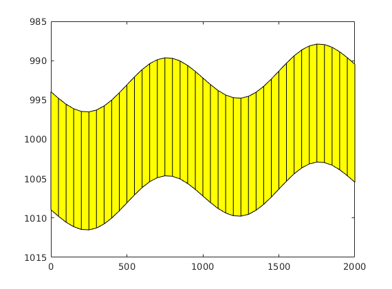
Prepare simulation model, schedule and initial state¶

Before we can run the simulation, we make sure that we have an initial hydrostatic pressure distribution. We proceed by creating a simulation model object that the solver can work with, representing a two-phase oil/water system, where we let ‘oil’ represent the CO2 phase. Finally, we convert the schedule from the input deck into MRST format.

z  = model.G.cells.centroids(:,3);
x0.pressure = ipress*barsa +(z(:)-z(end))*norm(gravity)*deck.PROPS.DENSITY(2);
x0.sGmax = x0.s(:,2);

Run the schedule setup in the file¶

Before we can run the schedule, we make sure that we have an initial hydrostatic pressure distribution. Then we pick the schedule from the input deck and start the simulator.

[wellSols, states] = simulateScheduleAD(x0, model, schedule);

Solving timestep 01/10:         -> 182 Days, 12 Hours
Solver did not converge in 25 iterations for timestep of length 182 Days, 12 Hours. Cutting timestep.
Solver did not converge in 25 iterations for timestep of length 91 Days, 6 Hours. Cutting timestep.
Solving timestep 02/10: 182 Days, 12 Hours -> 1 Year
Solving timestep 03/10: 1 Year  -> 1 Year, 182 Days, 12.00 Hours
Solving timestep 04/10: 1 Year, 182 Days, 12.00 Hours -> 2 Years
Solving timestep 05/10: 2 Years -> 2 Years, 182 Days, 12.00 Hours
Solving timestep 06/10: 2 Years, 182 Days, 12.00 Hours -> 3 Years
...

Plot results¶

%figure
Gt = topSurfaceGrid(model.G);
xc = Gt.cells.centroids(:,1);
zt = Gt.cells.z;
zb = zt + Gt.cells.H;
for nn=1:numel(states)
    clf
    state=states{nn};

    subplot(2,2,1),cla
    title('pressure')
    plotCellData(model.G,convertTo(state.pressure,barsa),'EdgeColor','none');
    colorbar('horiz'), caxis([100 200])

    subplot(2,2,2),cla
    title('saturation')
    plotCellData(model.G,state.s(:,1),'EdgeColor','none');
    colorbar('horiz'), caxis([0 1])

    % plot as VE
    subplot(2,2,3),cla
    plot(xc,convertTo(state.pressure,barsa)); set(gca,'YLim',[100 200]);

    subplot(2,2,4),cla,hold on
    patch(xc([1 1:end end]), [zt(end)-10; zt; zt(end)-10],.7*[1 1 1]);
    patch(xc([1 1:end end]), [zb(end)+10; zb; zb(end)+10],.7*[1 1 1]);
    patch(xc([1:end end:-1:1]), ...
      [zt + Gt.cells.H.*state.s(:,2); zt(end:-1:1)], getVEColors('plume'))
    patch(xc([1:end end:-1:1]), ...
      [zt + Gt.cells.H.*state.s(:,2); zb(end:-1:1)], getVEColors('brine'))
    set(gca,'YDir','reverse'), axis tight

    drawnow;
    pause(0.01)
end

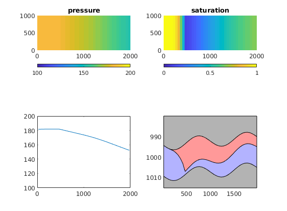
Examples to demonstrate forecast of CO2 leakage and its application¶

Generated from leakageForecastDemo.m

By assuming a system’s flow dynamics are gravity-dominated, we determine the amount of CO2 remaining in the domain using spill-point dynamics.

mrstModule add co2lab

1. Synthetic grid¶

For simplicity, we first consider a synthetic grid of a sloping and perturbed topsurface. Beginning with a domain that is fully saturated with CO2, the forecast amount of CO2 remaining is shown to be equivalent to the structural trapping capacity (in the event that there is no residual trapping). On the other hand, when residual trapping is included, the forecast amount remaining is a conservative estimate (since we do not forecast the areal sweep of the plume as it migrates), but this estimate is shown to be close to the structural and residual trapping capacity.

% Getting grid and rock:
Gt = dippedPerturbedGrid();
rock2D.poro = ones(Gt.cells.num,1) * 0.25;
rock2D.perm = ones(Gt.cells.num,1) * 500 * milli*darcy;

Trap analysis: labeling trap and catchment numbers

figure; hold on
ta = trapAnalysis(Gt, true);
plotGrid(Gt, 'facecolor','none', 'edgealpha',0.1);
colorizeCatchmentRegions(Gt, ta);
num_traps = numel((unique(ta.traps(ta.traps ~= 0))));
for i = 1:num_traps
    trapcells = find(ta.traps==i);
    plotCellData(Gt, ones(Gt.cells.num,1).*i, trapcells, ...
        'facecolor',[0.5 0.5 0.5], 'facealpha',0.5, 'edgecolor','none');
end
top = topCellOfTrap(Gt, ta);
[x, y] = deal(Gt.cells.centroids(top,1), Gt.cells.centroids(top,2));
data = 1:1:numel(top);
data = data';
text(x, y, Gt.cells.z(top)-3, cellstr(num2str(data, '%3.0f')), ...
   'HorizontalAlignment','center', 'FontSize',16, 'FontWeight', 'bold');
axis tight off; view([42,48])

Loading module matlab_bgl
Loading module coarsegrid
Trap level 1: 6 traps identified
Start find rivers

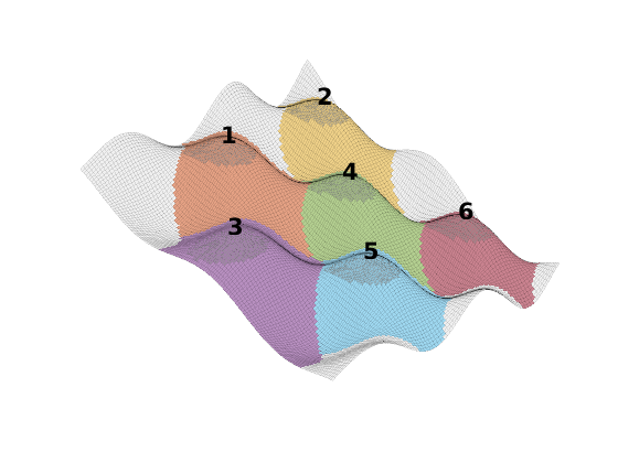
Fluid model

seainfo = getSeaInfo('NorthSea',760);
%seainfo.res_sat_wat = 0; % @@ can use for testing
%seainfo.res_sat_co2 = 0; % @@ can use for testing
T_ref = computeCaprockTemperature(Gt, seainfo.seafloor_temp, ...
    seainfo.seafloor_depth, seainfo.temp_gradient);
T_ref = T_ref + 273.15; % Kelvin
p     = computeHydrostaticPressure(Gt, seainfo.water_density, 1*atm);
P_ref = mean(p);
fluid = makeVEFluid(Gt, rock2D, 'sharp interface'                   , ...
       'fixedT'       , T_ref                                       , ...
       'residual'     , [seainfo.res_sat_wat  , seainfo.res_sat_co2], ...
       'wat_rho_ref'  , seainfo.water_density                       , ...
       'co2_rho_ref'  , seainfo.rhoCref                             , ...
       'wat_rho_pvt'  , [4.3e-5/barsa         , P_ref]              , ...
       'co2_rho_pvt'  , [[0.1 400]*mega*Pascal, [4 250]+274]        , ...
       'wat_mu_ref'   , seainfo.water_mu                            , ...
       'co2_mu_pvt'   , [[0.1 400]*mega*Pascal, [4 250]+274]        , ...
       'pvMult_fac'   , 1e-5/barsa                                  , ...
       'pvMult_p_ref' , P_ref                                       , ...
       'dissolution'  , false                                       , ...
       'surf_topo'    , 'smooth');

Creating a state of CO2 saturation: We assume the formation is fully saturated with CO2. If there is no residual water, then CO2 saturations will be 1, otherwise they are equal to 1-sw to account for residual water occupying the pore space.

sG    = ones(Gt.cells.num,1) .* (1 - fluid.res_water);
sGmax = sG;
sF    = ones(Gt.cells.num,1) - sG;

Using spill-point dynamics to predict future mass remaining/leaked:

mrstVerbose on;
[ will_stay, will_leak ] = massAtInfinity( Gt, rock2D, p, ...
    sG, sGmax, sF, 0, fluid, ta, [], 'plotsOn',true );

Loading module ad-core
Loading module ad-props
Loading module ad-blackoil

------------------
Initial inventory:
------------------

...

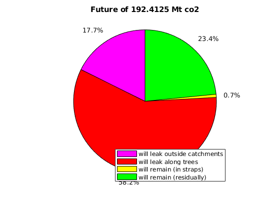
2. Injected CO2 scenario into a realistic grid¶

Here, we simulate the injection and migration of CO2 into a real formation using a vertical-equilibrium model. This example helps to show the transition from pressure-driven to gravity-dominated flow, and the impact it has on our forecasting algorithm. That is, non-monotonic behavior is noticed in the forecast curve immediately following the injection period, and several years must be simulated before the forecast curve begins to converge. However, once the forecast has converged, there is no need to simulate the migration period any further.

% Setting up (cropped) model:
[Gt, rock2D] = getFormationTopGrid('Utsirafm',3);
ind          = (max(Gt.cells.centroids(:,2)) - Gt.cells.centroids(:,2)) < 200 * kilo * meter;
[g, cellmap] = removeCells(Gt.parent, find(~ind)); clear Gt
Gt           = topSurfaceGrid(g);   clear g
rock2D.poro = rock2D.poro(cellmap);
rock2D.perm = rock2D.perm(cellmap); clear cellmap
ta               = trapAnalysis(Gt, true);
seainfo          = getSeaInfo('Utsirafm', 760);
caprock_pressure = (Gt.cells.z * seainfo.water_density * norm(gravity)) ...
                .* (1 + seainfo.press_deviation/100); % @@ should add 1*atm
P_ref = mean(caprock_pressure);
T_ref = computeCaprockTemperature(Gt, seainfo.seafloor_temp, ...
    seainfo.seafloor_depth, seainfo.temp_gradient);
T_ref = T_ref + 273.15; % Kelvin
fluid = makeVEFluid(Gt, rock2D, 'sharp interface'                   , ...
       'fixedT'       , T_ref                                       , ...
       'residual'     , [seainfo.res_sat_wat  , seainfo.res_sat_co2], ...
       'wat_rho_ref'  , seainfo.water_density                       , ...
       'co2_rho_ref'  , seainfo.rhoCref                             , ...
       'wat_rho_pvt'  , [4.3e-5/barsa         , P_ref]              , ...
       'co2_rho_pvt'  , [[0.1 400]*mega*Pascal, [4 250]+274]        , ...
       'wat_mu_ref'   , seainfo.water_mu                            , ...
       'co2_mu_pvt'   , [[0.1 400]*mega*Pascal, [4 250]+274]        , ...
       'pvMult_fac'   , 1e-5/barsa                                  , ...
       'pvMult_p_ref' , P_ref                                       , ...
       'dissolution'  , false                                       , ...
       'surf_topo'    , 'smooth');
model = CO2VEBlackOilTypeModel(Gt, rock2D, fluid);

% Defining initial state:
initState.pressure  = computeHydrostaticPressure(Gt, fluid.rhoWS, 1*atm);
initState.s         = repmat([1 0], Gt.cells.num, 1);
initState.sGmax     = initState.s(:,2);

Loading module libgeometry
Processing Utsirafm ...
Adding 55468 artificial cells at top/bottom

Processing regular i-faces
 Found 38516 new regular faces
Elapsed time is 0.024934 seconds.

...

Simulate injection and migration¶

We simulate 10 years of injection and 300 years of migration using a standard VE model.

itime  = 10 * year;
isteps = 10;
mtime  = 300 * year;
msteps = 30;
dTi         = itime / isteps;
dTm         = mtime / msteps;
istepvec    = ones(isteps, 1) * dTi;
mstepvec    = ones(msteps, 1) * dTm;
schedule.step.val       = [istepvec; mstepvec];
schedule.step.control   = [ones(isteps, 1); ones(msteps, 1) * 2];

% Setting up injection well:
wcinx = findEnclosingCell(Gt, [4.7777e5, 6.8154e6]);
W = addWell([], Gt.parent, rock2D, wcinx, ...
                'name',     ['Winj' num2str(wcinx)],  ...
                'Type',     'rate', ...
                'Val',      0.3536, ...
                'comp_i',   [0,1], ...
                'Radius',   0.3 );
W = convertwellsVE(W, Gt.parent, Gt, rock2D, 'ip_tpf');
W_shut = W;
W_shut.val = sqrt(eps);
schedule.control(1).W = W;
schedule.control(2).W = W_shut;

% Setting up boundary conditions:
bfaces  = find(any(Gt.faces.neighbors==0,2));
bdryVal = Gt.faces.z(bfaces) * fluid.rhoWS * norm(gravity) + 1*atm;
schedule.control(1).bc = addBC( [], bfaces, 'pressure', bdryVal, 'sat', [1 0] );
schedule.control(2).bc = addBC( [], bfaces, 'pressure', bdryVal, 'sat', [1 0] );

% Simulating injection and migration:
mrstVerbose off;
[wellSols, states] = simulateScheduleAD(initState, model, schedule);

Defaulting reference depth to top of formation for well Winj4495. Please specify 'refDepth' optional argument to 'addWell' if you require bhp at a specific depth.
Warning: Reference depth for well BHP in well 'Winj4495' is set below well's
top-most reservoir connection
Solving timestep 01/40:           -> 1 Year
================================================================================================
| It # | water (cell) | gas (cell) | waterWells (perf) | gasWells (perf) | closureWells (well) |
================================================================================================
|    1 | 2.95e-01     | 7.79e-03   |*0.00e+00          | 3.46e-01        |*0.00e+00            |
...

Forecast¶

For each time step in the simulation, we extract the aquifer state and use it to make a spill-point forecast of the mass that will be trapped at time infinity. We then plot the resulting curve as a blue line on top of the trapping inventory from the vertical-equilibrium simulation.

Ma = zeros(numel(states),1);
for i = 1:numel(states)
    Ma(i) = massAtInfinity( model.G, model.rock, states{i}.pressure, ...
        states{i}.s(:,2), states{i}.sGmax, states{i}.s(:,1), 0, ...
        model.fluid, ta, [] ) / 1e12; % Gt
end

% Plotting Ma on top of trapping inventory
reports = makeReports(Gt, [{initState}; states], rock2D, fluid, ...
                    schedule, [fluid.res_water, fluid.res_gas], ta, []);
h = figure;
plot(1);
ax = get(h,'currentaxes');
plotTrappingDistribution(ax, reports, 'legend_location', 'southeast');
fsize = 10;
set(get(gca, 'xlabel'), 'fontsize', fsize)
set(get(gca, 'ylabel'), 'fontsize', fsize)
set(gca,'fontsize', fsize);
hold on;
plot([0; cumsum(convertTo(schedule.step.val,year))], [0; Ma*1e3], 'b','LineWidth',3)

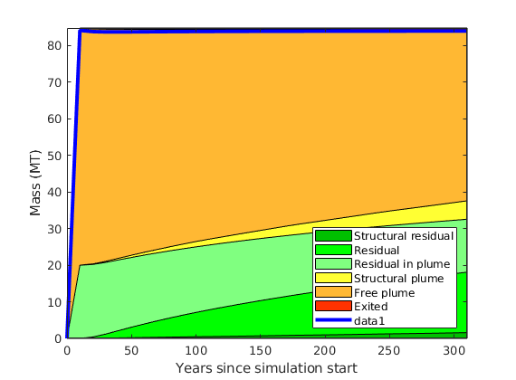
Show non-monotonicity¶

Adding stars to forecast curve corresponding to the CO2 sat. snapshots

[x,y] = deal([0; cumsum(convertTo(schedule.step.val,year))], [0; Ma*1e3]);
% x is in years, y is in Mt
for i=1:5
    plot(x(10+i), y(10+i), '*', 'MarkerSize',10, 'LineWidth',2, 'Color','k')
end

% Zooming into curve to see non-monotonicity
xlim([0 100])
ylim([83 84.738])

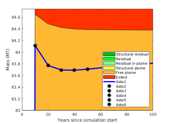
Plot snapshots of CO2 saturation¶

sts = [{initState}; states];
tol = 0.005;
time_yr = [0; convertTo(cumsum(schedule.step.val),year)];
for np = 1:5

    tinx = 10 + np; % plot "sts" corresponding to years 10, 20, 30, 40, 50

    figure; hold on
    plotGrid(Gt, 'facecolor','none', 'edgealpha',0.1)
    colorizeCatchmentRegions(Gt, ta);
    plotCellData(Gt, sts{tinx}.s(:,2), sts{tinx}.s(:,2) > tol, 'edgecolor','none')

    cmax = max(sts{tinx}.s(:,2));
    set(findobj(gcf,'type','axes'),'clim',[0, cmax])
    colormap(gca,parula)
    daspect([1 1 0.02])
    axis tight off

    % add rivers between traps
    rivers = ta.cell_lines;
    for tr = rivers
        for r = tr{:}
            drawCellConnections3D(Gt, r{:}, 'color', 'k', 'lineWidth', 2);
        end
    end

    % add traps (or just trap outlines)
    plotCellData(Gt, ones(Gt.cells.num,1), ta.traps ~= 0, ...
        'facecolor','b','facealpha',0.2, 'edgecolor','none')
    for i = 1:numel(ta.trap_z)
        plotFaces(Gt, boundaryFaces(Gt, ta.trap_regions == i), 'EdgeColor','k','LineWidth',1)
        plotFaces(Gt, boundaryFaces(Gt, ta.traps == i), 'EdgeColor','b','LineWidth',2)
    end

    % add well location
    plotWell(Gt.parent, W, 'color','k')


    title(['Year ',num2str(time_yr(tinx))])

    % getting reports for catchment regions surrounding the well
    fprintf('\n-----------\n')
    fprintf(  'By Year %d:', time_yr(tinx))
    fprintf('\n-----------\n')
    massAtInfinity( Gt, rock2D, sts{tinx}.pressure, sts{tinx}.s(:,2), ...
        sts{tinx}.sGmax, sts{tinx}.s(:,1), 0, model.fluid, ta, [], ...
        'plotsOn',false , ...
        'report_trap_regions',[37, 45, 48, 53, 52], ...
        'tot_inj',sum(reports(tinx).masses));

end

-----------
By Year 10:
-----------

A total of 84.749 Mt CO2 was injected.

A total of 84.648 Mt (99.882 % of tot inj.) CO2 exists in domain now.
...

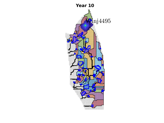
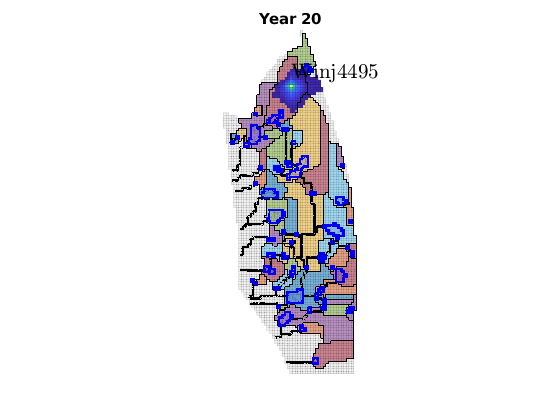
Simple example of pressure-limited injection for CO2 storage¶

Generated from pressureLimitedExample.m

This example uses the Bjarmeland formation, which is part of the Norwegian Petroleum Directorate’s Compiled CO2 Storage Atlas of the Norwegian Continental Shelf, found here: http://www.npd.no/en/Publications/Reports/Compiled-CO2-atlas/

% We use a fairly coarsened version of this formation dataset, to reduce
% the required time to run this example. Coarsening is controlled upon call
% to makeBjarmelandModel().

mrstModule add ad-core optimization
saveResults = false;

Set up simple example¶

The Bjarmeland model is set up with two wells, placed downstream from very large structural traps. Their initial rates are set based on the trapping capacity of these traps (using prior knowledge of trapping structure). However, in this example, we scale down the initial rates because it is not possible to operate at such large injection rates without comprimising the integrity of the caprock (i.e., the pressure limit becomes surpassed).

init_scale = 0.01; % scale down the total injected masses (kg)
qt = init_scale.*[3.7028e12; 2.6198e12];
[model, schedule, initState, seainfo, other] = makeBjarmelandModel( 'qt',qt );

% Initial simulation:
[init.wellSols, init.states] = simulateScheduleAD(initState, model, schedule, ...
                             'NonLinearSolver', NonLinearSolver('useRelaxation', true));
init.schedule = schedule;

Loading module libgeometry
Warning: Nan permeability values are being replaced with the average value.
Warning: Nan porosity values are being replaced with the average value.
Warning: Nan net-to-gross values are being replaced with the average value.
Loading module matlab_bgl
Loading module coarsegrid
Trap level 1: 13 traps identified
Trap level 2: 1 traps identified
...

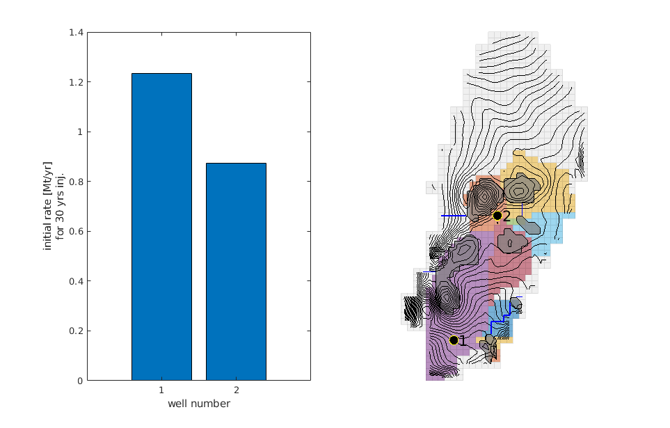
Set up¶

The cell pressure limit is set to be 90% of the overburden pressure, which is the weight of the fluid and solid layers lying on top of the formation we are injecting into. Cell pressure which surpasses this limit will be penalized by the objective function, using an optimization strategy in which the penalty factor is gradually ramped up as the iterations of the optimization scheme progress. Convergence to the optimal solution is reached once cell pressure surpasses the pressure limit by a tolerance of 2%. Leakage is also penalized by the objective function, and here we use a penalty factor of 5.

P_over = computeOverburdenPressure(model.G, model.rock, seainfo.seafloor_depth, model.fluid.rhoWS);
p_lim_fac   = 0.9;
P_limit     = P_over * p_lim_fac;
cP = [1e-9, 1e-8, 1e-7, 1e-6, 1e-5, 1e-4, 1e-3, 1e-2, 1e-1]; % pressure penalty factor
cL = 5; % leakage penalty factor
rate_lim_fac = 2; % max well controls are defined in terms of non-scaled qt

Evaluate initial objective (using lowest cP):¶

obj_funA = @(wellSols, states, schedule, varargin) ...
            leakPenalizerAtInfinity(model, wellSols, states, ...
                schedule, cL, other.surface_pressure, ...
                model.fluid.rhoWS, other.ta, varargin{:});
obj_funB = @(states, varargin) ...
            pressurePenalizer(model, states, schedule, cP(1), ...
                P_limit, varargin{:});

% Scale initial objective using obj_funA since obj_funB can be very large
init.obj_val_steps_A = cell2mat( obj_funA(init.wellSols, init.states, init.schedule) );
init.obj_val_steps_B = cell2mat( obj_funB(init.states) );
init.obj_val_steps = init.obj_val_steps_A - init.obj_val_steps_B;
init.obj_val_total = sum(init.obj_val_steps);
%obj_scaling = abs(init.obj_val_total);
obj_scaling = abs( sum(init.obj_val_steps_A) );

init0 = init; % keep the initial simulation results

Loading module ad-props
Loading module ad-blackoil
Total injected: 83192575.186177 (m3)
Total leaked (by infinity): 361786.536925 (m3)
Penalty: 5.000000
Score: 81383642.501555 (m3)

Surpassed Plimit by 0.000000 (percent) of Plimit.
...

More set up¶

We set how small and how high the well rates are allowed to be, which constrains our optimization problem within a “box”.

% Define limits and scaling based on initial simulation:
min_wvals       = sqrt(eps) * ones(numel(schedule.control(1).W), 1);
max_wvals       = rate_lim_fac * max( [schedule.control(1).W.val]' ./ init_scale ) ...
                    * ones(numel(schedule.control(1).W), 1);

Loop through pressure penalty factors until convergence reached within¶

tolerance of 2% of P_limit

sch = schedule;
for r = 1:numel(cP)
    cP_curr = cP(r);

    % Must re-define pressure penalizer with current penalty factor
    obj_funB = @(states, varargin) ...
                pressurePenalizer(model, states, sch, cP_curr, ...
                    P_limit, varargin{:});

    obj_fun = @(wellSols, states, schedule, varargin) ...
                cellSubtract(  obj_funA(wellSols, states, schedule, varargin{:}), ...
                    obj_funB(states, varargin{:})   );


    % Optimize injection rates
    % using the BFGS optimization algorithm. Passing in 'obj_scaling' means
    % an initial simulation will not be executed by optimizeRates. The
    % initial schedule is as per 'sch'.
    [optim, init, history] = optimizeControls(initState, model, sch, min_wvals, max_wvals, ...
                                'obj_fun',                      obj_fun, ...
                                'last_control_is_migration',    true, ...
                                'obj_scaling',                  obj_scaling, ...
                                'lineSearchMaxIt',              5, ...
                                'gradTol',                      1e-3, ...
                                'objChangeTol',                 1e-3);


    % Decide whether to ramp up cP or whether convergence reached
    [~, perc_of_Pover_reach] = ...
        findMaxPercentagePlimitReached( optim.states, P_limit, P_over );

    if (perc_of_Pover_reach/100 - p_lim_fac) > 0.02
        % use optimized rates as next iteration's initial rates
        sch = optim.schedule;
        % NB: init_scale won't reduce these rates
        % NB: max_wvals won't be in terms of these rates
    elseif r == numel(cP)
        warning('Convergence did not occur before or using last pressure penalty factor.')
    else
        % open system: if p < (plim + tolerance), optimal rates found
        break % exit cp(r) loop
    end

end

Solving timestep 01/80:           -> 1 Year
Solving timestep 02/80: 1 Year    -> 2 Years
Solving timestep 03/80: 2 Years   -> 3 Years
Solving timestep 04/80: 3 Years   -> 4 Years
Solving timestep 05/80: 4 Years   -> 5 Years
Solving timestep 06/80: 5 Years   -> 6 Years
Solving timestep 07/80: 6 Years   -> 7 Years
Solving timestep 08/80: 7 Years   -> 8 Years
...

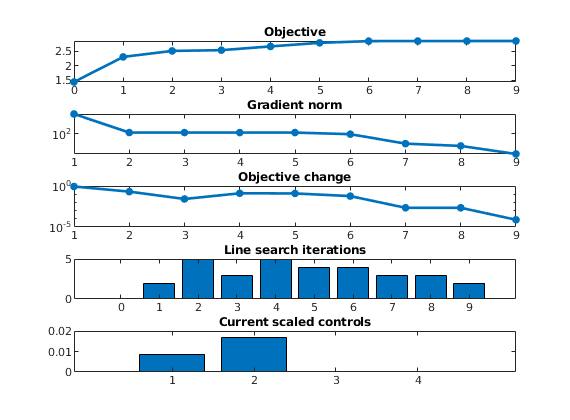
Saving¶

add variables to ‘other’, used for post-processing

other.fluid = model.fluid;
other.initState = initState;
other.leak_penalty = cL;
Gt = model.G;

if saveResults
    dirName = 'pressureLimitedExampleResults';
    mkdir(dirName);
    save(fullfile(dirName, 'Gt'),       'Gt');
    save(fullfile(dirName, 'optim'),    'optim');
    save(fullfile(dirName, 'init0'),    'init0');
    save(fullfile(dirName, 'init'),     'init');
    save(fullfile(dirName, 'history'),  'history');
    save(fullfile(dirName, 'other'),    'other'); % @@ fluid structure is quite large
end

Post-processing¶

The following figures will be generated: 1. well placement with trapping structure 2. initial co2 saturation 3. optimized co2 saturation 4. overburden pressure 5. max fraction of overburden pressure reached 6. initial vs optimized well rates 7. initial vs optimized trapping inventory (with forecast curves) 101: breakdown of forecast given initial rates 102: breakdown of forecast given optimized rates

close all
postProcessExample(Gt, init0, optim, other);

Total injected: 83192575.186177 (m3)
Total leaked (by infinity): 361786.536925 (m3)
Penalty: 5.000000
Score: 81383642.501555 (m3)

Total injected: 246976843.914029 (m3)
Total leaked (by infinity): 1736152.103265 (m3)
Penalty: 5.000000
...

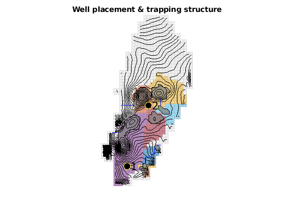
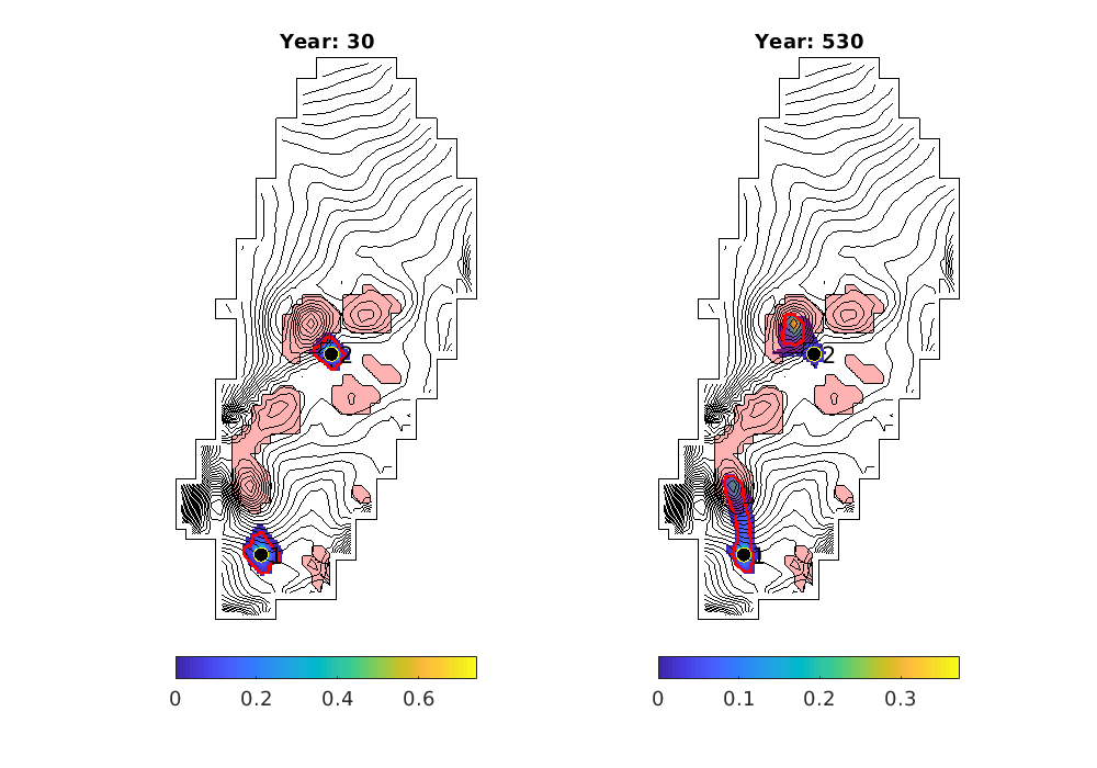
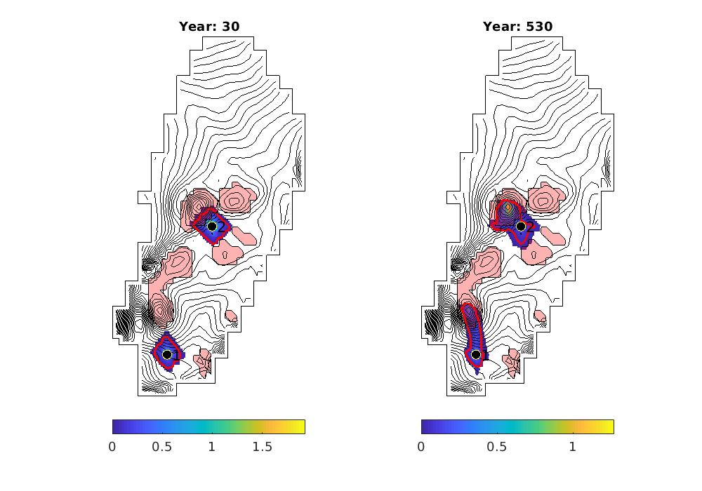
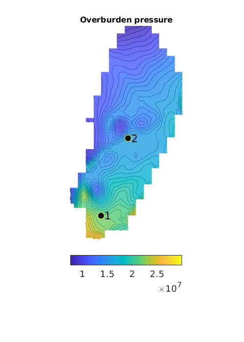
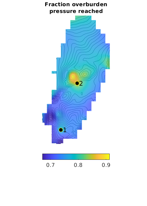
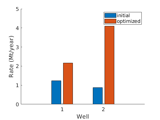
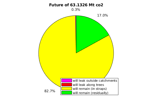
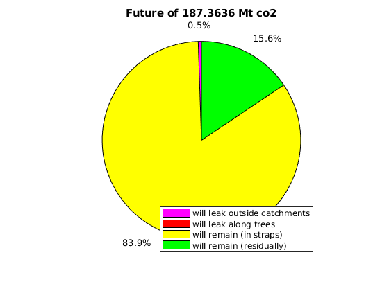
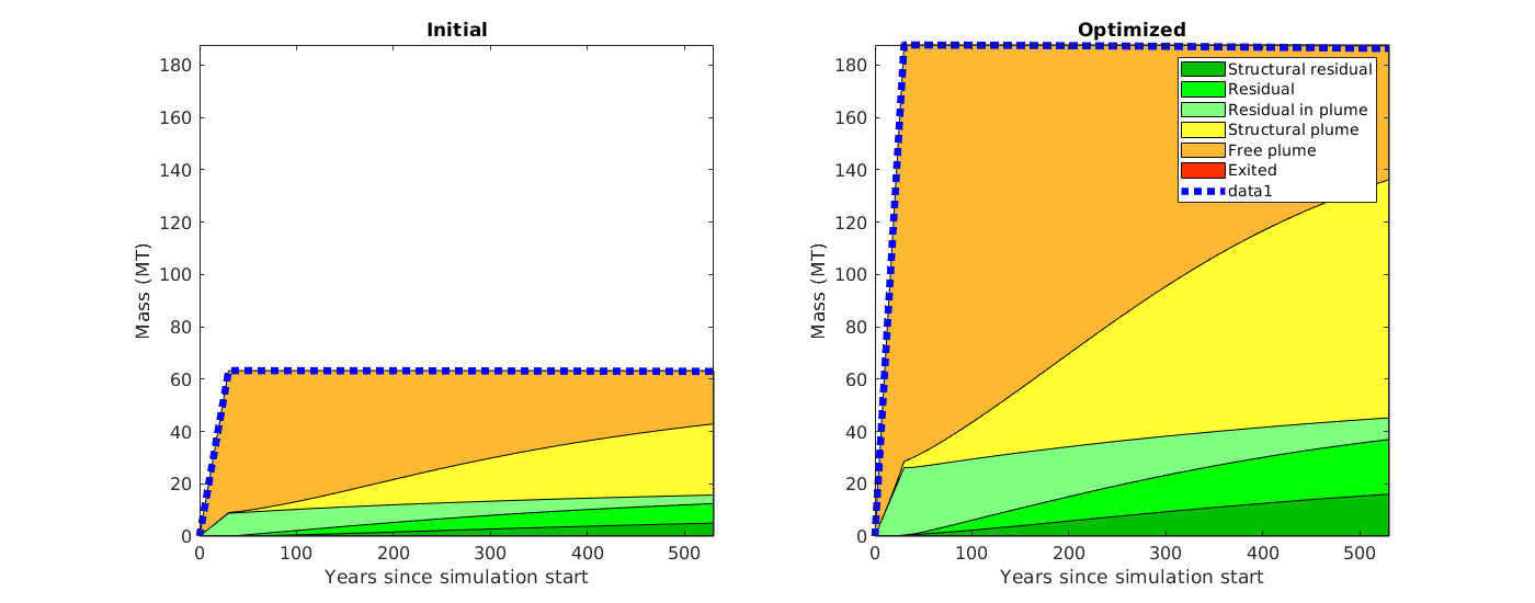
VE-incomp: Comparison of h and S-formulation¶

Generated from introExample.m

MRST-co2lab has two different types of vertical equilibrium solvers. What we for brevity will refer to as the VE-incomp solvers assume incompressible flow and are written much in the same way as the solvers in the incomp module. The VE-ad solvers rely on the AD-OO frame work implemented in ad-core/ad-blackoil, etc. This example will introduce you to the VE-incomp solvers. To this end, we consider a simple 1D example and compare the two different ways incompressible VE-models can be formulated:

The example also sets up a complete input deck (in Eclipse format) which can be used for simulation by traditional black-oil solvers like those implemented in the AD-OO framework.

mrstModule add co2lab incomp

Background¶

We start with the multiphase version of Darcy’s law:

$v_{\alpha}= - \frac{1}{\mu} K k_{r\alpha}(s_{\alpha}) (\nabla p_{\alpha} - \rho_{\alpha} \nabla z), \qquad \alpha=\{\mathrm{CO_2},\mathrm{water}\}.$

By integrating in the vertical direction and assuming vertical equlibrium with a sharp interface between the two fluids and constant permeability and porosity, we obtain the upscaled version of Darcy’s law

$V_{\alpha}= - \frac{1}{\mu} K k_{r\alpha}(1) h (\nabla_{\parallel} P_{\alpha}- \rho_{\alpha} \nabla_{\parallel} z), \qquad \alpha=\{\mathrm{CO_2},\mathrm{water}\}.$

If we now introduce

as the fractional height

of the CO2 column, Darcy’s law can be reformulated using

as variable

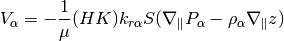
$V_{\alpha}= - \frac{1}{\mu} (HK) k_{r\alpha} S (\nabla_{\parallel} P_{\alpha}- \rho_{\alpha} \nabla_{\parallel} z)$

As usual the pressure equation from incompressible flow is obtaind by

$\nabla\cdot v = q, \qquad v=\sum_{\alpha} V_{\alpha},$

where

is the Darcy velocity (total velocity) and

is the total mobility, which depends on the water saturation

.

The transport equation (conservation of the CO2 phase) in its simplest form for the S-formulation

$\phi \frac{\partial S}{\partial t} + \nabla \cdot (f(S)(v + K \lambda_o (\nabla_{\parallel} (p_c + \rho z) )) = q_w$

and for the

formulation

$\phi \frac{\partial h}{\partial t} + \nabla \cdot (f(h) (v + K \lambda_o (\nabla_{\parallel} (p_c + \rho z) )) = q_w$

Notice, however, that the fractional flow functions

and the capillary pressure function

have a different interpretation than in a standard fractional flow model.

moduleCheck deckformat mimetic

Loading module deckformat
Loading module mimetic

Parameters for the simulation¶

gravity on
[nx,ny,nz] = deal(50, 1, 1);     % Cells in Cartsian grid
[Lx,Ly,H]  = deal(2000,1000,15); % Physical dimensions of reservoir
total_time = 100*year;           % Total simulation time
nsteps     = 200;                % Number of time steps in simulation
dt         = total_time/nsteps;  % Time step length
inj_time   = total_time/10;      % Injetection time
perm       = 100;                % Permeability in milli darcies
K          = perm*milli*darcy(); % Permeability in SI units
phi        = 0.1;                % Porosity
depth      = 1000;               % Initial depth
ipress     = 200;                % Initial pressure

Create input deck and convert to SI units¶

Create an input deck that can be used together with standard black-oil solvers. To this end, the 2D reservoir is described as a volumeric slice of a 3D reservoir.

deck = sinusDeck([nx ny nz], [Lx Ly H], nsteps, dt, -pi/180, depth, phi, ...
                 perm, (H*phi*Lx*Ly)*0.2*day/inj_time, ipress);
deck = convertDeckUnits(deck);

Instantiate grid and rock structures¶

Read the input deck to create a 3D grid, from which we can construct the top-surface grid used for the vertical equilibrium calculations

G = initEclipseGrid(deck);
G = computeGeometry(G);

Gts = topSurfaceGrid(G);
Gts.cells.H = H*ones(Gts.cells.num,1);
Gts.columns.dz = ones(numel(Gts.columns.cells),1)*H/nz;
Gts.columns.z = cumulativeHeight(Gts);

% get permeability
rock   = initEclipseRock(deck);
rock2d = averageRock(rock, Gts);

% Note that the top-surface grid is modified with an extra field that
% defines a function handle to how to calculate the gravity contribution.
% This is the part which is VE spesific.
Gts.grav_pressure

ans =

  function_handle with value:

    @(G,omega)gravPressureVE_s(G,omega)

Define boundary conditions, source terms, and fluid properties¶

Boundary conditions are no-flow and there are no source terms. Hence, these need not be specified explicitly, but we include them as a hook if the reader wants to extend the routine to more general cases.

[bc_s, bc_h]   = deal([]);
[src_s, src_h] = deal([]);
for i=1:numel(src_h)
    src_h.sat = nan;
    src_h.h = Gts.cells.H(src_s.cell);
end

% Extract fluid properties from input deck, but use different saturations.
mu = [deck.PROPS.PVDO{1}(1,3), deck.PROPS.PVTW(1,4)];
rho = deck.PROPS.DENSITY(1:2);
sr = 0.3;
sw = 0.3;

Define wells¶

We extract arbitrarily the first set of wells from the deck constructed for a general black-oil solver. Since the grid specified in the input deck is only one cell thick, the well indices calculated in 3D will also be correct for the VE simulation. However, we need to make two other modifications. First, if the well is specified as ‘resv’, we change the specification to rate. Likewise, we correct the definition of input value according to solver so that CO2 is injected correctly in each two-phase VE solver.

W_3D = processWells(G, rock, deck.SCHEDULE.control(1));
for i=1:numel(W_3D)
    if(strcmp(W_3D(i).type,'resv'))
        W_3D(i).type='rate';
    end
end
W_h = convertwellsVE(W_3D, G, Gts, rock2d,'ip_tpf');
W_s = convertwellsVE(W_3D, G, Gts, rock2d,'ip_tpf');
for i=1:numel(W_h)
    W_s(i).compi=[1 0];
    W_h(i).compi=nan;
    W_h(i).h = Gts.cells.H(W_h(i).cells);
end

Warning: Reference depth for well BHP in well 'I01' is set below well's top-most
reservoir connection
Warning: Reference depth for well BHP in well 'P01' is set below well's top-most
reservoir connection
Warning: Reference depth for well BHP in well 'I01' is set below well's top-most
reservoir connection
Warning: Reference depth for well BHP in well 'P01' is set below well's top-most
reservoir connection
...

Set up solver based on h-formulation¶

Create a cell array to hold helper variables and function handles for each solver.

problem = cell(2,1);
tmp.fluid = initVEFluidHForm(Gts, 'mu', mu, 'rho', rho, 'sr', sr,'sw', sw);
tmp.sol   = initResSol(Gts, 0);

% Set up wells, boundary conditions and source terms
[tmp.W, tmp.bc, tmp.src] = deal(W_h, bc_h, src_h);

% Define pressure and transport solvers with common interfaces. For the
% mimetic pressure solver, we need to precompute inner products
S = computeMimeticIPVE(Gts,rock2d,'Innerproduct','ip_tpf');
tmp.psolver = @(sol, fluid, W, bc, src) ...
   solveIncompFlowVE(sol, Gts, S, rock2d, fluid, 'wells', W, 'bc', bc, 'src', src);
tmp.tsolver = @(sol,fluid, dt, W, bc, src) ...
   explicitTransportVE(sol, Gts, dt, rock, fluid, 'computeDt', true, ...
   'intVert_poro', false,'intVert',false,'wells',W,'bc',bc, 'src', src);

% As this solver solves for the height of the CO2 plume, it is not
% neccessary to compute h from saturation values, but instead we have to
% compute the saturation from h
tmp.compute_h=false;
tmp.compute_sat=true;

% Miscellaneous
tmp.col  ='r-';
tmp.name = 'H formulation using explicit transport and mimetic discretization';

% Insert in cell array
problem{1} = tmp;
clear tmp

Set up solver based on S-formulation¶

The S-formulation uses standard solvers, except for the function handle ‘twophaseJacobian’ in the solution object, which here points to a slightly extended version of the original formulation of the Jacobi system (‘twophaseJacobian’) normally used in MRST

tmp.fluid = initSimpleVEFluid_s('mu', mu, 'rho', rho, ...
                                'height', Gts.cells.H, 'sr', [sr, sw]);
tmp.sol   = initResSolVE_s(Gts, 0, [1 0]);
tmp.sol.twophaseJacobian

% Set up wells, boundary conditions and source terms
[tmp.W, tmp.bc, tmp.src] = deal(W_s, bc_s, src_s);

% For the TPFA pressure solver, we need to calculate transmissibilities for
% the 2D top-surface grid. Depending on the definition of area and length
% in the top-surface grid this may or may not treat length along the
% surface.
T = computeTrans(Gts,rock2d);
T = T.*Gts.cells.H(gridCellNo(Gts));
tmp.psolver = @(sol,fluid, W, bc, src) ...
   incompTPFA(sol, Gts, T, fluid, 'wells', W, 'bc', bc, 'src', src);
tmp.tsolver = @(sol,fluid,dt,W,bc, src) ...
   implicitTransport(sol, Gts, dt, rock2d, fluid, 'wells', W, 'bc', bc, 'src', src);

% One needs to calculate h separatly since the solver does not
tmp.compute_h = true;
tmp.compute_sat = false;

% Miscellaneous
tmp.col = 'gs';
tmp.name = 'S formulation using implicit transport and two point flux';

% Insert in cell array
problem{2} = tmp;
clear tmp;

ans =

  function_handle with value:

    @twophaseJacobianWithVE_s

Initialize solution and variables¶

for kk=1:numel(problem)
    s0 = deck.SOLUTION.SOIL;
    h0 = deck.SOLUTION.SOIL.*Gts.cells.H;
    problem{kk}.sol.s = s0;
    problem{kk}.sol.h = h0;
    problem{kk}.sol.extSat = [s0, s0];
    problem{kk}.sol.h_max = h0;

    % Timers for pressure and transport solve
    problem{kk}.p_time=0;
    problem{kk}.t_time=0;
end

% Variables used for plotting
xc = Gts.cells.centroids(:,1);
zt = Gts.cells.z;
zb = Gts.cells.H+zt;
vol  = rock2d.poro.*Gts.cells.volumes.*Gts.cells.H;

Run the transport simulation.¶

fig1 = figure(1); p=get(fig1,'Position'); set(fig1,'Position', [p(1:2) 1020 420]);
fig2 = figure(2);

fprintf(1,' Free volumes [1e6 m^3]\n');
fprintf(1,'Time     H-form     S-form\n');
fprintf(1,'------------------------------\n');
fprintf(1,'%6.2f   %f   %f\n', 0.0, 0.0, 0.0);
t = 0;
while t < total_time
    set(0, 'CurrentFigure', fig1); clf
    set(0, 'CurrentFigure', fig2); clf
    for kk=1:numel(problem)
        tmp = problem{kk};

        if(t<inj_time)
           [W, bc, src] = deal(tmp.W, tmp.bc, tmp.src);
        else
           [W, bc, src] = deal([]);
        end

        % Solve the pressure
        timer = tic;
        tmp.sol = tmp.psolver(tmp.sol, tmp.fluid,  W, bc, src);
        tmp.p_time = tmp.p_time + toc(timer);

        % Using the computed fluxes, solve the transport
        timer = tic;
        if t>inj_time
           % uncomment to forcing zero total flow
           tmp.sol.flux(:) = 0;
        end
        tmp.sol = tmp.tsolver(tmp.sol,tmp.fluid,dt,W,bc, src);
        tmp.t_time =tmp.t_time + toc(timer);

        if tmp.compute_h
            % Compute h if this problem needs it
            [h, h_max]    = tmp.fluid.sat2height(tmp.sol);
            tmp.sol.h     = h;
            tmp.sol.h_max = h_max;

            % set the value s_max for convenience
            tmp.sol.s_max = tmp.sol.extSat(:,2);
        end
        if tmp.compute_sat
            % if the solver does not compute s and s_max, calculate them
            h     = tmp.sol.h;
            h_max = tmp.sol.h_max;
            tmp.sol.s =  (h*(1-sw) + (h_max - h)*sr)./Gts.cells.H;
            tmp.sol.s_max =  h_max*(1 - sw)./Gts.cells.H;
        end

        % Special type of plot if solving a 2D VE problem
        if Gts.cartDims(2)>1
            subplot(numel(problem),2,(2*(kk-1))+1)
            pcolor(X,Y,reshape(tmp.sol.h,Gts.cartDims))
            if kk==1, cxs=caxis(); else caxis(cxs); end;
            title(['Height ',num2str(kk)]);
            colorbar,shading interp

            subplot(numel(problem),2,(2*(kk-1))+2)
            pcolor(X,Y,reshape(tmp.sol.max_h,Gts.cartDims))
            caxis(cxs)
            title(['Max Height',num2str(kk)]);colorbar,shading interp

            problem{kk} = tmp;
            continue;
        end

        % Plot current and observed maximal values for h and S
        set(0, 'CurrentFigure', fig1);
        subplot(2,4,1), hold on
        plot(xc, tmp.sol.h, tmp.col); ylim([0 H])
        if kk==1, axh=axis(); else axis(axh); end
        title('Height'); xlabel('x'); ylabel('h');

        subplot(2,4,2), hold on
        plot(xc, tmp.sol.h_max, tmp.col); ylim([0 H])
        if kk==1, axh_max=axis(); else axis(axh_max);  end
        title('Max height'); xlabel('x'); ylabel('h_max') ;

        subplot(2,4,5), hold on
        plot(xc, tmp.sol.s(:,1), tmp.col); ylim([0 1])
        if kk==1; axs=axis(); else axis(axs); end
        title('Saturation'); xlabel('x'); ylabel('s')

        subplot(2,4,6), hold on
        plot(xc, tmp.sol.s_max(:,1), tmp.col); ylim([0 1]);
        if kk==1, axs_max=axis(); else axis(axs_max); end
        title('Max Saturation'); xlabel('x'); ylabel('s_max')

        set(0, 'CurrentFigure', fig1);
        subplot(2,4,[3 4 7 8]); set(gca,'YDir','reverse')
        hold on
        plot(xc,zt+tmp.sol.h, [tmp.col(1) '-'])
        plot(xc,zt+tmp.sol.h_max, [tmp.col(1), '--'])
        if kk==2
           patch(xc([1 1:end end]), [min(zt)-1; zt; min(zt)-1], .85*[1 1 1]);
           patch(xc([1 1:end end]), [max(zb)+1; zb; max(zb)+1], .85*[1 1 1]);
           legend('Free CO2, h', 'Max CO2, h', 'Free CO2, S', 'Max CO2, S', ...
                  'location', 'south');
           box on;axis tight; title('Surfaces'); xlabel('x'); ylabel('depth')
        end

        % Plot pressures.
        set(0, 'CurrentFigure', fig2); set(gca, 'YDir', 'reverse')
        hold on
        plot(xc, tmp.sol.pressure/barsa, tmp.col)
        if ~tmp.compute_sat
           % Also plot CO2 pressure: The default is to use the pressure of
           % the second phase pressure for the incompressible solvers
           plot(xc,(tmp.sol.pressure-tmp.fluid.pc(tmp.sol)),['-',tmp.col])
        else
           plot(xc,(tmp.sol.pressure-norm(gravity)*rho(1)*tmp.sol.h),['s',tmp.col])
        end
        xlabel('x'); ylabel('pressure')
        title('Comparing pressure for the different solvers')

        % Update solution object
        problem{kk} = tmp;
    end
    set(0, 'CurrentFigure', fig1); drawnow;
    set(0, 'CurrentFigure', fig2); drawnow;

    t=t+dt;

    % Print CO2 inventory
    fprintf(1,'%6.2f   %f   %f\n', t/year, ...
       sum(problem{1}.sol.s.*vol)/1e6, ...
       sum(problem{2}.sol.s.*vol)/1e6 );

end
fprintf(1,'-----------------------------------------\n\n');

Free volumes [1e6 m^3]
Time     H-form     S-form
------------------------------
  0.00   0.000000   0.000000
  0.50   0.030000   0.030000
  1.00   0.060000   0.060000
  1.50   0.090000   0.089999
  2.00   0.120000   0.119991
...

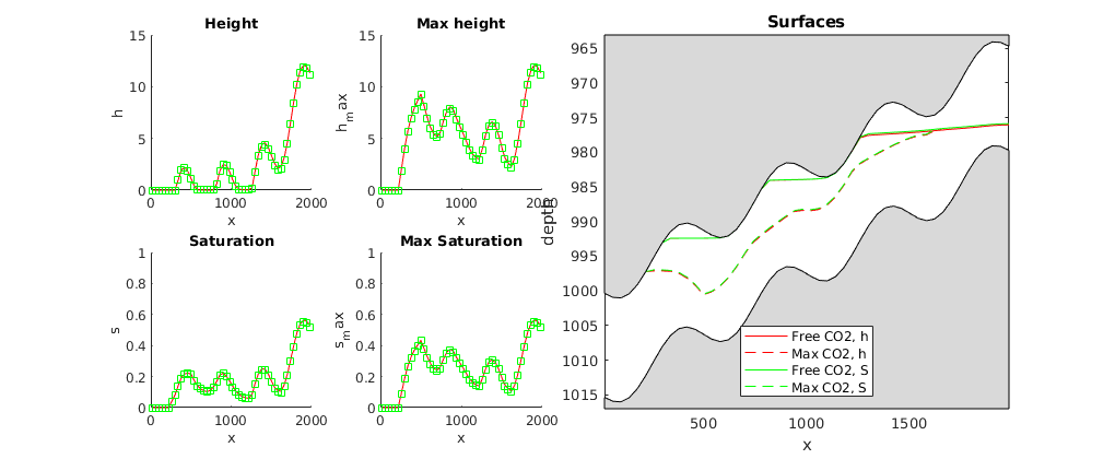
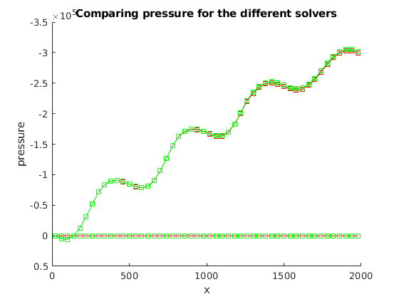
Output calculation time¶

for kk = 1:numel(problem)
   fprintf('Time used for solving with:\n\t%s\n',problem{kk}.name);
   fprintf('\tPressure time : %2.2d sec\n' ,problem{kk}.p_time)
   fprintf('\tTransport time : %2.2s sec\n',problem{kk}.t_time)
end

Time used for solving with:
      H formulation using explicit transport and mimetic discretization
      Pressure time : 7.15e-01 sec
      Transport time : 1.12e+00 sec
Time used for solving with:
      S formulation using implicit transport and two point flux
      Pressure time : 4.06e-01 sec
      Transport time : 7.46e+00 sec

Compare with analytical pressure¶

The state is almost stationary and we therefore add a comparison with pressures computed analytically. In the example, it is always only water at the bottom. For hydrostatic conditions, we can therefore find the pressure at the bottom relative to a given datum (here, we use the pressure at the top of the first column).

set(0, 'CurrentFigure', fig2); clf, hold on
set(gca, 'YDir', 'reverse')

p   = tmp.sol.pressure(1);
hh  = problem{1}.sol.h;
hs  = problem{2}.sol.h;
rwg = rho(2)*norm(gravity);
z   = Gts.cells.z;
H   = Gts.cells.H;

% Water pressure at the bottom
pwb = p + rwg*(z - z(1) + H(1));
plot(xc, pwb,'dk-')
text(xc(6),pwb(5), '\leftarrow Water pressure at bottom', ...
   'HorizontalAlignment', 'left')

% Water pressure extrapolated hydrostatic to the top of the reservoir
pwt = p + rwg*(z - z(1));
plot(xc, pwt, 'dk-')
text(xc(end-4), pwt(end-3), 'Water extrapolated to top \rightarrow', ...
   'HorizontalAlignment', 'right')

% water pressure at interface between CO2 and water
pwi = p + rwg*(z - z(1) + hh);
plot(xc, pwi,'dk-')
text(xc(10),pwi(7),'\uparrow Pressure at interface')

% CO2 pressure at the top surface
pco2 = p + rwg*(z+-z(1)+H(1)) - norm(gravity)*(rho(2)*(H - hs) + rho(1)*hs);
plot(xc, pco2, 'dr-');
text(xc(end-4), pco2(end-3),'Pressure at top \rightarrow', ...
   'HorizontalAlignment', 'right', 'Color', 'r')

% In this plot of the pressure at the end of simulation, we see that
%    - the mimetic method calculates the pressure at the interface between
%      CO2 and water
%    - the TPFA method with the given fluid calculates the extrapolated
%      water pressure at the top

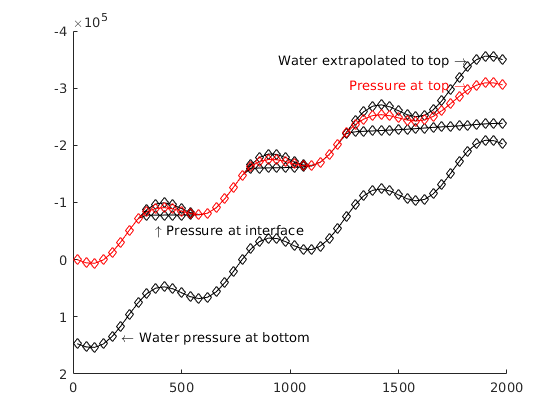
Vertical-Averaged Simulation of the Johansen Formation¶

Generated from runJohansenVE.m

The Johansen formation is a candidate site for large-scale CO2 storage offshore the south-west coast of Norway. In the following, we will use a simple vertically averaged model to simulate the early-stage migration of a CO2 plume injected from a single well positioned near the main fault in the formation. The formation is described by a geological model that has been developed based on available seismic and well data. A more thorough presentation of the geological model can be found in the script showJohansen.m

The data files necessary to run the example can be downloaded from the MatMoRA website.

mrstModule add co2lab mimetic

Display header¶

clc;
disp('================================================================');
disp('   Vertical averaging applied to the Johansen formation');
disp('================================================================');
disp('');

================================================================
   Vertical averaging applied to the Johansen formation
================================================================

Input data and construct grid models¶

We use a sector model in given in the Eclipse input format (GRDECL). The model has five vertical layers in the Johansen formation and five shale layers above and one below in the Dunhil and Amundsen formations. The shale layers are removed and we construct the 2D VE grid of the top surface, assuming that the major fault is sealing, and identify all outer boundaries that are open to flow. Store grid and rock structures to file to avoid time-consuming processing.

[G, rock, ~, Gt, rock2D, bcIxVE] = makeJohansenVEgrid();

-> Reading Johansen.mat

Set time and fluid parameters¶

gravity on
T          = 500*year();
stopInject = 100*year();
dT         = 2*year();
dTplot     = 1*dT;

% Fluid data at p = 300 bar
muw = 0.30860;  rhow = 975.86; sw    = 0.1;
muc = 0.056641; rhoc = 686.54; srco2 = 0.2;
kwm = [0.2142 0.85];

fluidVE = initVEFluidHForm(Gt, 'mu' , [muc muw] .* centi*poise, ...
                             'rho', [rhoc rhow] .* kilogram/meter^3, ...
                             'sr', srco2, 'sw', sw, 'kwm', kwm);

Set well and boundary conditions¶

We use one well placed in the center of the model, perforated in layer 6. Injection rate is 1.4e4 m^3/day of supercritical CO2. Hydrostatic boundary conditions are specified on all outer boundaries that are not in contact with the shales; the latter are assumed to be no-flow boundaries.

% Set well in 3D model
wellIx = [51, 51, 6, 6];
rate = 1.4e4*meter^3/day;
W = verticalWell([], G, rock, wellIx(1), wellIx(2), wellIx(3):wellIx(4),...
   'Type', 'rate', 'Val', rate, 'Radius', 0.1, 'comp_i', [1,0], ...
   'name', 'I', 'InnerProduct', 'ip_simple');

% Well and BC in 2D model
WVE = convertwellsVE(W, G, Gt, rock2D);

bcVE = addBC([], bcIxVE, 'pressure', Gt.faces.z(bcIxVE)*rhow*norm(gravity));
bcVE = rmfield(bcVE,'sat');
bcVE.h = zeros(size(bcVE.face));

Warning: Reference depth for well BHP in well 'I' is set below well's top-most
reservoir connection

Prepare simulations¶

Compute inner products and instantiate solution structure For the transport simulation, the default choice is to use a C-accelerated solver, but if this does not work, we use the standard solver from MRST.

SVE = computeMimeticIPVE(Gt, rock2D, 'Innerproduct','ip_simple');
preComp = initTransportVE(Gt, rock2D);
sol = initResSolVE(Gt, 0, 0);
sol.wellSol = initWellSol(W, 300*barsa());
sol.s = height2Sat(sol, Gt, fluidVE);
% select transport solver
try
   mtransportVE;
   cpp_accel = true;
catch me
   d = fileparts(mfilename('fullpath'));
   disp('mex-file for C++ acceleration not found');
   disp(['See ', fullfile(mrstPath('co2lab'),'ve','VEmex','README'),...
      ' for building instructions']);
   disp('Using matlab ve-transport');
   cpp_accel = false;
end

mex-file for C++ acceleration not found
See /home/francesca/mrstReleaseCleanRepo/mrst-bitbucket/mrst-co2lab/co2lab/ve/VEmex/README for building instructions
Using matlab ve-transport

Prepare plotting¶

We will make a composite plot that consists of several parts: a 3D plot of the plume, a pie chart of trapped versus free volumes, a plane view of the plume from above, and two cross-sections in the x/y directions through the well

opts = {'slice', wellIx, 'Saxis', [0 1-fluidVE.res_water], 'maxH', 100, ...
   'Wadd', 500, 'view', [-85 70], 'wireH', true, 'wireS', true};
plotPanelVE(G, Gt, W, sol, 0.0, zeros(1,4), opts{:});

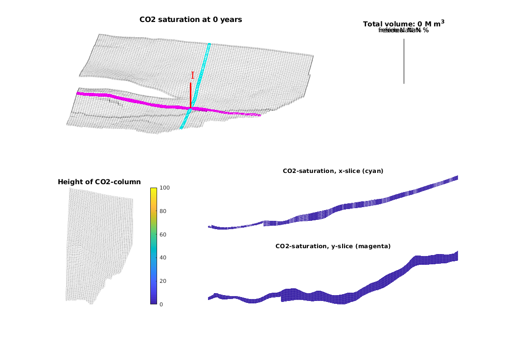
Main loop¶

Run the simulation using a sequential splitting with pressure and transport computed in separate steps. The transport solver is formulated with the height of the CO2 plume as the primary unknown and the relative height (or saturation) must therefore be reconstructed.

t = 0;
totVol = 0.0;
fprintf(1,'\nSimulating %d years on injection',convertTo(stopInject,year));
fprintf(1,' and %d years of migration\n', convertTo(T-stopInject,year));
fprintf(1,'Time: %4d years', convertTo(t,year));
tic;
while t<T
   % Advance solution: compute pressure and then transport
   sol = solveIncompFlowVE(sol, Gt, SVE, rock, fluidVE, ...
      'bc', bcVE, 'wells', WVE);

   if cpp_accel
        [sol.h, sol.h_max] = mtransportVE(sol, Gt, dT, rock, ...
                                fluidVE, 'bc', bcVE, 'wells', WVE, ...
                               'gravity', norm(gravity), 'verbose', false);
   else
      sol = explicitTransportVE(sol, Gt, dT, rock, fluidVE, ...
                                'bc', bcVE, 'wells', WVE, ...
                                'preComp', preComp);
   end

   % Reconstruct 'saturation' defined as s=h/H, where h is the height of
   % the CO2 plume and H is the total height of the formation
   sol.s = height2Sat(sol, Gt, fluidVE);
   assert( max(sol.s(:,1))<1+eps && min(sol.s(:,1))>-eps );
   t = t + dT;

   % Compute total injected, trapped and free volumes of CO2
   if ~isempty(WVE)
      totVol = totVol + WVE.val*dT;
   end
   vol = volumesVE(Gt, sol, rock2D, fluidVE);

   % Check if we are to stop injecting
   if t>= stopInject
      WVE  = []; bcVE = []; dT = 5*year(); dTplot = dT;
   end

   % Plotting
   fprintf(1,'\b\b\b\b\b\b\b\b\b\b%4d years', convertTo(t,year));
   if mod(t,dTplot)~= 0 && t<T,
      continue
   else
      plotPanelVE(G, Gt, W, sol, t, [vol totVol], opts{:});
      drawnow
   end
%    break
end
fprintf(1,'\n\n');

% delete C++ simulator
if cpp_accel, mtransportVE(); end
etime = toc;
disp(['Elapsed simulation time: ', num2str(etime), ' seconds.']);

Simulating 100 years on injection and 400 years of migration
Time:  500 years

Elapsed simulation time: 46.4583 seconds.

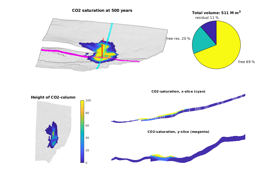
Vertical-Averaged Simulation: SLEIPNER¶

Generated from runSleipner.m

The Sleipner field in the North Sea was the world’s first commercial CO2 storage project. Every year since 1996, approximately one million tonnes of carbon dioxide has been captured from the natural gas production at Sleipner West using a conventional amine process and stored in the saline Utsira formation. The Utsira formation is a 200-250 meters thick massive sandstone that lies at a depth of 800-1000 metres below the seabed. In this example we simulate injection and migration of CO2 in the upper geological layer of Sleipner using the data provided in the paper:

The data set is avaliable online on: http://www.ieaghg.org/index.php?/2009112025/modelling-network.html

The data set provides injection rates for eleven years. We inject thirty years, assuming that the injection continues with a constant rate the last twenty years. We demonstrate the use of C/C++-accelerated MATLAB, using the functions

The last mentioned function requires that you have built the solver in the src/VEmex directory.

mrstModule add co2lab mimetic

Display header¶

clc
disp('================================================================');
disp('   Vertical averaging applied to the Sleipner model');
disp('   using C++ accelleration in the transport solver');
disp('================================================================');
disp(' ');

================================================================
   Vertical averaging applied to the Sleipner model
   using C++ accelleration in the transport solver
================================================================

Construct stratigraphic, petrophysical, and VE models¶

The 3D model consists of a grid (G) and petrophysical parameters (rock). The VE model consists of a top-surface grid (Gt), petrophysical data (rock2D), and indices to the boundarcy cells where we will supply pressure boundary conditions. Called with a true flag, the routine will use C-accelerated MATLAB routines to process the data input and compute geometry. Once the models are created, they are stored in a data file for faster access at a later time.

[G, Gt, rock, rock2D, bcIxVE] = makeSleipnerVEmodel('usemex',true, ...
                                                    'assign_coords',false);

-> Reading Sleipner.mat
    Data set has not yet been constructed.
 -> Reading data from: /home/francesca/mrstReleaseCleanRepo/mrst-bitbucket/mrst-core/examples/data/Sleipner
 -> Processing grid
 -> Constructing top-surface grid
 -> Writing Sleipner.mat

Set time and fluid parameters¶

Fluid data are taken from paper SPE 134891

gravity on
T          = 250*year();
stopInject = 30*year();
dT         = 1*year();
dTplot     = dT;
fluidVE    = initVEFluidHForm(Gt, 'mu' , [6e-2*milli 8e-4]*Pascal*second, ...
                              'rho', [760 1200] .* kilogram/meter^3, ...
                              'sr', 0.21, 'sw', 0.11, 'kwm', [0.75 0.54]);

Set well and boundary conditions¶

The well is placed near the actual injection site. The injection rates are taken from the beforementioned paper. Hydrostatic boundary conditions are specified on all outer boundaries.

disp(' -> Setting well and boundary conditions');

% Set well in 3D model
wellIx = [36 78 7];
rates  = [2.91e4; 5.92e4; 6.35e4; 8.0e4; 1.09e5; ...
         1.5e5; 2.03e5; 2.69e5; 3.47e05; 4.37e5; 5.4e5]*meter^3/year;
W      = verticalWell([], G, rock, wellIx(1), wellIx(2), ...
                      wellIx(3), 'Type', 'rate', 'Val', rates(1), ...
                      'Radius', 0.1, 'comp_i', [1,0], 'name', 'I');

% Well in 2D model
WVE = convertwellsVE(W, G, Gt, rock2D);

% BC in 2D model
bcVE = addBC([], bcIxVE, 'pressure', ...
            Gt.faces.z(bcIxVE)*fluidVE.rho(2)*norm(gravity));
bcVE = rmfield(bcVE,'sat');
bcVE.h = zeros(size(bcVE.face));

-> Setting well and boundary conditions
Warning: Reference depth for well BHP in well 'I' is set below well's top-most
reservoir connection

Prepare simulations¶

Compute inner products and instantiate solution structure

disp(' -> Initialising solvers');
SVE = computeMimeticIPVE(Gt, rock2D, 'Innerproduct','ip_simple');
preComp = initTransportVE(Gt, rock2D);
sol = initResSolVE(Gt, 0, 0);
sol.wellSol = initWellSol(W, 300*barsa());
sol.s = height2Sat(sol, Gt, fluidVE);

% Find trapping structure in grid. Used for calculation of trapped volumes
ts=findTrappingStructure(Gt);

% Select transport solver
% Use C++ acceleration if it exists - NB: requires the VEmex module
% Notice that the two solvers determine the time steps differently and
% may therefore give slightly different answers.
try
   mtransportVE;
   cpp_accel = true;
catch me
   disp('mex-file for C++ acceleration not found');
   disp(['See ', fullfile(mrstPath('co2lab'),'ve','VEmex','README'), ...
      ' for building instructions']);
   disp('Using matlab VE-transport');
   cpp_accel = false;
end

-> Initialising solvers
Trap level 1: 196 traps identified
Trap level 2: 34 traps identified
Trap level 3: 2 traps identified
Trap level 4: 1 traps identified
mex-file for C++ acceleration not found
See /home/francesca/mrstReleaseCleanRepo/mrst-bitbucket/mrst-co2lab/co2lab/ve/VEmex/README for building instructions
Using matlab VE-transport

Prepare plotting¶

We will make a composite plot that consists of several parts: a 3D plot of the plume, a pie chart of trapped versus free volume, a plane view of the plume from above, and two cross-sections in the x/y directions through the well

opts = {'slice', wellIx, 'Saxis', [0 1-fluidVE.res_water], ...
   'maxH', 5, 'Wadd', 10, 'view', [130 50]};
plotPanelVE(G, Gt, W, sol, 0.0, zeros(1,6), opts{:});

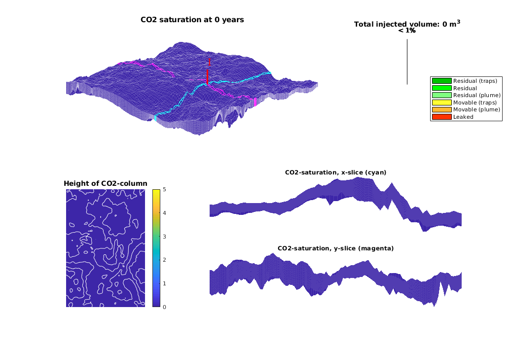
Main loop¶

Run the simulation using a sequential splitting with pressure and transport computed in separate steps. The transport solver is formulated with the height of the CO2 plume as the primary unknown and the relative height (or saturation) must therefore be reconstructed.

t = 0;
totVol = 0.0;
fprintf(1,'\nSimulating %d years of injection', convertTo(stopInject,year));
fprintf(1,' and %d years of migration\n', convertTo(T-stopInject,year));
fprintf(1,'Time: %4d years', convertTo(t,year));

w = WVE;
tic
while t<T
   % Advance solution: compute pressure and then transport
   sol = solveIncompFlowVE(sol, Gt, SVE, rock, fluidVE, ...
      'bc', bcVE, 'wells', w);

   if cpp_accel
      [sol.h, sol.h_max] = mtransportVE(sol, Gt, dT, rock, ...
                                          fluidVE, 'bc', bcVE, 'wells', w, ...
                                          'gravity', norm(gravity));
   else
      sol = explicitTransportVE(sol, Gt, dT, rock, fluidVE, ...
                               'bc', bcVE, 'wells', w, 'preComp', preComp, ...
                               'intVert', false);
   end

   % Reconstruct 'saturation' defined as s=h/H, where h is the height of
   % the CO2 plume and H is the total height of the formation
   sol.s = height2Sat(sol, Gt, fluidVE);
   assert( max(sol.s(:,1))<1+eps && min(sol.s(:,1))>-eps );
   t = t + dT;

   % Add the volume injected during last time step to the total volume
   % and compute trapped and free volumes
   if ~isempty(w)
      totVol = totVol + w.val*dT;
   end
   vol = volumesVE(Gt, sol, rock2D, fluidVE, ts);

   % Check if we are to stop injecting or change injection rate
   if t>= stopInject
      w  = []; dT = 5*year(); dTplot = dT;
   else
      ind = min(floor(t/year)+1, numel(rates));
      w.val = rates(ind);
   end

   % Plotting
   fprintf(1,'\b\b\b\b\b\b\b\b\b\b%4d years', convertTo(t,year));
   if mod(t,dTplot)~= 0 && t<T,
      continue
   else
      plotPanelVE(G, Gt, W, sol, t, [vol totVol], opts{:});
      drawnow
   end
end
fprintf(1,'\n\n');
% delete C++ simulator
if cpp_accel, mtransportVE; end
etime = toc;
disp(['Elapsed simulation time: ', num2str(etime), ' seconds.']);

Simulating 30 years of injection and 220 years of migration
Time:  250 years

Elapsed simulation time: 253.5172 seconds.

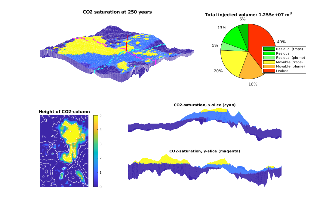
Show the structural trap¶

After the simulation has completed, we are interested in seeing how the location of the CO2 plume after a long migration time corresponds to the trapping estimates produced by trapAnalysis. This is done by finding the trap index of the well injection cell and then plotting the trap along with the final CO2 plume.

% Generate traps and find the trap corresponding to the well cells
res = trapAnalysis(Gt, false);
trap = res.trap_regions([WVE.cells]);

% Plot the areas with any significant CO2 height along with the trap in red
clf;
plotCellData(Gt, sol.h, sol.h > 0.01)
plotGrid(Gt, res.traps == trap, 'FaceColor', 'red', 'EdgeColor', 'w')
h = plotGrid(Gt, 'FaceColor', 'None', 'EdgeAlpha', .1);

legend({'CO2 Plume', 'Trap'})
axis tight off
view(-20, 75)
title('End of simulation CO2 compared to algorithmically determined trap')

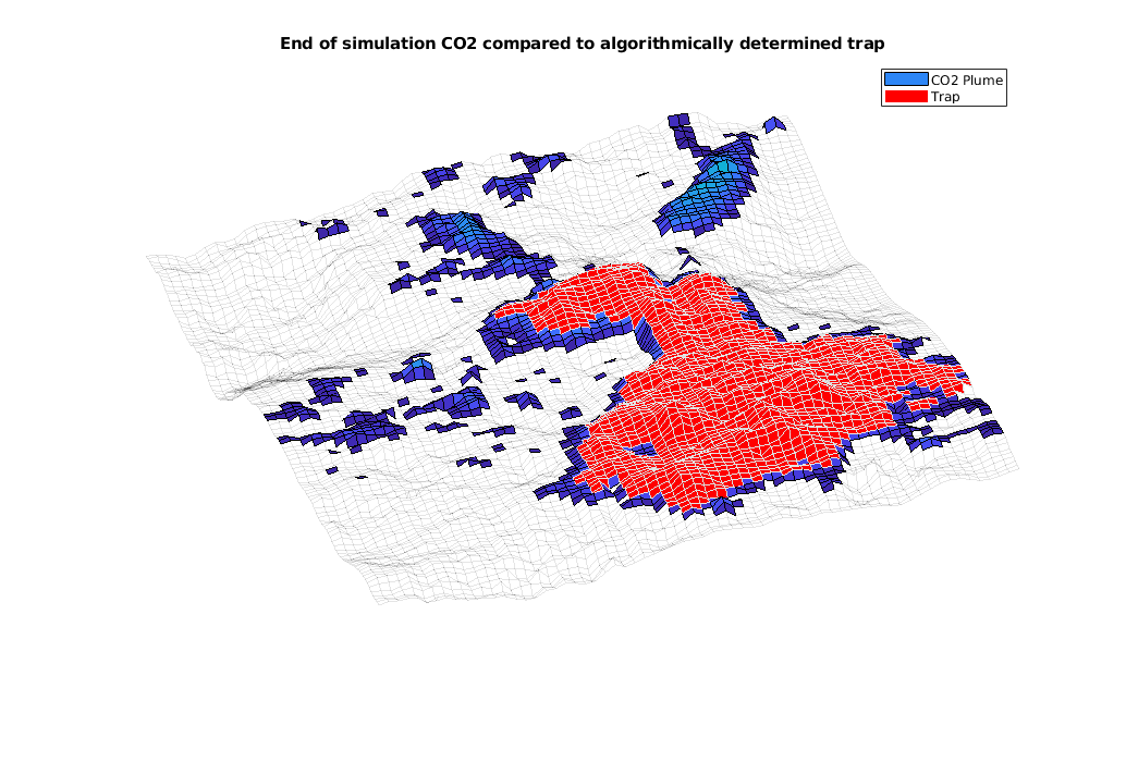
VE-incomp: C-accelerated simulation of sloping aquifer¶

Generated from runSlopingAquifer.m

The incompressible VE solvers also have an accelerated back-end solver written in C. This example demonstrates this solver for a synthetic model of a sloping aquifer. The topography of the top surface and the geological layers in the model are generated by combining the membrane function (MATLAB logo) and a sinusoidal surface with random perturbations. CO2 is injected in the aquifer for a period of 30 years. Thereafter we simulate the migration of the CO2 in a post-injection period of 720 years.

mrstModule add co2lab

Write header¶

clear, clc;
disp('================================================================');
disp('   Vertical averaging applied to a synthetic sloping aquifer');
disp('   using C++ accelleration in the transport solver');
disp('================================================================');
disp(' ');

================================================================
   Vertical averaging applied to a synthetic sloping aquifer
   using C++ accelleration in the transport solver
================================================================

Construct stratigraphic and petrophysical model¶

We construct a slightly sloping aquifer with a wavy top surface that allows for structural trapping

[G, Gt, rock, rock2D, bcIxVE] = makeSlopingAquifer();

-> Reading SlopingAquifer.mat

Set time and fluid parameters¶

Inject CO2 for 30 years and study subsequent migration until 750 years after injection started. The fluid data are chosen so that they are resonable at p = 300 bar

gravity on
T          = 500*year();
stopInject = 30*year();
dT         = 2*year();
dTplot     = 2*dT;
fluidVE    = initVEFluidHForm(Gt, 'mu' , [0.056641 0.30860] .* centi*poise, ...
                         'rho', [686.54 975.86] .* kilogram/meter^3, ...
                         'sr', 0.2, 'sw', 0.1, 'kwm', [0.2142 0.85]);

Set well and boundary conditions¶

We use one well placed down the flank of the model, perforated in the bottom layer. Injection rate is 1.4e3 m^3/day of supercritical CO2. Hydrostatic boundary conditions are specified on all outer boundaries.

% Set well in 3D model
wellIx = [G.cartDims(1:2)/5, G.cartDims([3 3])];
rate   = 2.8e3*meter^3/day;
W      = verticalWell([], G, rock, wellIx(1), wellIx(2), ...
                      wellIx(3):wellIx(4), 'Type', 'rate', 'Val', rate, ...
                      'Radius', 0.1, 'comp_i', [1,0], 'name', 'I', ...
                      'InnerProduct', 'ip_simple');

% Well and BC in 2D model
WVE = convertwellsVE(W, G, Gt, rock2D);

bcVE     = addBC([], bcIxVE, 'pressure', ...
                 Gt.faces.z(bcIxVE)*fluidVE.rho(2)*norm(gravity));
bcVE     = rmfield(bcVE,'sat');
bcVE.h   = zeros(size(bcVE.face));

Warning: Reference depth for well BHP in well 'I' is set below well's top-most
reservoir connection

Prepare simulations¶

Compute inner products and instantiate solution structure

SVE = computeMimeticIPVE(Gt, rock2D, 'Innerproduct','ip_simple');
preComp = initTransportVE(Gt, rock2D);
sol = initResSolVE(Gt, 0, 0);
sol.wellSol = initWellSol(W, 300*barsa());
sol.s = height2Sat(sol, Gt, fluidVE);

% Use C++ acceleration for the transport calculation
% NB: requires that the VEmex module has been compiled
try
   mtransportVE();
   cpp_accel = true;
catch me
   d = fileparts(mfilename('fullpath'));
   disp('mex-file for C++ acceleration not found');
   disp(['See ', fullfile(mrstPath('co2lab'),'ve','VEmex','README'), ...
      ' for building instructions']);
   disp('Using matlab ve-transport');
   cpp_accel = false;
end
moduleCheck('mimetic');

% Find trapping structure in grid. Used for calculation of trapped volumes
ts=findTrappingStructure(Gt);

mex-file for C++ acceleration not found
See /home/francesca/mrstReleaseCleanRepo/mrst-bitbucket/mrst-co2lab/co2lab/ve/VEmex/README for building instructions
Using matlab ve-transport
Loading module mimetic
Trap level 1: 90 traps identified
Trap level 2: 13 traps identified
Trap level 3: 2 traps identified

Prepare plotting¶

We will make a composite plot that consists of several parts, a 3D plot of the plume, a pie chart of trapped versus free volume, a plane view of the plume from above, and two cross-sections in the x/y directions through the well

opts = {'slice', wellIx,  'maxH', 15, 'Saxis', [0 1-fluidVE.res_water], ...
   'view', [-7, 25], 'Wadd', 100};
plotPanelVE(G, Gt, W, sol, 0.0, zeros(1,6), opts{:});

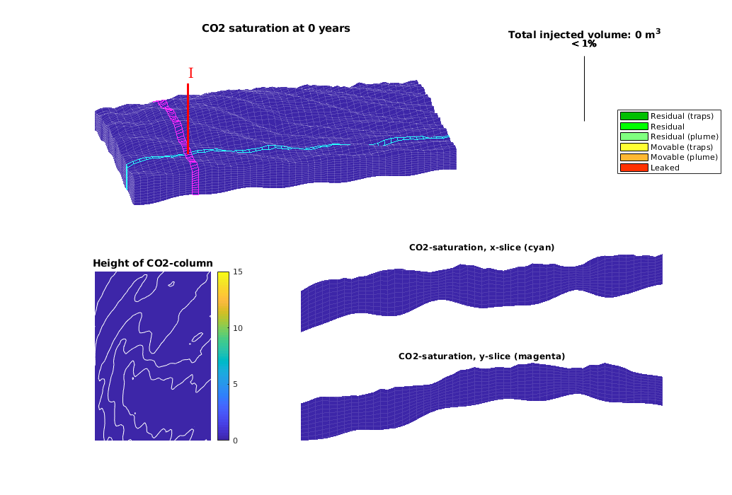
Main loop¶

Run the simulation using a sequential splitting with pressure and transport computed in separate steps. The transport solver is formulated with the height of the CO2 plume as the primary unknown and the relative height (or saturation) must therefore be reconstructed.

t = 0;
totVol = 0;
fprintf(1,'\nSimulating %d years of injection',convertTo(stopInject,year));
fprintf(1,' and %d years of migration\n', convertTo(T-stopInject,year));
fprintf(1,'Time: %4d years', convertTo(t,year));

sol_mex   = sol;
while t<T
   % Advance solution: compute pressure and then transport
   sol = solveIncompFlowVE(  sol, Gt, SVE, rock, fluidVE, ...
                             'bc', bcVE, 'wells', WVE);

   if cpp_accel
      [sol.h, sol.h_max] = mtransportVE(sol, Gt, dT, rock, ...
                                fluidVE, 'bc', bcVE, 'wells', WVE, ...
                               'gravity', norm(gravity), 'verbose', false);
   else
      sol = explicitTransportVE(sol, Gt, dT, rock, fluidVE, ...
                             'bc', bcVE, 'wells', WVE, 'preComp', preComp);
   end

   % Reconstruct 'saturation' defined as s=h/H, where h is the height of
   % the CO2 plume and H is the total height of the formation
   sol.s = height2Sat(sol, Gt, fluidVE);
   assert( max(sol.s(:,1))<1+eps && min(sol.s(:,1))>-eps );
   t = t + dT;

   % Compute total injected, trapped and free volumes of CO2
   if ~isempty(WVE)
      totVol = totVol + WVE.val*dT;
   end
   vol = volumesVE(Gt, sol, rock2D, fluidVE, ts);

   % Check if we are to stop injecting
   if t>= stopInject
      WVE  = []; dT = 10*year(); dTplot = dT;
   end

   % Plotting
   fprintf(1,'\b\b\b\b\b\b\b\b\b\b%4d years', convertTo(t,year));
   if mod(t,dTplot)~= 0 && (t<T),
      continue
   else
      plotPanelVE(G, Gt, W, sol, t, [vol totVol], opts{:});
      drawnow
   end

end
fprintf(1,'\n\n');
% delete C++ simulator
if cpp_accel, mtransportVE(); end

Simulating 30 years of injection and 470 years of migration
Time:  500 years

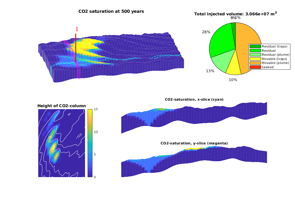
VE-incomp: C-Acceleration on Large Model¶

Generated from runSlopingAquiferBig.m

In this example we consider a synthetic sloping aquifier that has a significant variation in the top-surface morphology. We demonstrate the use of C/C++-accelerated MATLAB, using the function mtransportVE to replace explicitTransportVE. Using mtransportVE requires that you have built the solver in the VEmex directory. In addition, the routine makeIGEMSmodel that sets up the data model may use the following C-accelerated MATLAB routines

mrstModule add co2lab

Write header¶

clc;
disp('================================================================');
disp('   Vertical averaging applied to a large model');
disp('   using C++ accelleration in the transport solver');
disp('================================================================');
disp(' ');

================================================================
   Vertical averaging applied to a large model
   using C++ accelleration in the transport solver
================================================================

Construct stratigraphic, petrophysical, and VE models¶

The 3D model consists of a grid (G) and petrophysical parameters (rock). The VE model consists of a top-surface grid (Gt), petrophysical data (rock2D), and indices to the boundarcy cells where we will supply pressure boundary conditions. Called with a true flag, the routine will use C-accelerated MATLAB routines to process the data input and compute geometry. Once the models are created, they are stored in a data file for faster access at a later time.

[G, Gt, rock, rock2D, bcIxVE] = makeSlopingAquiferBig(true);

-> Reading slopingAquiferBig.mat

Set time and fluid parameters¶

Inject CO2 for 150 years and study subsequent migration until 750 years after injection started. The fluid data are chosen so that they are resonable at p = 300 bar

gravity on
T          = 750*year();
stopInject = 150*year();
dT         = 2*year();
dTplot     = 2*dT;
fluidVE    = initVEFluidHForm(Gt, 'mu' , [0.056641 0.30860] .* centi*poise, ...
                         'rho', [686.54 975.86] .* kilogram/meter^3, ...
                        'sr', 0.2, 'sw', 0.1, 'kwm', [0.2142 0.85]);

Set well and boundary conditions¶

We use one well placed down the flank of the model, perforated in the bottom layer. Injection rate is 2.8e4 m^3/day of supercritical CO2. Hydrostatic boundary conditions are specified on all outer boundaries.

disp(' -> Setting well and boundary conditions');

% Set well in 3D model
wellIx = [G.cartDims(1:2)/5, G.cartDims([3 3])];
rate   = 2.8e4*meter^3/day;
W      = verticalWell([], G, rock, wellIx(1), wellIx(2), ...
                      wellIx(3):wellIx(4), 'Type', 'rate', 'Val', rate, ...
                      'Radius', 0.1, 'comp_i', [1,0], 'name', 'I', ...
                      'InnerProduct', 'ip_simple');

% Well in 2D model
WVE = convertwellsVE(W, G, Gt, rock2D);

% BC in 2D model
bcVE   = addBC([], bcIxVE, 'pressure', ...
            Gt.faces.z(bcIxVE)*fluidVE.rho(2)*norm(gravity));
bcVE   = rmfield(bcVE,'sat');
bcVE.h = zeros(size(bcVE.face));

-> Setting well and boundary conditions
Warning: Reference depth for well BHP in well 'I' is set below well's top-most
reservoir connection

Prepare simulations¶

Compute inner products and instantiate solution structure

disp(' -> Initialising solvers');
SVE = computeMimeticIPVE(Gt, rock2D, 'Innerproduct','ip_simple');
preComp = initTransportVE(Gt, rock2D);
sol = initResSolVE(Gt, 0, 0);
sol.wellSol = initWellSol(W, 300*barsa());
sol.s = height2Sat(sol, Gt, fluidVE);

% Select transport solver
% Use C++ acceleration if it exists - NB: requires the VEmex module
% Notice that the two solvers determine the time steps differently and
% may therefore give slightly different answers.
try
   mtransportVE();
   cpp_accel = true;
catch me
   d = fileparts(mfilename('fullpath'));
   disp('mex-file for C++ acceleration not found');
   disp(['See ', fullfile(mrstPath('co2lab'),'ve','VEmex','README'), ...
      ' for building instructions']);
   disp('Using matlab ve-transport');
   cpp_accel = false;
end
mrstModule add mimetic

% Find trapping structure in grid. Used for calculation of trapped volumes
ts=findTrappingStructure(Gt);

-> Initialising solvers
mex-file for C++ acceleration not found
See /home/francesca/mrstReleaseCleanRepo/mrst-bitbucket/mrst-co2lab/co2lab/ve/VEmex/README for building instructions
Using matlab ve-transport
Trap level 1: 643 traps identified
Trap level 2: 104 traps identified
Trap level 3: 17 traps identified
Trap level 4: 4 traps identified
...

Prepare plotting¶

We will make a composite plot that consists of several parts: a 3D plot of the plume, a pie chart of trapped versus free volume, a plane view of the plume from above, and two cross-sections in the x/y directions through the well

opts = {'slice', wellIx, 'Saxis', [0 1-fluidVE.res_water], ...
   'maxH', 200, 'Wadd', 1000};
plotPanelVE(G, Gt, W, sol, 0.0, zeros(1,6), opts{:});

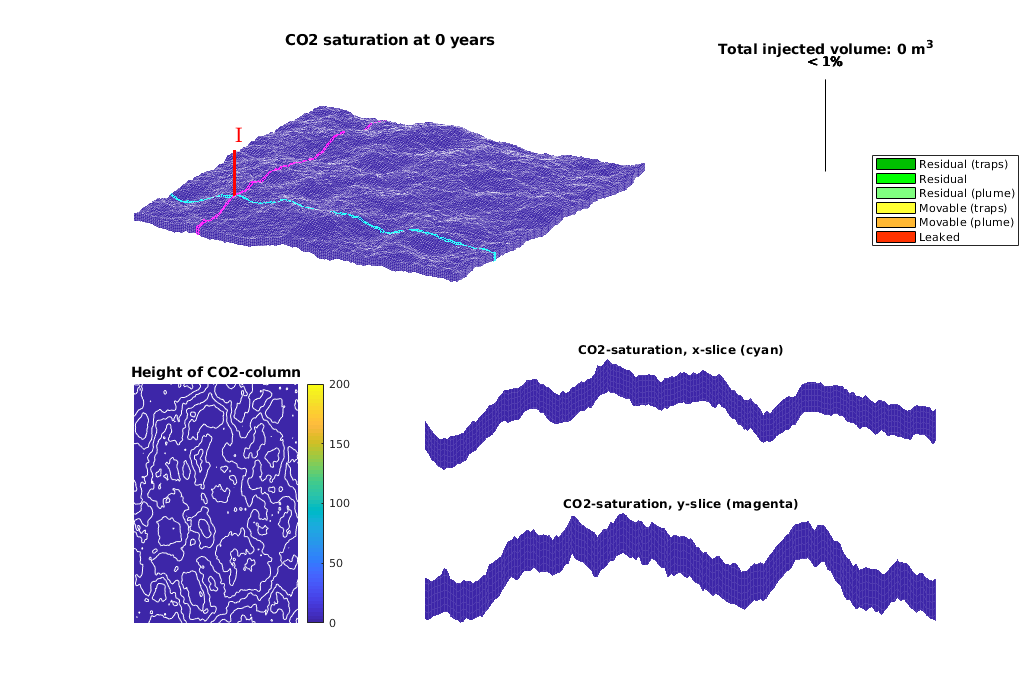
Main loop¶

Run the simulation using a sequential splitting with pressure and transport computed in separate steps. The transport solver is formulated with the height of the CO2 plume as the primary unknown and the relative height (or saturation) must therefore be reconstructed.

t = 0;
totVol = 0.0;
fprintf(1,'\nSimulating %d years of injection', convertTo(stopInject,year));
fprintf(1,' and %d years of migration\n', convertTo(T-stopInject,year));
fprintf(1,'Time: %4d years', convertTo(t,year));
tic
while t<T
   % Advance solution: compute pressure and then transport
   sol = solveIncompFlowVE(sol, Gt, SVE, rock, fluidVE, ...
      'bc', bcVE, 'wells', WVE);

   if cpp_accel
      [sol.h, sol.h_max] = mtransportVE(sol, Gt, dT, rock, ...
                                          fluidVE, 'bc', bcVE, 'wells', WVE, ...
                                          'gravity', norm(gravity));
   else
      sol = explicitTransportVE(sol, Gt, dT, rock, fluidVE, ...
                               'bc', bcVE, 'wells', WVE,    ...
                               'preComp', preComp,          ...
                               'intVert', false);
   end

   % Reconstruct 'saturation' defined as s=h/H, where h is the height of
   % the CO2 plume and H is the total height of the formation
   sol.s = height2Sat(sol, Gt, fluidVE);
   assert( max(sol.s(:,1))<1+eps && min(sol.s(:,1))>-eps );
   t = t + dT;

   % Compute total injected, trapped and free volumes of CO2
   if ~isempty(WVE)
      totVol = totVol + WVE.val*dT;
   end
   vol = volumesVE(Gt, sol, rock2D, fluidVE, ts);

   % Check if we are to stop injecting. If so, increase the time step.
   if t>= stopInject
      WVE  = []; dT = 10*year(); dTplot = dT;
   end

   % Plotting
   fprintf(1,'\b\b\b\b\b\b\b\b\b\b%4d years', convertTo(t,year));
   if mod(t,dTplot)~= 0 && t<T,
      continue
   else
      plotPanelVE(G, Gt, W, sol, t, [vol totVol], opts{:});
      drawnow
   end
end
fprintf(1,'\n\n');

% delete C++ simulator
if cpp_accel, mtransportVE(); end
etime = toc;
disp(['Elapsed simulation time: ', num2str(etime), ' seconds.']);

Simulating 150 years of injection and 600 years of migration
Time:  750 years

Elapsed simulation time: 228.7223 seconds.

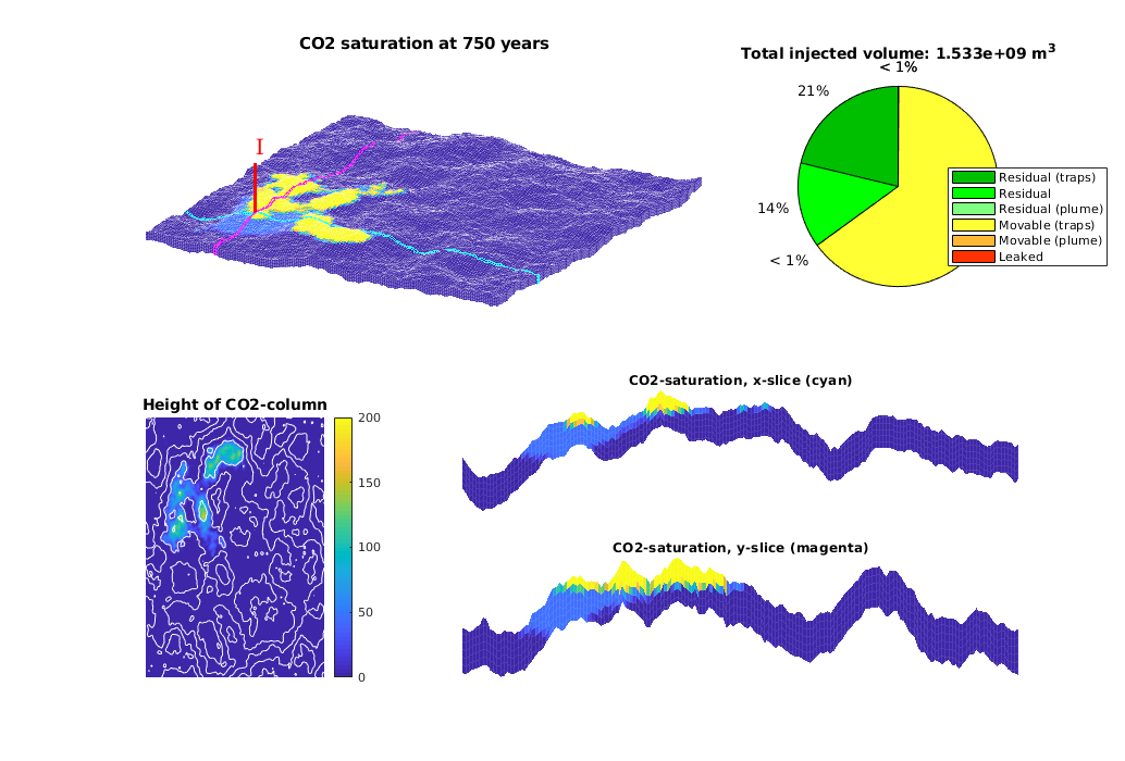
Simulate long term migration on the Utsira formation¶

Generated from runUtsira.m

This example demonstrates simulation of long-term migration of CO2 in the Utsira formation using incompressible flow and Dirichlet pressure boundary conditions. CO2 is injected in the cell nearest to the Sleipner field where CO2 injection is ongoing.

mrstModule add co2lab incomp

Set up fluid properties and hydrostatic pressure¶

We define approximate hydrostatic pressure for a set of z values to use as initial values:

$P = P_0 + rho_{water}\cdot \delta h g_z$

At the same time, we define the physical properties of CO2 and water at our reference pressure. We also define a coarsening of the full Utsira grid. The full grid contains a fairly large number of cells, so we coarse by a factor 3. This can be changed to a higher or lower number depending on the available processing power and the patience of the user.

muw = 0.30860;  rhow = 975.86; sw    = 0.1;
muc = 0.056641; rhoc = 686.54; srco2 = 0.2;
kwm = [0.2142 0.85];

mu  = [muc  muw ] .* centi*poise;
rho = [rhoc rhow] .* kilogram/meter^3;

% Define reservoar top
topPos = 300*meter;
topPressure = 300*barsa;

% Turn on gravity
gravity on;
grav = gravity();

% Pressure function
pressure = @(z) topPressure + rho(2)*(z - topPos)*grav(3);

% Default viewing angle
v = [-80, 80];

% Coarsening factor
nc = 3;

Set up injection parameters¶

We inject a yearly amount of 1 Mt/year (which is approximately the same as the current injection at Sleipner) for a period of 100 years, followed by 4900 years of migration. During injection the timesteps are smaller than during migration.

T_tot = 5000*year;
T_inj =  100*year;

N = 20;
dT_inj  = T_inj / N;  % short time steps during injection
dT_long = dT_inj*5;   % longer steps during migration

% ~ 1Mt annual injection
rate = 1e9*kilogram/(year*rhoc*kilogram*meter^3);

% Approximate position of the Sleipner field
sleipnerPos = [438514, 6472100];

Set up a grid corresponding to the Utsira formation¶

The Sleipner field has a history of CO2 injection. It is embedded in the Utsira formation. We will demonstrate how the larger formation grids can be used to simulate long term migration.

[grids, info, petrodata] = getAtlasGrid('Utsirafm', 'nz', 5, 'coarsening', nc);

% Store heightmap data for contour plots
info = info(cellfun(@(x) strcmpi(x.variant, 'top'), info));
info = info{1};

G = processGRDECL(grids{1});

% Depending on the coarsening factor, occasionally very small subsets of
% cells may become disconnected. We guard against this by taking only the
% first grid returned by processGRDECL,  which is guaranteed by
% processGRDECL to be the one with the most cells.
G = G(1);
try
    % Try accelerated geometry calculations.
    G = mcomputeGeometry(G);
catch ex
    % Fall back to pure MATLAB code.
    G = computeGeometry(G);
end

[Gt, G] = topSurfaceGrid(G);

Plot grid along with top surface¶

We downshift the full grid to plot it alongside with the top surface. We also add a simple light to show the surface variation in height, which highlights regions where structural trapping is possible. To show the relation to the original dataset, we plot contour lines on the original height data. Note that as the final grid is the intersection between the provided height and thickness datasets, some contour lines do not correspond to any part of the grid.

figure;
Gplot = G;
Gplot.nodes.coords(:,3) = Gplot.nodes.coords(:,3) + 100;
plotCellData(Gt, Gt.cells.H, 'EdgeColor','none')
plotGrid(Gplot, 'edgea', .1)
light
lighting phong
view(v);
legend({'Top surface', 'Original grid (downshifted)'}, 'Location', 'North')
contourAtlas(info, 15, 1, 'k')
axis tight off

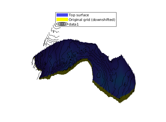
Set up rock properties and compute transmissibilities¶

We use the averaged values for porosity and permeability as given in the Atlas tables. Since cellwise data is not present, we assume to averaged values to be valid everywhere.

pd = petrodata{1};
rock.poro = repmat(pd.avgporo, G.cells.num, 1);
rock.perm = repmat(pd.avgperm, G.cells.num, 1);
rock2D    = averageRock(rock, Gt);
T = computeTrans(Gt, rock2D);
T = T.*Gt.cells.H(gridCellNo(Gt));

Set up fluid¶

fluid = initSimpleVEFluid_s('mu' , mu , 'rho', rho, ...
                            'height'  , Gt.cells.H,...
                            'sr', [srco2, sw],'kwm',kwm);

Set up well and boundary conditions¶

This example is using an incompressible model for both rock and fluid. If we assume no-flow on the boundary, this will result in zero flow from a single injection well. However, this can be compensated if we use the physical understanding of the problem to set appropriate boundary conditions: The Utsira formation is enormous compared to the volume of the injected CO2. Thus, it is impossible that the injection will change the composition of the formation significantly. We therefore assume that the boundary conditions can be set equal to hydrostatic pressure to drive flow.

% Find the cell nearest to the Sleipner field
si = findEnclosingCell(Gt, sleipnerPos);

% Add an injector well for the CO2
W = addWell([], G, rock, si,...
   'Type', 'rate', 'Val', rate, 'comp_i', [1,0], ...
   'name', 'Sleipner field', 'InnerProduct', 'ip_tpf');

% Add pressure boundary
bnd = boundaryFaces(Gt);
bc = addBC([], bnd, 'pressure', pressure(Gt.faces.z(bnd)), 'sat', [0 1]);

% Convert to 2D wells
W2D = convertwellsVE(W, G, Gt, rock2D,'ip_tpf');

Warning: Reference depth for well BHP in well 'Sleipner field' is set below
well's top-most reservoir connection

Set up initial reservoir conditions¶

The initial pressure is set to hydrostatic pressure. Setup and plot.

sol = initResSolVE_s(Gt, pressure(Gt.cells.z), 0);
sol.wellSol = initWellSol(W2D, 0);

clf;
plotCellData(Gt, sol.pressure, 'EdgeColor','none');
view(v); axis tight off; colorbar

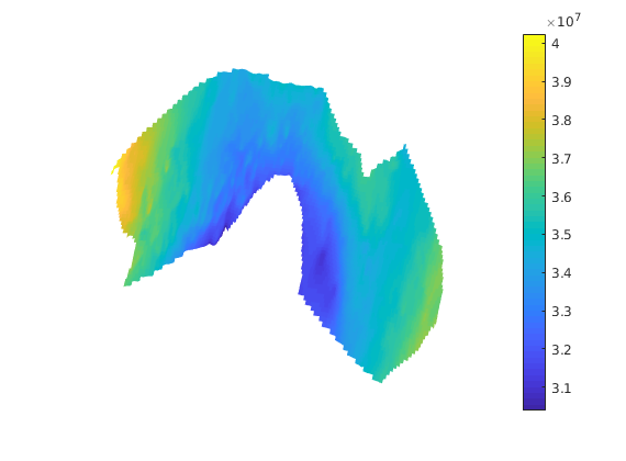
Run the simulation¶

Solve for all timesteps, and plot the results at each timestep.

t = 0;
dT = dT_inj;
tt = ' (Injecting)';
while t < T_tot;
    if t >= T_inj
        W2D = [];
        dT  = dT_long;
        tt  = ' (Migrating )';
    end
    sol = incompTPFA(sol, Gt, T,       fluid, 'wells', W2D, 'bc', bc);
    sol = implicitTransport(sol, Gt, dT, rock2D, fluid, 'wells', W2D, 'bc', bc, 'Verbose', true);
    t = t + dT;

    % Plotting
    [s, h] = normalizeValuesVE(Gt, sol, fluid);

    % Plot the whole formation
    subplot(2,1,1)
    cla
    plotCellData(G, s, 'edgec', 'k', 'edgea', .1, 'edgec', [.6 .6 .6]);
    plotWell(G, W); caxis([0 .9]);
    contourAtlas(info, 10, 1, 'k')
    title([formatTimeRange(t) tt])
    axis tight off
    view(v);

    % Plot the area around the Sleipner formation
    subplot(2,1,2)
    cla
    plotCellData(G, s, s > 1e-3);
    contourAtlas(info,25, 1, 'k')
    plotGrid(G, 'facec', 'none', 'edgec', [.6 .6 .6], 'edgea', .1)
    axis([4.2e5 4.6e5 6.45e6 6.5e6]), caxis([0 .9]);
    view(v);

    drawnow
end

implicitTransport:
----------------------------------------------------------------------
Time interval (s)     iter  relax   residual          rate
----------------------------------------------------------------------
 [0.0e+00, 1.6e+08]:   1    1.00    3.03200e-03              NaN
 [0.0e+00, 1.6e+08]:   2    1.00    2.16256e-05             1.60
 [0.0e+00, 1.6e+08]:   3    1.00    1.03633e-09             2.01
...

co2lab: Numerical CO2 laboratory¶

Examples¶

Grid Models from the CO2 Storage Atlas¶

Example: Utsira formation¶

Full 3D visualization of all grids in North Sea¶

Basic capacity estimates for the CO2 atlas data (North Sea)¶

CO2 Storage Atlas: the Norwegian North Sea¶

Read data¶

Description of raw data¶

Show the data directly: Utsira formation¶

Visualize all the formations¶

Redo the visualization in 3D with higher resolution¶

Johansen formation: the effect of coarsening on trapping¶

Plot a subset of the formation with different degree of coarsening¶

The effect of coarsening on trapping analysis¶

Trapping example¶

Make grid and rock data¶

Construct top surface grid¶

Geometric analysis of caprock (spill-point analysis)¶

Show connection between traps and spill paths¶

Compute the total trapping capacity¶

Plot leaf nodes¶

Plot accumulation areas using interactive viewer¶

Optimal injection points¶

Extract a subset of the Utsira formation for analysis¶

Compute trapping analysis and find the sorted injection trees¶

Find the ideal injection spot for each trap region¶

Alternative visualization¶

Top-Surface Grids¶

A simple 3D example: removing unconnected cells¶

Construct top-surface grid¶

Inspect the data structure: planar 2D grid¶

Numbering of cells in top-surface and 3D grid¶

Geometry information¶

Miscellaneous¶

Interactive spill point analysis of top surface grids¶

Explore a synthetic grid¶

The Johansen formation¶

Grid from the IGEMS¶

Effects of scales structures on trapping capacity¶

Load data and create grids¶

Trap analysis¶

Estimate the unresolved local oscillations per area¶

Extrapolate this estimate to the whole Utsira formation¶

Get another estimate by removing global trends¶

Find new trapping volume¶

Extrapolate this estimate to the whole Utsira formation¶

Compare trap of local variations to global variations¶

IGEMS Data Set¶

Read and prepare grid structure¶

First study: geometric analyisis of caprock (spill point analysis)¶

Inspect the Hugin West Formation¶

Show the whole formation with trapping structure¶

Extract a subset¶

Node-based traps¶

Cell-based traps¶

Trapping on Johansen grids¶

Load NPD data: sector model¶

Load NPD data: full-field model¶

Load atlas data¶

Plot the three data sets¶

Interactive trapping: atlas grid¶

Interactive trapping: NPD sector grid¶

Interactive trapping: NPD full-field grid¶

Brine Production Example¶

Set-up model and perform initial simulation¶

Define some parameters¶

Evaluate initial objective (using lowest cP):¶

Define min and max well control values (used to set up box limits)¶

Loop through pressure penalty factors until convergence reached within¶

Saving¶

VE simulation in a standard black-oil solver¶

Parameters for the simulation¶

Create input deck and construct grid¶

Initialize data structures¶

Show simulation grid¶

Prepare simulation model, schedule and initial state¶

Run the schedule setup in the file¶

Plot results¶

Examples to demonstrate forecast of CO2 leakage and its application¶

`co2lab`: Numerical CO₂ laboratory¶