nwm: Near Wellbore Modelling

class HorWellRegion(G, well, regionIndices, varargin)

Class for horizontal well (HW) region in volume of interest (VOI) grid which generates the geometrical information of VOI grid and constructs the radial HW grid

HorWellRegion(G, well, regionIndices, varargin)

The HW grid is built inside the Cartesian region of VOI grid. And the logical indices of HW region are specified.

1 ymin ymax ny

—– —– —– —– —– —– —–

| | | | | | | 1 —– —– —– —– —– —– —–

| * | * | * | * | * | | zmin —– —– —– —– —– —– —–

| * | * | * | * | * | | —– —– —– —– —– —– —–

| * | * | * | * | * | | zmax —– —– —– —– —– —– —–

| | | | | | | nz —– —– —– —– —– —– —–

• = HW region

Remarks: 1 < ymin < ymax < ny (GV.children.cartDims(2))

1 < zmin < zmax < nz (GV.layers.num)

regionIndices: [ymin, ymax, zmin, zmax]

IDOfFourVertices(hw)

Get the indices of four vertices in boundary nodes

ReConstructToRadialGrid(hw, radPara)

Reconstruct VOI grid in HW region to layered radial grid. Two types of grid lines are provided: ‘pureCircular’ : The radial grid lines are pure circular ‘gradual’ : The radial grid lines vary from the circular

line to the rectangular line of a specified box gradually

Parameters:

• GV – The layered VOI grid, built by ‘VolumeOfInterest.ReConstructGrid’
• radPara –

  Parameters for generating the radial grid The type ‘pureCircular’ requires following fields:

  ’maxRadius’: Max radius of the radial grid ‘nRadCells’: Number of radial cells

  The type ‘gradual’ requires following fields:

  ’boxRatio’ : Size ratio of the rectangular box

  to the outer boundary, 2x1 double, [yRatio, zRatio]

  ’nRadCells’: Number of radial cells, 2x1 double,

  [inbox, outbox]

  ’pDMult’ : Multiplier of pD of the outer-most

  angular line to PD of wellbore line, the larger the pDMult is, the outer-most line is closer to the box

  ’offCenter’: Whether the well is off-center in

  the radial grid

Returns:

GW – Layered radial HW grid

allInfoOfRegion(hw, varargin)

Get all information of the region, consisting of cells, layer-faces, nodes of layer-faces, boundary nodes, indices of vertices.

assignCartDimsOfVOIGrid(hw)

Assign Cartesian dimensions of VOI grid

assignRegionIndices(hw)

Assign the region indices

bdyNodesOfRegion(hw, varargin)

Get boundary nodes of HW region in VOI grid

cartCellsOfVOIGrid(hw, varargin)

Get cells of VOI grid in Cartesian region

cellsOfRegion(hw, varargin)

Get cells of HW region in VOI grid

checkRegionIndices(hw)

Check whether the region indices exceed the Cartesian reigon dimension of the VOI grid

facesOfRegion(hw, c, n, varargin)

Get layer-faces of HW region in VOI grid

getNodesSingleSurface(hw, varargin)

Get nodes of HW region in VOI grid on single surface

nodesOfRegion(hw, varargin)

Get nodes of layer-faces of HW region in VOI grid

plotRegionCells(hw, packed)

Plot cells inside the HW region

plotRegionLayerFaces(hw, packed)

Plot layer-faces of the HW region

showWellRegionInVOIGrid(hw, varargin)

Show the well region in the VOI grid

GVOI = None

Layered unstructured VOI grid

regionIndices = None

Logical indices of HW region in VOI grid

well = None

Structure of well information

class MultiSegWellNWM(subGrids, deck, well, varargin)

Derived class for generating necessary data structures passed to the mrst AD simulators for the hybrid grid of near-wellbore model coupling with the multi-segment well model

buildWellboreGrid(msw)

Build grid for the void space inside wellbore

generateNodes(msw)

Generate node definitions from the wellbore grid for multi-segment well

generateSegments(msw)

Generate segment definitions from the wellbore grid for multi-segment well

getSimSchedule(msw, model, varargin)

Get the multi-segment well simulation schedule from deck and node/segment definitions

plotSegments(msw, nodes, segs, S)

Plot the nodes and reservoir cells assoicated with segment S

setupSimModel(nwm, rock, T_all, N_all)

Setup simulation model passed to ad-blackoil simulator for the global grid (the multi-segment well model now only supports the ‘ThreePhaseBlackOilModel’) rock: Rock of the global grid T_all: Full transmissibility N_all: Neighborship of all connections

wellboreGrid = None

1D ‘wellbore grid’ in the void wellbore space which

class NearWellboreModel(subGrids, deck, well, varargin)

Class for generating necessary data structures passed to the mrst AD simulators for the hybrid grid of near-wellbore model

assembleTransNeighbors(nwm, T, nnc)

Assemble transmissibility and neighborship for the simulation model

assignInputSubGrdTypes(nwm, varargin)

Assign types of input subgrids

assignInputSubGrds(nwm, varargin)

Assign subgrids from input

assignSubGrdTypes(nwm, varargin)

Assign types of updated subgrids

assignSubGrds(nwm, varargin)

Assign updated subgrids from the global grid

assignSubRocks(nwm, rock)

Assign rocks from the global rock for updated subgrids

cellMapFromInputSubGrdsToGloGrd(nwm)

Cell map from input subgrids to global grid

cellMapFromSubGrdsToGloGrd(nwm)

Cell map from updated subgrids (after-remove cells) to global grid

checkCellMaps(nwm)

Check the cell maps

checkFaceMaps(nwm)

Check the face maps

checkIntxnRelation(nwm, intXn)

Check the intersection relation by comparing the face areas

computeCPGHalfTrans(nwm, rock)

Flow | Permeability | Anisotropy |

approximation | coordinate | |

|---------------------------------------------| | Linear | Local | Yes | ———————————————–

computeHWGrdHalfTrans(nwm, rock)

Flow | Permeability | Anisotropy |

approximation | coordinate | |

|---------------------------------------------| | Radial | Global | Yes | ———————————————–

computeIntxnRelation(nwm)

Compute intersection relations between subgrids

computeVOIGrdHalfTrans(nwm, rock)

Flow | Permeability | Anisotropy |

approximation | coordinate | |

|---------------------------------------------| | Linear | Global | No | ———————————————–

faceMapFromInputSubGrdsToGloGrd(nwm)

Face map from input subgrids to global grid

faceMapFromSubGrdsToGloGrd(nwm)

Face map from updated subgrids (after-remove cells) to global grid

generateNonNeighborConn(nwm, intXn, rock, T)

Generate the non-neighbor connections (NNCs) intXn: Boundary intersection relations rock: Rock of global grid T: Fully transmissibility of global grid

getCPGRockFromDeck(nwm)

Get the rock of input CPG from input deck

getCPGSimSchedule(nwm, model)

Get the simulation schedule for input CPG from deck

getGlobalRock(nwm, rocks)

Get the rock for the global grid rocks = {rockC, rockV, rockW} ————————————————————- | Rock | Grid | Source | Permeability | Anisotropy | | | | | coordinate | | |-----------------------------------------------------------| | rockC | Input | Input deck | Local | Yes | | | GC | | | | |-----------------------------------------------------------| | rockV | Input | Interpolation | Global | Yes | | | GV | of rockC | | | |-----------------------------------------------------------| | rockW | Input | User-defined | Global | No | | | GW | | | | ————————————————————-

getGrdEclFromDeck(nwm)

Get ECLIPSE grid structure from deck

getInitState(nwm, model)

Get initial state by equilibrium initialization

getPhaseFromDeck(nwm)

Get phase components from input deck

getRadTransFactors(nwm)

Get the radial half transmissibility factors for the HW grid Get the factors of the 2D surface grids first

getSimSchedule(nwm, model, varargin)

Get the simulation schedule for the global grid from the production/injection control data in deck

getTransGloGrid(nwm, rock)

Compute the transmissibility for the global grid rock: rock of the global grid The transmissibility consists of: Transmissibility of updated [CPG, VOI grid, and HW grid]

getVOIRocksByInterp(nwm, varargin)

Get the rock of input VOI grid by interpolation of CPG rock Optional:

‘InterpMethod’, same with opitions in ‘griddata’: ‘linear’ (default) | ‘nearest’ | ‘natural’ | ‘cubic’ | ‘v4’

getWellCellPara(nwm, model)

Get parameters for well cells of the HW wc: well cell indices wf: well face indices WI: well indices of well cells

getWellCells(nwm)

Get well cell indices

matchingIntxnRelation(nwm, grdInd)

Compute intersection relations of matching faces on the layered boundaries of input subgrids gridInd: Indices of the subgrids involving in the computation

[i-1, i], i <= number of subgrids

nncOfMatchingBoundaries(nwm, intXn, rock, T)

Generate non-neighbor connections (NNCs) arised from the matching boundaries intXn: Boundary intersection relations rock: Rock of global grid T: Fully transmissibility of global grid

nncOfNonMatchingBoundaries(nwm, intXn, rock, T)

Generate non-neighbor connections (NNCs) arised from the non-matching boundaries intXn: Boundary intersection relations rock: Rock of global grid T: Fully transmissibility of global grid

nonMatchingIntxnRelation(nwm, grdInd, bdyLoc)

Compute intersection relations of non-matching faces on the boundaries of input subgrids gridInd: Indices of the subgrids involving in the computation

[i-1, i], i <= number of subgrids

bdyLoc: The location of boundaries

‘top’ | ‘bot’ for CPG and VOI grid ‘heel’ | ‘toe’ for VOI grid and HW grid

packedCPGSimData(nwm)

Obtain all necessary simulation data structures of the CPG CPG

packedSimData(nwm, rockW, varargin)

Obtain all necessary simulation data structures of the hybrid grid in near-wellbore model Global grid

plotMatchingIntxnRelation(nwm, intXn, f1)

Plot the intersection relations of matching face f1

plotNonMatchingIntxnRelation(nwm, intXn, f1)

Plot the intersection relations of non-matching face f1

setupCPGSimModel(nwm)

Setup simulation model passed to ad-blackoil simulator for the input CPG grid

setupFluid(nwm)

Initialize AD fluid from input deck

setupSimModel(nwm, rock, T_all, N_all)

Setup simulation model passed to ad-blackoil simulator for the global grid rock: Rock of global grid T_all: Full transmissibility N_all: Neighborship of all connections

validateGlobalGrid(nwm, varargin)

Validate the global hybrid grid by subgrids Get updated subgrids (cells in VOI and HW region are removed)

fluid = None

AD-solver fluid from ECLIPSE-style input deck

gloGrid = None

The global hybrid grid

inputDeck = None

ECLIPSE-style input deck of CPG

subGrids = None

Subgrids {Corner-point grid (CPG), VOI grid, HW grid}

well = None

Structure of well information

class VolumeOfInterest(G, well, pbdy, nextra, varargin)

Class for volume of interest (VOI) in the Corner-point grid (CPG) or Cartesian grid which generates the geometrical information of CPG or Cartesian grid in VOI and constructs the unstructured VOI grid.

PeacemanWellCells(volume, varargin)

Find well cells of Peaceman’s well model, require ‘wellpaths’ module

ReConstructToUnstructuredGrid(volume, WR, layerRf, varargin)

Reconstruct CPG in VOI to layered unstructured grid. The open-source triangle generator ‘DistMesh’ (Per-Olof Persson) is used to obtain high-quality triangles. The scaled edge length function is defined as: h(p) = max(multiplier*d(p) +lIB, lOB) to let the point density increases from inner boundary to outer boundary lIB: average length of inner boundary (outer-boundary of WR subgrid) lOB: average length of outer boundary (VOI clipped boundary)

Parameters:

• WR – The 2D well region struct, including the node and topology information. Generated by ‘prepareWellRegionNodes2D’
• layerRf – Number of refinement layers in each VOI layer

Keyword Arguments:  

• ‘multiplier’ – Multiplier of the scaled edge length function
• ‘maxIter’ – The maximum number of DistMesh iterations
• ‘gridType’ – Grid type, ‘Voronoi’ (default) | ‘triangular’

Returns:

GV – Layered unstructured VOI grid

allInfoOfVolume(volume, varargin)

Get all information of the volume

boundaryInfoOfVolume(volume, f, varargin)

Get all boundary nodes and layer-faces of the volume

boxCellsOfVolume(volume, varargin)

Get all box cells of the volume

cellsOfVolume(volume, varargin)

Get all cells of the volume

facesOfVolume(volume, c, varargin)

Get all layer-faces of the volume

getBoundaryInfoSingleSurface(volume, f, varargin)

Get boundary information of faces on single surface bn: sorted boundary nodes bf: sorted boundary faces

getBoxCellsSingleLayer(volume, k, varargin)

Get layer-k box cells. The defined 2D boundary located inside the box. This will be useful in the interpolations of rock properties.

getCellsSingleLayer(volume, k, varargin)

Get layer-k cells inside the defined 2D polygon

getLayerFacesFromCells(volume, c, indicator, varargin)

Get layer-faces of cell c in single layer For CPG or Cartesian grid, the layer-faces are Z- and Z+ faces

getNodesFromFaces(volume, f)

Get nodes of layer-faces on single surface

ijIndicesFromBoundary(volume, varargin)

Get i and j indices f the volume from the defined 2D boundary

kIndicesFromExtraLayers(volume, varargin)

Get the grid layer indices from the extra layers and layers occupied by the well nex = number of layers [above, below] the well layers

layerFaceIndicator(volume, varargin)

Find face indicator of layered dimension (typically is ‘Z’)

logicalIndices(volume, varargin)

Get logical indices of CPG

logicalToArray(volume, ijk, varargin)

Convert logical indices to array indices

maxWellSegLength2D(volume)

Display the maximum 2D length of well segments

nodesOfVolume(volume, f, varargin)

Get all nodes of layer-faces of the volume

plot2DWRSubGrid(volume, WR)

Plot the subgrid of the 2D well region

plotVolumeBoundaries(volume, packed, varargin)

Plot the user defined boundary and clipped boundary

plotVolumeCells(volume, packed)

Plot cells inside the volume

plotVolumeLayerFaces(volume, packed)

Plot layer-faces of the volume

prepareWellRegionNodes2D(volume, WR)

Prepare the 2D well region nodes. The unstructured VOI grid includes a 2D well region (WR). The WR is composed of a Cartesian region and two half-radial regions in xy plane, which are used to connect the HW grid. This function generates the grid nodes for the three structured regions. For the Cartesian region, the X axis extends along the well trajectory:

———> X

———————————–

Y | ——— Well trajectory ———

V ———————————–

PARAMETERS: WR - The 2D WR structure that consists of following fields:

‘ny’ - The number of Cartesian cells in Y direction ‘ny’ - The size of Cartesian region in Y direction ‘na’ - The number of angular cells in radial region

RETURNS: The expanded WR structure with node and topology information:

‘points’ - 2D coordinates WR nodes ‘connlist’ - Connectivity list of the whole well region ‘connlistC’ - Connectivity list of the Cartesian region ‘bdnodes’ - Indices of outer boundary nodes of the whole

well region

‘bdnodesC’ - Indices of outer boundary nodes of the

Cartesian region

‘cartDims’ - Dimensions of the Cartesian region, [nx, ny]

volumeLayerNumber(volume)

Display the number of volume layers

CPG = None

CPG or Cartesian grid structure

boundary = None

2D VOI boundary specified by the polygon

extraLayers = None

Extra layers above and below the layers where the

well = None

Structure of well information

assembleGrids(Gs)

Assemble multiple grids, but does not merge common faces and does not handle boundary intersections

Synopsis:

Gf = assembleGrids(Gs)

Parameters:Gs – Grids, nGrid x 1, cell Returns:G – The combined grid

Example:

G1 = cartGrid([20, 10], [20, 10]);
G1 = computeGeometry(G1);
cC1 = find(G1.cells.centroids(:,1) < 6 & G1.cells.centroids(:,1) > 3 & ...
    G1.cells.centroids(:,2) < 6 & G1.cells.centroids(:,2) > 3);
cC2 = find(G1.cells.centroids(:,1) < 18 & G1.cells.centroids(:,1) > 14 & ...
    G1.cells.centroids(:,2) < 4 & G1.cells.centroids(:,2) > 2);
G1 = removeCells(G1, [cC1; cC2]);

G2 = cartGrid([9, 9], [3, 3]);
G2.nodes.coords(:,1) = G2.nodes.coords(:,1) + 3;
G2.nodes.coords(:,2) = G2.nodes.coords(:,2) + 3;

G3 = cartGrid([12, 6], [4, 2]);
G3.nodes.coords(:,1) = G3.nodes.coords(:,1) + 14;
G3.nodes.coords(:,2) = G3.nodes.coords(:,2) + 2;

figure, hold on; axis equal off
plotGrid(G1, 'facecolor', [0, 113, 188]/255)
plotGrid(G2, 'facecolor', [216, 82, 24]/255)
plotGrid(G3, 'facecolor', [118, 255, 47]/255)

See also

glue2DGrid

buildRadialGrid(p, nA, nR)

Build the 2D radial grid from point and dimension definitions

Synopsis:

[G, t] = buildRadialGrid(p, nA, nR)

Parameters:

• p – 2D node coordinates, obey the logical numbering (angularly cycle fastest, then radially)
• nA – Angular cell dimension
• nR – Radial cell dimension

Returns:

• G – The 2D radial grid. The cells and nodes obey logical numbering (angularly cycle fastest, then radially). Each cell has four faces. The face types are:

  Face 1: Radial - Face 2: Angular + Face 3: Radial + Face 4: Angular -

  If the points are generated from R+ to R-, the directions of face 1 and 3 will be R+ and R- If the points are generated in clockwise direction, the directions o of face 2 and 4 will be A- and A+

• t – Connectivity list

Example:

[nA, nR, rW, rM] = deal(40, 10, 2, 10);
th = linspace(0, 2*pi, nA+1); th = th(1:end-1);
r = logspace(log10(rW), log10(rM), nR+1);
[R, TH] = meshgrid(r, th);
[px, py] = pol2cart(TH(:), R(:));
p = [px(:), py(:)];
G = buildRadialGrid(p, nA, nR)
figure, axis equal, plotCellData(G, (1:G.cells.num)')
title('Cell array indices of the radial grid')

See also

tessellationGrid pebi makeConnListFromMat

distmesh_2d_nwm(fd, fh, h0, box, iteration_max, pfix, plotMesh, varargin)

*****************************************************************************80

DISTMESH_2D is a 2D mesh generator using distance functions.

Example:

Uniform Mesh on Unit Circle:

fd = inline(‘sqrt(sum(p.^2,2))-1’,’p’); [p,t] = distmesh_2d(fd,@huniform,0.2,[-1,-1;1,1],100,[]);

Rectangle with circular hole, refined at circle boundary:

fd = inline(‘ddiff(drectangle(p,-1,1,-1,1),dcircle(p,0,0,0.5))’,’p’); fh = inline(‘min(4*sqrt(sum(p.^2,2))-1,2)’,’p’); [p,t] = distmesh_2d(fd,fh,0.05,[-1,-1;1,1],500,[-1,-1;-1,1;1,-1;1,1]);

Licensing:

(C) 2004 Per-Olof Persson. See COPYRIGHT.TXT for details.

Modified:

09 June 2012

Author:

Per-Olof Persson Modifications by John Burkardt

Reference:

Per-Olof Persson, Gilbert Strang, A Simple Mesh Generator in MATLAB, SIAM Review, Volume 46, Number 2, June 2004, pages 329-345.

Parameters:

Input, function FD, signed distance function d(x,y).

Input, function FH, scaled edge length function h(x,y).

Input, real H0, the initial edge length.

Input, real BOX(2,2), the bounding box [xmin,ymin; xmax,ymax].

Input, integer ITERATION_MAX, the maximum number of iterations. The iteration might terminate sooner than this limit, if the program decides that the mesh has converged.

Input, real PFIX(NFIX,2), the fixed node positions.

Input, VARARGIN, aditional parameters passed to FD and FH.

Output, real P(N,2), the node positions.

Output, integer T(NT,3), the triangle indices.

Local parameters:

Local, real GEPS, a tolerance for determining whether a point is “almost” inside the region. Setting GEPS = 0 makes this an exact test. The program currently sets it to 0.001 * H0, that is, a very small multiple of the desired side length of a triangle. GEPS is also used to determine whether a triangle falls inside or outside the region. In this case, the test is a little tighter. The centroid PMID is required to satisfy FD ( PMID ) <= -GEPS.

extractBdyNodesCells(G, cI, varargin)

An 2D version of ‘VolumeOfInterest.getBoundaryInfoSingleSurface’, which extracts the sorted boundary nodes and cells (in counterclockwise) of a inner continuous region what we name ‘region of interest (ROI)’ specified by cells ‘cI’.

Synopsis:

[bdNodes, bdCells] = extractBdyNodesCells(G, cI)
[bdNodes, bdCells] = extractBdyNodesCells(G, cI, 'plotResults', false)

Parameters:

• G – The 2D Cartesian grid
• cI – Cells that specifies the ROI

Returns:

• bdNodes – The sorted boundary nodes, in counterclockwise
• bdCells – The sorted boundary cells, in counterclockwise

Example:

G = cartGrid([25, 25], [200, 200]);
G = computeGeometry(G);
pbdy = [136,  150;
        145,   95;
         90,   30;
         50,   50;
         45,  105;
         90,  160];
cCtro = G.cells.centroids;
in = inpolygon(cCtro(:,1), cCtro(:,2), pbdy(:,1), pbdy(:,2));
cI = find( in );
[bnv, bcv] = extractBdyNodesCells(G, cI);

See also

VolumeOfInterest

generateHWGridNodes(GV, packed, well, radPara)

Generate 3D points of all radial HW grid surfaces and 2D planar points

Synopsis:

[pSurfs, pSurfXY, wellbores] = generateHWGridNodes(GV, packed, well, radPara)

Parameters:

• GV – Unstructured VOI grid structure
• packed – Structure of HW information, see ‘allInfoOfRegion’
• well – Structure of well information, see ‘nearWellBoreModelingGrids’
• radPara – Parameters for generating the radial grid, see ‘ReConstructToRadialGrid’

Returns:

• pSurfs – 3D points of all HW grid surfaces
• pSurfXY – pSurfs in xy plane, used to compute the radial transmissibility factors
• wellbores – Structure of the casing and screen, used to generate nodes segments for the multi-segment well

See also

HorWellRegion generateVOIGridNodes

generateVOIGridNodes(GC, packed, WR, layerRf, opt)

Generate 3D points of all surfaces of volume of interest (VOI) and connectivity list corresponding to the 2D planar points

Synopsis:

[pSurfs, t, bdyID] = generateVOIGridNodes(GC, packed, WR, layerRf, opt)

Parameters:

• GC – CPG grid structure
• packed – Structure of VOI information, see ‘allInfoOfVolume’
• WR – Structure of 2D WR points, see ‘prepareWellRegionNodes2D’
• layerRf – Number of refinement layers in each VOI layer
• opt – Parameters for generating the unstructured grid, see ‘ReConstructToUnstructuredGrid’

Returns:

• pSurfs – Points of all VOI grid surfaces
• t – Connectivity list
• bdyID – Indices of outer boundary nodes in points pSurfs

See also

VolumeOfInterest generateHWGridNodes

getConnListAndBdyNodeWR2D(p, ny, na)

Get connectivity list and boundary nodes of 2D well region (WR). The WR is composed of a Cartesian region and two half-radial regions in xy plane, which is used to connect the HW grid. For the Cartesian region, the X axis extends along the well trajectory:

———> X

———————————–

Y | ——— Well trajectory ———

V ———————————–

Synopsis:

[t, tC, bn, bnC] = getConnListAndBdyNodeWR2D(p, ny, na)

Parameters:

• p – Points of the WR region, generated by ‘pointsSingleWellNode’
• ny – The number of Cartesian cells in Y direction
• na – The number of angular cells in radial region

Returns:

• t – Connectivity list of the whole well region
• tC – Connectivity list of the Cartesian region
• bn – Indices of outer boundary nodes of the whole well region
• bnC – Indices of outer boundary nodes of the Cartesian region

See also

VolumeOfInterest pointsSingleWellNode nearWellBoreModelingGrids

makeConnListFromMat(nd, varargin)

Make the connectivity list from the node distribution matrix for a structured grid. The node distribution matrix:

1 2 3 nnx

1 * * * * * * …. * * * 2 * * * * * * …. * * * 3 * * * * * * …. * * *

…… …… * * * * * * …. * * *

nny * * * * * * …. * * *

The nodes corresponding to cell (i,j) is:

{L(i,j), L(i+1,j), L(i+1,j+1), L(i,j+1)}

Synopsis:

t = makeConnListFromMat(nd)
t = makeConnListFromMat(nd, 'order', 'column')

Parameters:nd – Node distribution matrix Keyword Arguments:  ‘order’ – ‘rows’ (Default) | ‘column’: the picking order. The numbering of the connectivity list cycles along ‘order’ fastest. Returns:t – Connectivity list, n x 1 cell

Example:

[nnx, nny] = deal(10, 6);
x0 = linspace(-1, 1, nnx);
x  = arrayfun(@(j)j*x0, (1:nny)', 'UniformOutput', false);
x  = cell2mat(x);
y0 = linspace(-5, 5, nny)';
y  = repmat(y0, 1, nnx);
p  = [x(:), y(:)];
nd = reshape((1:size(p,1)), nny, nnx);
t  = makeConnListFromMat(nd);
G  = tessellationGrid(p, t);
figure, plotCellData(G, (1:G.cells.num)')
t  = makeConnListFromMat(nd, 'order', 'column');
G  = tessellationGrid(p, t);
figure, plotCellData(G, (1:G.cells.num)')

See also

buildRadialGrid, tessellationGrid

makeLayeredGridNWM(g, p, varargin)

Extrude 2D grid to layered 3D grid according the topology of 2D grid and provided surface point set. The surface points are given on all surfaces, and topologically aligned in layered direction.

Synopsis:

G = makeLayeredGridNWM(g, p)
G = makeLayeredGridNWM(g, p, 'connectivity', t)

Parameters:

• g – The 2D grid to be extruded
• p – Points of all surfaces, topologically aligned in layered direction

Keyword Arguments:  

‘connectivity’ – Connectivity list (nodes of cells) for g, ncell_g x 1 cell. Note if the 2D grid are not on the XY plane, the connectivity list of the 2D grid should be provided

Returns:

G – Valid 2.5D layerd grid structure

Example:

N     = 10;
N1    = 2*N;
N2    = 3*ceil(N/2)-2;
[X, Y] = meshgrid(0:1:N1, 0:1:N2);
X     = sqrt(3) / 2 * X;
Y(:,2:2:end)=Y(:,2:2:end)+0.5;
p     = [X(:), Y(:)];
t     = delaunayn(p);
g     = triangleGrid(p, t);
g     = pebi(g);
p     = g.nodes.coords;
z     = (0:10:50)';
pSurfs = arrayfun(@(z)[p-z/10, z*ones(size(p,1),1)], z, 'UniformOutput', false);
G = makeLayeredGridNWM(g, pSurfs);
figure, plotGrid(G), view(3)

See also

makeLayeredGrid tessellationGrid layeredGrids

passToDistmesh(pIB, pOB, multiplier, maxIter, varargin)

Generate parameters passed to ‘distmesh_2d_nwm’

pointsSingleWellNode(pW, ly, ny, na, ii)

Generate the 2D well region (WR) points corresponding to single well node ii. The WR is composed of a Cartesian region and two half-radial regions in xy plane, which is used to connect the HW grid. For the Cartesian region, the X axis extends along the well trajectory:

———> X

———————————–

Y | ——— Well trajectory ———

V ———————————–

Synopsis:

p0 = pointsSingleWellNode(pW, ly, ny, na, ii)

Parameters:

• pW – The well trajectory, specified by a set of discrete 3D well points (in xyz format)
• ly – The size of Cartesian region in Y direction
• ny – The number of Cartesian cells in Y direction
• na – The number of angular cells in radial region
• ii – Well node index

Returns:

p0 – 2D well region (WR) points corresponding to single well node ii

See also

VolumeOfInterest getConnListAndBdyNodeWR2D nearWellBoreModelingGrids

radCartHybridGrid(GC, CI, rW, rM, nR, pW)

Build the hybrid grid by gluing the radial grid in the near-well region to the Cartesian grid elsewhere in the reservoir

Synopsis:

G = radCartHybridGrid(GC, CI, rW, rM, nR, pW)

Parameters:

• GC – The Cartesian grid structure
• CI – Cells inside the well region
• nR – Number of cells in radial direction
• rW – The minimum radius (wellbore radius)
• rM – The maximum radius
• pW – The well point coordinates

Returns:

• G – Valid hybrid grid definition
• t – Connectivity list of the hybrid grid

Example:

GC = cartGrid([20, 20], [200, 200]);
GC = computeGeometry(GC);
ij = gridLogicalIndices(GC);
idxI = ij{1} >= 10 & ij{1} <= 14 & ij{2} >= 10 & ij{2} <= 14;
CI = find(idxI);
% Place the well at the region center
pCI = GC.cells.centroids(CI, :);
pW  = 0.5*[min(pCI(:,1)) + max(pCI(:,1)), min(pCI(:,2)) + max(pCI(:,2))];
[nR, rW, rM] = deal(10, 0.2, 16);
[G, t] = radCartHybridGrid(GC, CI, rW, rM, nR, pW);
figure, hold on; axis equal off, plotGrid(G)

See also

tessellationGrid pebi buildRadialGrid glueRadCartGrids

computeRadTransFactor(G, pW, skin, varargin)

Compute the radial half transmissibility factor (ft) for the 2D radial grid (halfTrans = perm .* ft). The computation assumes the steady-state flow, and the ‘transmissibility center’ is obtained by integral of the pressure within the area of cell

Synopsis:

ft = computeRadTransFactor(G, pW, skin)
ft = computeRadTransFactor(G, pW, skin, 'nodeCoords', nodeCoords)

Parameters:

• G – Radial grid structure, typically built by buildRadialGrid. The numbering of cells and nodes obey the the logical numbering (angular cycle fastest, then radial). G should contain the field: ‘radDims’: [nA, nR] or [nA, nR(1), nR(2)]. For the second case, the total raidal dimension is nR(1)+nR(2), but only cells with r-indices within 1 - nR(1) are involved in the calculations.
• pW – 2D coordinate of the well point
• skin – Skin factor of the well

Keyword Arguments:  

‘nodeCoords’ – Provided 2D coordinates of grid nodes. The G will be updated after assigning ‘G.nodes.coords’ = nodeCoords.

Returns:

ft – Radial half transmissibility factor, corresponding to ‘G.cells.faces’. ft of cells with r-indices within

nR(1)+1 - nR(1)+nR(2) are ‘nan’.

Example:

[nA, nR, rW, rM] = deal(40, 10, 2, 10);
th = linspace(0, 2*pi, nA+1); th = th(1:end-1);
r = logspace(log10(rW), log10(rM), nR+1);
[R, TH] = meshgrid(r, th);
[px, py] = pol2cart(TH(:), R(:));
p = [px(:), py(:)];
G = buildRadialGrid(p, nA, nR);
ft = computeRadTransFactor(G, [0, 0], 0);

See also

computeTrans

handleMatchingFaces(G1, cells1, bdnodes1, G2)

Compute intersection relation between layered boundaries of subgrids. Basically, the faces on the layered boundaries are matching, and only the common areas are obtained from the cells and boundary nodes of G1. This function is tailored to grids of the near-wellbore model.

Synopsis:

relation = handleMatchingFaces(G1, cells1, bdnodes1, G2)

Parameters:

• G1,G2 – Layered grid structures, G2 is loacted inside G1
• cells1 – Cells in G1 which will be replaced by G2
• bdnodes1 – Boundary nodes of cells1

RETURNS: relation - Face intersection relation, n x 3 matrix

column 1 - Face of G1 column 2 - Face of G2 column 3 - Areas of intersection subfaces

See also

assembleGrids, handleNonMatchingFaces

handleNonMatchingFaces(G1, faces1, G2, faces2, varargin)

Compute the intersection relation of a surface shared by G1 and G2. The surface will be divided into a set of subfaces due to different face gemotries of G1 and G2.

Synopsis:

relation = handleNonMatchingFaces(G1, faces1, G2, faces2)
relation = handleNonMatchingFaces(G1, faces1, G2, faces2, 'isfaceNodesSorted', true)

Parameters:

• G1,G2 – Grids sharing a surface
• faces2 (faces1,) – Surface faces set, faces1 from G1 and faces2 from G2. Basically, faces1 and faces2 constitute the same 3D surface. The surface is continuous and completed.

% KEYWORD ARGUMENTS:

‘isfaceNodesSorted’ - Wether the nodes of faces stored at

‘G.faces.nodes’ are sorted (for both G1 and G2)

Returns:relation – Face intersection relation, n x 9 matrix column 1 - Face of G1 column 2 - Face of G2 column 3 - Areas of intersection subfaces column 4-6 - Centroids of the subfaces column 7-9 - Normals of the subfaces

Example:

G1 = cartGrid([10, 10, 5], [10, 10, 5]);
G2 = cartGrid([20, 20, 5], [10, 10, 5]);
G2.nodes.coords = twister(G2.nodes.coords);
G2.nodes.coords(:,3) = G2.nodes.coords(:,3) + 5;
G1 = computeGeometry(G1);
G2 = computeGeometry(G2);
figure, hold on
plotGrid(G1, 'facecolor', 'none', 'edgecolor', 'r')
plotGrid(G2, 'facecolor', 'none', 'edgecolor', 'b'), view(3)
faces1 = find(G1.faces.centroids(:,3) == 5);
faces2 = find(G2.faces.centroids(:,3) <= 5+0.01 & G2.faces.centroids(:,3) >= 5-0.01);
relation = handleNonMatchingFaces(G1, faces1, G2, faces2);

See also

assembleGrids, handleMatchingFaces

bisection(f, bot, top, tol)

Find root by bisection method f: function handle bot, top: inintial X guess

circleCross(x1, y1, r1, x2, y2, r2)

Compute intersction points of two circiles

computeCentroids(p)

Compute centroids of the 2D polygon specified by points p

computePD(x, y, a, b, xw, yw)

Compute dimensionless pressure for the flow problem that a well is arbitrarily located inside a rectangular box with width a and height b. The distance from well to right boundary is xw and to the lower boundary is yw

xw |

(Well) o …………… |

. |

yw . |

. |

. | ——————————————-

convertTo3DPlane(p, T, R)

Convert the points p from horizontal plane to the fully 3D plane. T and R are transformation matrix, can be obtained by convertToXYPlane

convertToXYPlane(pts1, n1, pts2, varargin)

Convert the points p from fully 3D plane to horizontal xy plane. The fully 3D plane is specified by pts1(n1(1), :), pts1(n1(2), :), and pts1(n1(3), :). New z-axis: Along normals of the 3D plane New x-axis: pts1(n1(2), :) - pts1(n1(1), :) All points of pts1 and pts2 will be transformed. Optional: ‘normalZ’, provide z-normal of the plane

euclideanDistance(X, Y, varargin)

Calculate euclidean distance from one set to another Equivalent to the matlab function pdist2(X, Y, ‘euclidean’) See https://stackoverflow.com/questions/7696734/pdist2-equivalent-in-matlab-version-7

getDZ(G, c)

Compute DZ of cell c in grid G. The face direction indicator in cell.faces(:,2) is required

Example:

G = cartGrid([10, 10, 5], [100, 100, 10]);
G = computeGeometry(G);
dz = getDZ(G, 1);

getUnitDisVectors(G, cfCentersAll, cells)

Get unit distance vectors of cells in Corner-point or Cartesian grid

Synopsis:

[ux, uy, uz] = getUnitDisVectors(G, cfCentersAll, cells)

Parameters:

• G – Corner-point or Cartesian grid structure
• cfCentersAll – Cell face center of the G, corresponding to G.cells.faces can be obtained by: ‘computeCpGeometry’ or G.faces.centroids(G.cells.faces(:,1), :)
• cells – Cells of G

Returns:

• ux: Unit distance vector directing from X – face center to X+ face center
• uy: …… Y – Y+
• uz: …… Z – Z+

Example:

G = cartGrid([10, 10, 5], [100, 100, 10]);
G = computeGeometry(G);
cfCentersAll = G.faces.centroids(G.cells.faces(:,1), :);
[ux, uy, uz] = getUnitDisVectors(G, cfCentersAll, (1:G.cells.num)');

See also

computeGeometry, computeCpGeometry

polyintersect(varargin)

POLYINTERSECT Finds all intersections of 2 polygons.

[xr,yr] = polyintersect(x1,y1,x2,y2)

returns all intersections between the line pieces of polygons (x1,y1) and (x2,y2).

POLYINTERSECT calculates analytically any possible intersection if the line segments would have infinate length, and subsequently discards those intersections that are outside the support points (begin and end points) of each segment. This method is in principle fool-proof, (and also works for vertical line segments).

Note that whether line 1 or line 2 is longest does not matter (nor for speed, not for solution). Note that line 1 and line2 can be NaN-separated polygons. Note that for two parallel lines no crossing is returned (even if they partly overlap).

[xr,yr] = polyintersect(x1,y1,x2,y2,<keyword,value>)

implemented <keyword,value> pairs are:

• debug : 0, 1 (default) for plot of intersects

  2 for plotting all segments of line 2 one by one.

• disp : 0, 1 (default) for printing progress to command line

See also: POLYJOIN, POLYSPLIT, (mapping toolbox)

POLY2STRUC, FINDCROSSINGSOFPOLYGONANDPOLYGON, LANDBOUNDARY

sortPtsClockWise(p, t)

Sort the points in counterclockwise order for each element specified by the connectivity list t

p - 2D point set t - Connectivity list, n x 1, cell array

sortPtsCounterClockWise(p, t)

Sort the points in counterclockwise order for each element specified by the connectivity list t

p - 2D point set t - Connectivity list, n x 1, cell array

tabulate_NWM(u)

Use ‘accumarray’ with val = 1 to count the number of identical subscripts in u. Equivalent to the matlab function tabulate(u). Written by Knut-Andreas Lie

tri_area(P1, P2, P3)

A Copy from ‘hfm’ module tri_area(P1, P2, P3) calculates the triangle area given the coordinates of its vertices in P1, P2 and P3 using Heron’s formula. Heron’s Formula: s = semiperimeter A = sqrt(s * (s-a) * (s-b) * (s-c)) Where a,b,c are lengths of the triangle edges

Examples

The grids in the Near-wellbore modeling (NWM) method

Generated from nearWellBoreModelingGrids.m

Typically, the horizontal well (HW) is built in the Corner-point grid (CPG) or Cartesian grid by the standard well model (Peaceman’s model) that inserts the virtual well into coarse reservoir grid. However, the standard model gives a grid-based well trajectory, which will be rather unrigorous when the real well trajectory fails to follow the grid orientation. For another, some field operations require high-resolution flow descriptions in the well vicinity. The coarse well cells always unable to provide such descriptions due to the linear flow approximation and low-resolution rock properties. To this end, this example demonstrates the local grid reconstruction in the near-wellbore region of horizontal well. The global grid will consist of three subgrids that adopt different gridding strategies: ————————————————————————- | Grid | Description | Type | Constructor | ----------------------------------------------------------------------- | GC | Background | Corner-point or | initEclipseGrid | | | grid | Cartesian | | ----------------------------------------------------------------------- | GV | VOI grid | Unstructured, | tessellationGrid + | | | | Vertically layered | makeLayeredGridNWM | ----------------------------------------------------------------------- | GW | HW grid | Structured, Radial, | buildRadialGrid + | | | | Horizontally layered | makeLayeredGridNWM | ————————————————————————- Remarks: * This module now only supports the modeling of horizontal wells. The modeling of vertical wells is under development. * The volume of interest (VOI) cannot cover the faults. * The package ‘distmesh’ comes from module ‘upr’. Note module ‘hfm’ also includes the ‘distmesh’, but the iterations will be slow due to the pure MATLAB version of the DSEGMENT routine introduced in ‘hfm’.

clear
mrstModule add nwm deckformat wellpaths upr

Read the ECLIPSE input deck

fn = fullfile('data', 'NWM.data');
deck = readEclipseDeck(fn);
deck = convertDeckUnits(deck);

Build the background Corner-point grid (CPG)

GC = initEclipseGrid(deck);
GC = computeGeometry(GC);

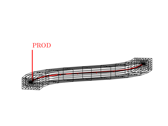
Define basic information of horizontal well (HW)

The well trajectory is specified by a set of discrete 3D well points (in xyz format) which divides the HW into multiple segments. Load well trajectory

fn = fullfile('data', 'trajectory.mat');
load(fn)
% Number of well segments
ns = size(pW,1)-1;

% Define the well structure
%  'name':         Well name, should match the well name list in deck
%  'trajectory':   Well trajectory, 3D points in xyz format
%  'segmentNum':   Number of well segment, equals to n_wellpoints - 1
%  'radius':       Wellbore (Casing) radius per well segment
%  'skinFactor':   Skin factor per well point
%  'openedSegs':   Opened segments (allow fluid to flow into the wellbore)
% The coupling of the NWM with multi-segment well requires:
%  'isMS'      :   Indicating the multi-segment well definition
%  'roughness' :   Roughness per well segment
% (See 'nearWellBoreModelingMultiSegWell')
well = struct(...
    'name'         , 'PROD', ...
    'trajectory'   , pW, ...
    'segmentNum'   , ns, ...
    'radius'       , 0.15 * ones(ns+1,1), ...
    'skinFactor'   , zeros(ns,1), ...
    'openedSegs'   , (1:ns));

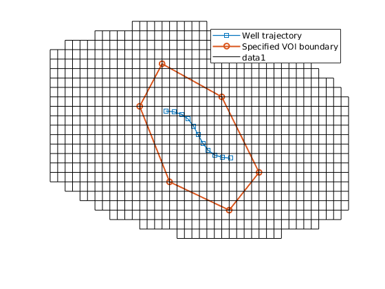
Define the volume of interest (VOI)

The VOI is a 3D region in which we will reconstruct a layered unstructured grid. Define the 2D boundary of VOI. The well should be located inside this boundary in xy plane.

pbdy = [240,   50;...
        160,   80;...
        120,  160;...
        150,  205;...
        230,  170;...
        280,   90];

% The VOI are vertically expanded by extra layers:
% nextra(1): Number of layers above the HW layers
% nextra(2): Number of layers below the HW layers
nextra = [1, 1];

% Define the VOI according to the CPG, well, boundary and extra layers
VOI = VolumeOfInterest(GC, well, pbdy, nextra);

% Get the geometrical information of CPG in VOI, including cells,
% layer-faces, boundary faces, nodes, boundary nodes, etc.
geoV = VOI.allInfoOfVolume();

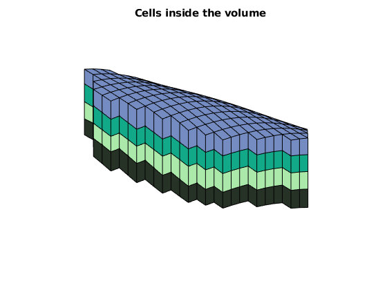
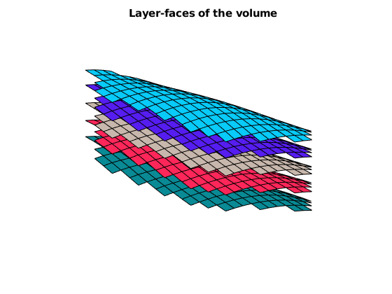
% Show the VOI boundary, cells, and faces.
VOI.plotVolumeCells(geoV), view(3)
VOI.plotVolumeLayerFaces(geoV), view(3)
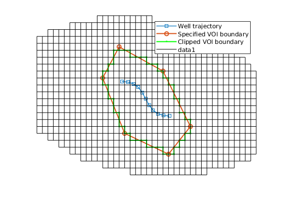
VOI.plotVolumeBoundaries(geoV), view(2)

Build the layered unstructured VOI grid

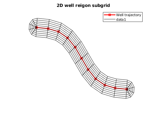
The unstructured VOI grid includes a 2D well region (WR). The WR is composed of a Cartesian region and two half-radial regions in xy plane, which is used to connect the HW grid. For the Cartesian region, the X axis extends along the well trajectory: ———> X | ———————————– Y | ——— Well trajectory ——— V ———————————–

% ly: The size of Cartesian region in Y direction, better to be larger than
% the well-segment length
% ny: The number of Cartesian cells in Y direction
% na: The number of angular cells in radial region
VOI.maxWellSegLength2D()
WR = struct('ly', 15, 'ny', 10, 'na', 5);

% Prepare the 2D well region nodes
WR = VOI.prepareWellRegionNodes2D(WR);

% Plot the 2D well region grid. This grid will be glued to the unstructured
% grid.
VOI.plot2DWRSubGrid(WR)

% Next, build the layered unstructured VOI grid. The refinement is allowed
% for each CPG layer.
% Define the number of refinement layers for each VOI layer. The dimension
% of 'layerRf' should be equal to the number of VOI layers.
VOI.volumeLayerNumber()
% Each of the four VOI layers will be refined into two sublayers.
layerRf = [2, 2, 2, 2];

% The open-source triangle generator 'DistMesh' (Per-Olof Persson) is used
% to obtain high-quality triangles. The scaled edge length function is
% defined as:
% h(p) = max(multiplier*d(p) +lIB, lOB)
% to let the point density increases from inner boundary to outer boundary
% lIB: average length of the inner boundary (outer-boundary of WR subgrid)
% lOB: average length of the outer boundary (clipped VOI boundary)

% Other parameters:
% 'maxIter' : The maximum number of distmesh iterations
% 'gridType': 'Voronoi' (default) | 'triangular'

% Reconstruct the CPG in VOI to layered unstructured grid
GV = VOI.ReConstructToUnstructuredGrid(WR, layerRf, ...
    'multiplier', 0.2, 'maxIter', 500, 'gridType', 'Voronoi');

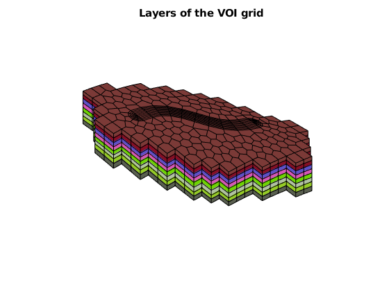
% Show the VOI grid. We can plot the specified layers / surfaces by calling
% 'GV.cells.layers==layer'/ 'GV.faces.surfaces==surface'
figure, axis off, view([-41, 62])
arrayfun(@(layer)plotGrid(GV, GV.cells.layers==layer, ...
    'facecolor', rand(3,1)), 1:GV.layers.num)
title('Layers of the VOI grid')

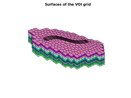
figure, axis off, view([-41, 62])
arrayfun(@(surface)plotFaces(GV, GV.faces.surfaces==surface, ...
    'facecolor', rand(3,1)), 1:GV.layers.num+1)
title('Surfaces of the VOI grid')

Info : The maximum well-segment length in 2D is 11.05
    Info : The number of VOI layers is 4 ( 4  5  6  7 )
 -- Reconstructing the CPG to unstructured VOI grid
    * Dist Mesh iteration information:
      100 iterations, 23 triangulations, tol = 0.016350
      200 iterations, 28 triangulations, tol = 0.010595
      300 iterations, 32 triangulations, tol = 0.002029
    -------------------------------------------------------------------------
...

Build the layered radial HW grid

The HW grid is built inside the Cartesian region of VOI grid. The logical indices of HW region should be specified: 1 ymin ymax ny —– —– —– —– —– —– —– | | | | | | | | 1 —– —– —– —– —– —– —– | | * | * | * | * | * | | zmin —– —– —– —– —– —– —– | | * | * | * | * | * | | —– —– —– —– —– —– —– | | * | * | * | * | * | | zmax —– —– —– —– —– —– —– | | | | | | | | nz —– —– —– —– —– —– —– * = HW region Remarks: 1 < ymin < ymax < ny (GV.surfGrid.cartDims(2)) 1 < zmin < zmax < nz (GV.layers.num)

regionIndices = [   3,    8,    2,    7];

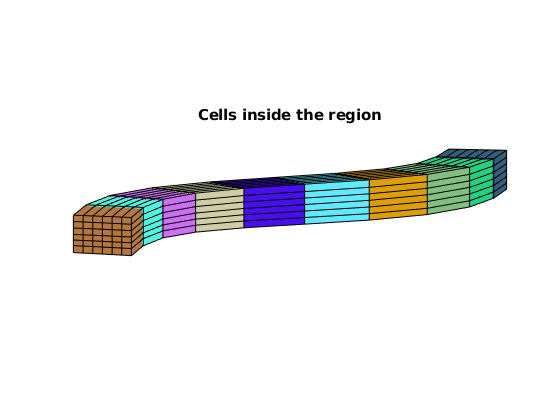
% Define the HW region according to GV, well, and regionIndices
HW = HorWellRegion(GV, well, regionIndices);

% Visualize the HW region
HW.showWellRegionInVOIGrid('showWellRgionCells', true);
view([-53, 15]), axis off
title('The HW region in VOI grid')

% Get the geometrical information of GV in HW region, including cells,
% faces, boundary faces, nodes, boundary nodes, etc.
geoW = HW.allInfoOfRegion();
HW.plotRegionCells(geoW), axis equal, view([-85, 9])
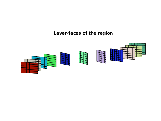
HW.plotRegionLayerFaces(geoW), axis equal, view([-85, 9])

% Next, build the layered radial HW grid. We provide two types of grid
% lines:
% Type 1: 'pureCircular'  - The radial grid lines are pure circular
% % Parameter 'maxRadius' - Max radius of the radial grid
% % Parameter 'nRadCells' - Number of radial cells
radPara1 = struct(...
    'gridType'  , 'pureCircular', ...
    'maxRadius' , 2, ...
    'nRadCells' , 8);

% Type 2: 'gradual' - The radial grid lines vary from the circular line to
%                     the rectangular line of a specified box gradually
% % Parameter 'boxRatio'  - Size ratio of the rectangular box to the outer
% %                         boundary, [yRatio, zRatio]
% % Parameter 'nRadCells' - Number of radial cells, 2x1 double,
% %                         [inbox, outbox]
% % Parameter 'pDMult'    - Multiplier of pD of the outer-most angular line
%                           to pD of wellbore line. The outer-most line
%                           will be closer to the box with increasing pDMult
% % Parameter 'offCenter' - Whether the well is off-center in the radial
% %                         grid
radPara2 = struct(...
    'gridType'  , 'gradual', ...
    'boxRatio'  , [0.6, 0.6], ...
    'nRadCells' , [7, 2], ...
    'pDMult'    , 10, ...
    'offCenter' , true);

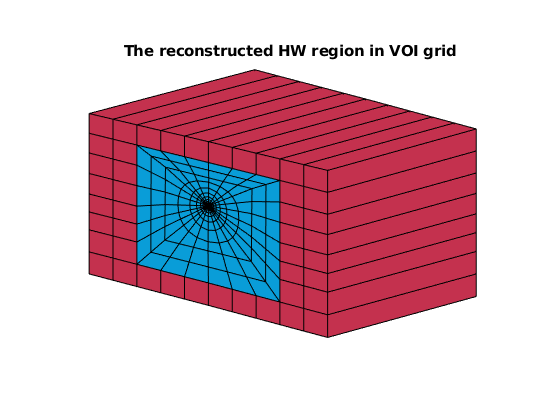
% Reconstruct the VOI grid in HW region to layered radial grid
GW = HW.ReConstructToRadialGrid(radPara2);

% Visualize the raidal grid in HW region
HW.showWellRegionInVOIGrid('showWellRgionCells', false);
plotGrid(GW, GW.cells.layers==1, 'facecolor', rand(3,1))
view([-53, 15]), axis off
title('The reconstructed HW region in VOI grid')

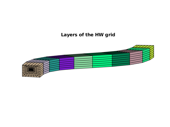
% Show the HW grid
figure, axis equal tight off, view([-85, 9])
arrayfun(@(layer)plotGrid(GW, GW.cells.layers==layer, ...
    'facecolor', rand(3,1)), 1:GW.layers.num)
title('Layers of the HW grid')

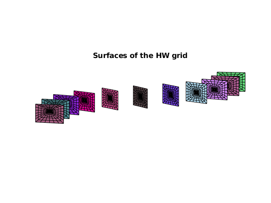
figure, axis equal tight off, view([-85, 9])
arrayfun(@(surface)plotFaces(GW, GW.faces.surfaces==surface, ...
    'facecolor', rand(3,1)), 1:GW.layers.num+1)
title('Surfaces of the HW grid')

-- Reconstructing the VOI grid to radial HW grid

Coupled model of the near-wellbore model (NWM) and multi-segment well (MSW)

Generated from nearWellBoreModelingMultiSegWell.m

This example displays the coupled model of NWM and MSW, which aims to describe both the near-wellbore flow and flow inside the wellbore. The MSW requires the node and segment definitions, which is similar to the cell and face definitions if we consider the MSW running on a virtual grid domain. Therefore, the ‘MultiSegWellNWM’ will automatically generate the node and segment definitions through building a ‘wellbore grid’. The geometrical information was obtained by grid geometries, e.g. ‘cells.centroids’, ‘cells.volumes’, and the topology of the segments corresponds to ‘faces.neighbors’. The pressure drop calculation adopts the mrst built-in wellbore friction model.

clear
mrstModule add nwm ad-core ad-blackoil ad-props mrst-gui deckformat wellpaths upr

Read the ECLIPSE input deck

fn = fullfile('data', 'MSW.data');
deck = readEclipseDeck(fn);
deck = convertDeckUnits(deck);

Build the background Cartesian grid

Here, we build a Cartesian grid as the background grid

GC = initEclipseGrid(deck);
GC = computeGeometry(GC);

Define basic information of horizontal well (HW)

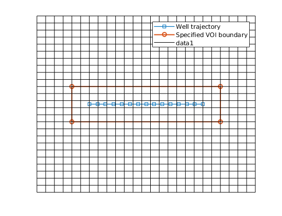
Define the well trajectory

pWx = 100*linspace(6, 19, 15)';
pWy = 100*12.5 * ones( size(pWx) );
pWz = 1050 * ones( size(pWx) );
pW = [pWx, pWy, pWz];
% Number of well segments
ns = size(pW,1)-1;
% Define the well structure
well = struct(...
    'name'         , 'PROD', ...
    'trajectory'   , pW, ...
    'segmentNum'   , ns, ...
    'radius'       , 0.1 * ones(ns+1,1), ...
    'skinFactor'   , zeros(ns,1), ...
    'openedSegs'   , 1:ns, ...
    'isMS'         , true, ...
    'roughness'    , 1e-2 * ones(ns,1));
% We set the roughness and the well production rate to quite large values
% to show the difference between MSW and simple well.

Build the layered unstructured VOI grid

Define the 2D boundary of VOI

pbdy = 100* [ 4,   10;...
             21,   10;...
             21,   15;...
              4,   15];

% Define extra layers
nextra = [1, 1];

% Define the VOI according to the CPG, well, boundary and extra layers
VOI = VolumeOfInterest(GC, well, pbdy, nextra);

% Define parameters for the 2D well region grid
VOI.maxWellSegLength2D()
WR = struct('ly', 120, 'ny', 8, 'na', 5);

% Define the number of refinement layers for each VOI layer
VOI.volumeLayerNumber()
layerRf = [2, 2, 2];

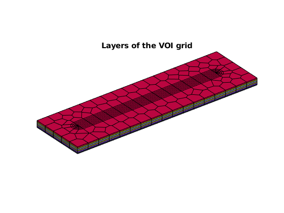
% Reconstruct the CPG in VOI to layered unstructured grid
GV = VOI.ReConstructToUnstructuredGrid(WR, layerRf, ...
    'multiplier', 0.2, 'maxIter', 500, 'gridType', 'Voronoi');

% Plot the VOI grid
figure, axis equal tight off, view(3)
arrayfun(@(layer)plotGrid(GV, GV.cells.layers==layer, ...
    'facecolor', rand(3,1)), 1:GV.layers.num)
title('Layers of the VOI grid')

Info : The maximum well-segment length in 2D is 92.86
    Info : The number of VOI layers is 3 ( 2  3  4 )
 -- Reconstructing the CPG to unstructured VOI grid
    * Dist Mesh iteration information:
      100 iterations, 25 triangulations, tol = 0.022491
      200 iterations, 32 triangulations, tol = 0.029327
      300 iterations, 38 triangulations, tol = 0.024683
      400 iterations, 44 triangulations, tol = 0.024307
...

Build the layered radial HW grid

Define the logical indices of HW region

regionIndices = [   3,    6,    2,    5];

% Define the HW region according to GV, well, and regionIndices
HW = HorWellRegion(GV, well, regionIndices);

% Define the parameters for building the radial grid
radPara = struct(...
    'gridType'  , 'gradual', ...
    'boxRatio'  , [0.6, 0.6], ...
    'nRadCells' , [10, 2], ...
    'pDMult'    , 15, ...
    'offCenter' , true);

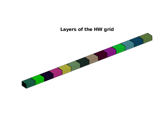
% Reconstruct the VOI grid in HW region to layered radial grid
GW = HW.ReConstructToRadialGrid(radPara);

% Plot the HW grid
figure, axis equal tight off, view(3)
arrayfun(@(layer)plotGrid(GW, GW.cells.layers==layer, ...
    'facecolor', rand(3,1)), 1:GW.layers.num)
title('Layers of the HW grid')

-- Reconstructing the VOI grid to radial HW grid

Collect the simulation data

Define the Multi-Segment well NWM by three subgrids, input deck and well

MSW = MultiSegWellNWM({GC, GV, GW}, deck, well);

% Get the global hybrid grid
G = MSW.validateGlobalGrid();

% Initialize the AD fluid
fluid = MSW.setupFluid();

% Make the subrocks
rockC = MSW.getCPGRockFromDeck();  % CPG rock
rockV = MSW.getVOIRocksByInterp(); % VOI grid rock
% Define a homogeneous rock for HW grid
rockW.perm = ones(GW.cells.num, 3) * rockC.perm(1,1);
rockW.poro = ones(GW.cells.num, 1) * 0.2;

% Get the rock for global grid
rock = MSW.getGlobalRock({rockC, rockV, rockW});

% Compute the transmissbility and neighborship
T = MSW.getTransGloGrid(rock);
intXn = MSW.computeIntxnRelation();
nnc = MSW.generateNonNeighborConn(intXn, rock, T);
[T_all, N_all] = MSW.assembleTransNeighbors(T, nnc);

% Setup simulation model
% Note the MSW model now only supports the 'ThreePhaseBlackOilModel'
model = MSW.setupSimModel(rock, T_all, N_all);

-- Computing the radial transmissibility factors
 -- Computing intersection relations between subgrids
           CPG - VOI Grid:     top boundary, elapsed time 2.61 [s]
           CPG - VOI Grid:     bot boundary, elapsed time 2.47 [s]
      VOI Grid -  HW Grid:    heel boundary, elapsed time 0.76 [s]
      VOI Grid -  HW Grid:     toe boundary, elapsed time 0.73 [s]
           CPG - VOI Grid: layered boundary, elapsed time 0.37 [s]
      VOI Grid -  HW Grid: layered boundary, elapsed time 0.15 [s]

Get the initial state by equilibrium initialization

initState = MSW.getInitState(model);

Above procedures (gridding of VOI and HW, collections of G, fluid, rock, model, and initState) are same with the basic near-wellbore model

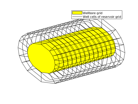
Convert the simulation schedule

We build a 1D ‘wellbore grid’ in the void wellbore space and it conforms with the reservoir grid. The wellbore grid has ‘ns’ cells (nodes) and ‘ns-1’ internal faces (segments). View the wellbore grid

gW  = MSW.wellboreGrid;
wc  = MSW.getWellCells();
figure, hold on, axis tight off
plotGrid(gW)
plotGrid(G, wc, 'facecolor', 'none')
legend('Wellbore grid', 'Well cells of reservoir grid')
view(3)

% The cells/internal faces are equivalent to the nodes/segments in the
% multi-segment well model. Each node accepts inflow from reservoir cells
% in corresponding grid layer. The segment connects its forward node and
% backward node:
%
%     o    o     o     o     o     o     o     o     o   reservoir cells
%     |    |     |     |     |     |     |     |     |   inflow to nodes
%     * -- *  -- *  -- *  -- *  -- *  -- *  -- *  -- *   nodes and segments
%     |    |     |     |     |     |     |     |     |
%     o    o     o     o     o     o     o     o     o
%
% Specially, the nodes are generated as:
%  'depth'       : gW.cells.centroids(:,3)
%  'vol'         : gW.cells.volumes
%  'cell2node'   : From grid layer indices
% The segments are generated as:
%  'topo'        : gW.faces.neighbors(internal, :)
%  'diam'        : From well info structure
%  'roughness'   : From well info structure
%  'length'      : Length between forward node and backward node
%  'flowModel'   : mrst 'wellBoreFriction' model
nodes    = MSW.generateNodes()
segments = MSW.generateSegments()
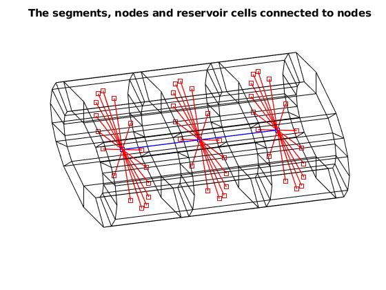
% Plot the nodes and reservoir cells associated with segment 1:2
MSW.plotSegments(nodes, segments, 1:2)
axis tight off, view([-16, 45])
title('The segments, nodes and reservoir cells connected to nodes')

% Convert the schedule from CPG to global grid
% Note the reference depth has been set to the depth of the top node
% (i.e. first cell in wellbore grid)
scheduleMS = MSW.getSimSchedule(model);

% We can also get the schedule without multi-segment well definition
schedule = MSW.getSimSchedule(model, 'returnMS', false);

% Add a flux boundary on the bottom of the grid, because there is only one
% well in the deck input
c = find(G.cells.layers==5 & G.cells.grdID==1);
fPos = mcolon(G.cells.facePos(c), G.cells.facePos(c+1));
f = G.cells.faces(fPos,:);
f = f(f(:,2)==6, 1);
v = -schedule.control.W.val / numel(f);
bc = addBC([], f, 'flux', v, 'sat', [1, 0, 0]);
scheduleMS.control.bc = bc;
schedule.control.bc = bc;

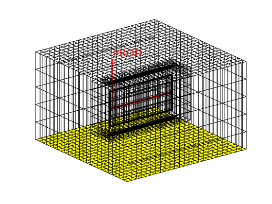
% Show the well and boundary
figure, axis tight off, view(3)
plotGrid(G, 'facecolor', 'none')
plotWell(G, schedule.control.W)
plotFaces(G, f)

nodes =

  struct with fields:

       coords: [14×3 double]
        depth: [14×1 double]
          vol: [14×1 double]
...

Run the simulations with and without multi-segment well

[wellSolsMS, statesMS, reportMS] = simulateScheduleAD(initState, model, scheduleMS);
[wellSols, states, report] = simulateScheduleAD(initState, model, schedule);

Solving timestep 01/20:                    -> 200 Days
Solving timestep 02/20: 200 Days           -> 1 Year, 35 Days
Solving timestep 03/20: 1 Year, 35 Days    -> 1 Year, 235 Days
Solving timestep 04/20: 1 Year, 235 Days   -> 2 Years, 70 Days
Solving timestep 05/20: 2 Years, 70 Days   -> 2 Years, 270 Days
Solving timestep 06/20: 2 Years, 270 Days  -> 3 Years, 105 Days
Solving timestep 07/20: 3 Years, 105 Days  -> 3 Years, 305 Days
Solving timestep 08/20: 3 Years, 305 Days  -> 4 Years, 140 Days
...

Compare the well solutions

plotWellSols({wellSols, wellSolsMS}, report.ReservoirTime)

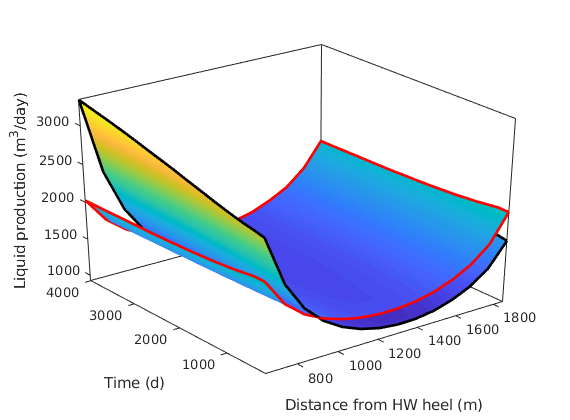
Compare the liquid production along the well

nA = GW.radDims(1);
x = ( pW(1:end-1,1) + pW(2:end,1) ) / 2;
[xx, tt] = meshgrid(x,report.ReservoirTime/day);

[fluxMS, flux] = deal( zeros(numel(wellSols), ns) );
for i = 1 : numel(wellSols)
    fMS = -sum(wellSolsMS{i}.flux,2);
    fMS = reshape(fMS, nA, []);
    fluxMS(i, :) = sum(fMS, 1);
    f = -sum(wellSols{i}.flux,2);
    f = reshape(f, nA, []);
    flux(i, :) = sum(f, 1);
end

figure,hold on
surfWithOutline(xx, tt, fluxMS/(meter^3/day));
surfWithOutline(xx, tt, flux/(meter^3/day));
hold off, box on, axis tight
shading interp
set(gca,'Projection','Perspective');
hc = get(gca, 'Children');
set(hc(1:4), 'Color', 'r')
xlabel('Distance from HW heel (m)')
ylabel('Time (d)')
zlabel('Liquid production (m^3/day)')
view(3)

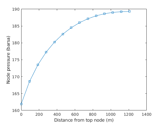
Plot the node pressures

ts = 20;
ws = wellSolsMS{ts};
nPres = [ws.bhp; ws.nodePressure];
L = nodes.coords(:,1);
L = L - L(1);
figure
plot(L, nPres/barsa, 's-')
xlabel('Distance from top node (m)')
ylabel('Node pressure (barsa)')

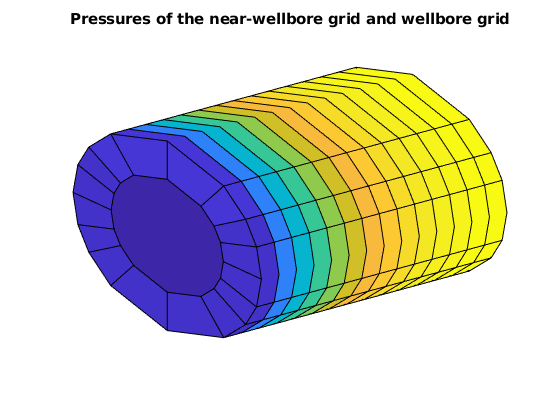
state = statesMS{end};
figure, axis tight off, view(3)
plotCellData(G, state.pressure/barsa, wc)
plotCellData(gW, nPres/barsa)
title('Pressures of the near-wellbore grid and wellbore grid')

Simulation on the Near-wellbore modeling (NWM) hybrid grid

Generated from nearWellBoreModelingSim.m

This example demonstrates how to generate necessary data structures passed to the mrst AD simulators for the NWM hybrid grid. The original data is given in ECLIPSE deck file which conforms with the background Corner-point grid (CPG). The class ‘NearWellboreModel’ accepts the data for CPG and returns the data structures for the hybrid grid in mrst standard format, consisting of ‘G’, ‘rock’, ‘fluid’, ‘model’, ‘schedule’, and ‘initState’. Before the collection, make sure that the three subgrids (GC, GV, and GW) are ready (see example ‘nearWellBoreModelingGrids’). The generation involves several key processes: * Assemble the subgrdis to get the global hybrid grid * Initialize the AD fluid * Make rocks from subones * Compute the transmissibility and neighborship (including the NNC) * Setup simulation model * Convert the simulation schedule * Define the initial state by equilibrium initialization Remarks: * In the grid domain, the subgrid boundaries are not connected. The connections between subgrids are accomplished by the non-neighbor connection (NNC). The ‘NearWellboreModel’ only accepts the ECLIPSE deck input. If you need to define the simulation data structures by mrst functionalities, e.g. ‘makeRocks’, ‘initSimpleADIFluid’, ‘addWell’, and ‘simpleSchedule’, some modifications are required. * This module now only supports the single property and equilibration region.

clear
mrstModule add nwm ad-core ad-blackoil ad-props mrst-gui diagnostics

Load subgrids, well info structure and input deck

Load subgrids (GC, GV, GW), well info structure (well), and input deck (deck) in example ‘nearWellBoreModelingGrids’

run nearWellBoreModelingGrids
close all

Info : The maximum well-segment length in 2D is 11.05
    Info : The number of VOI layers is 4 ( 4  5  6  7 )
 -- Reconstructing the CPG to unstructured VOI grid
    * Dist Mesh iteration information:
      100 iterations, 22 triangulations, tol = 0.014204
      200 iterations, 26 triangulations, tol = 0.007558
      300 iterations, 29 triangulations, tol = 0.007671
      400 iterations, 31 triangulations, tol = 0.001535
...

Define the NearWellboreModel

Define the ‘NearWellboreModel’ by three subgrids, input deck and well

NWM = NearWellboreModel({GC, GV, GW}, deck, well);

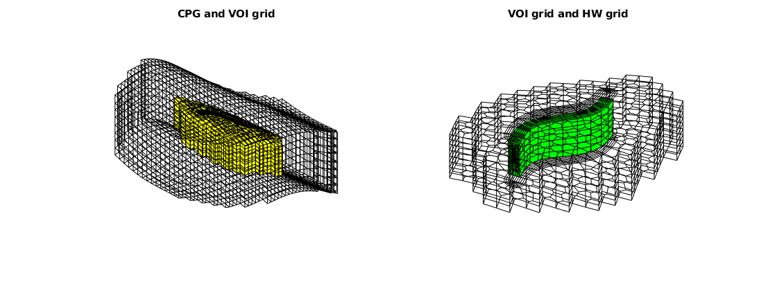
Get the global hybrid grid

G = NWM.validateGlobalGrid();

% Show the global grid. We can plot the specified subgrids by calling
% 'G.cells.grdID==i'
figure
subplot(1,2,1), hold on, axis tight off
plotGrid(G, G.cells.grdID == 1, 'facecolor', 'none')
plotGrid(G, G.cells.grdID == 2, 'facecolor', 'y')
view([-36, 38])
title('CPG and VOI grid')
subplot(1,2,2), hold on, axis tight off
plotGrid(G, G.cells.grdID == 2, 'facecolor', 'none')
plotGrid(G, G.cells.grdID == 3, 'facecolor', 'g')
view([-76, 60])
title('VOI grid and HW grid')
pos = get(gcf, 'position'); pos(3) = 2*pos(3);
set(gcf, 'position', pos);

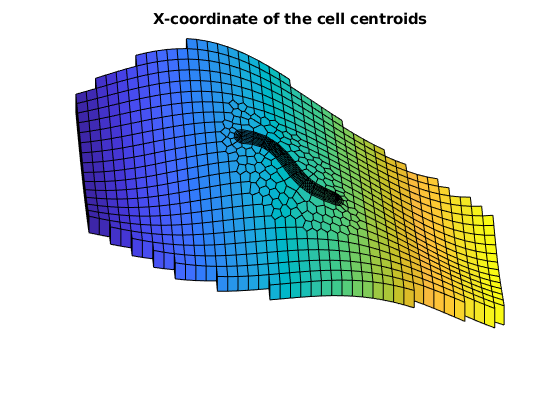
% Also, use 'G.cells.grdID == i & G.cells.layers == j' to plot layer j of
% subgrid i
figure, hold on, axis tight off
plotCellData(G, G.cells.centroids(:,1), G.cells.layers == 4 & G.cells.grdID == 1)
plotCellData(G, G.cells.centroids(:,1), G.cells.layers == 1 & G.cells.grdID == 2)
view([-3, 56])
title('X-coordinate of the cell centroids')

Initialize the AD fluid

We use ‘initDeckADIFluid’ to initialize the AD fluid

fluid = NWM.setupFluid();

Make rocks for the global grid

First, get the rocks of three subgrids: ————————————————————————- | Rock | Grid | Source | Permeability | Anisotropy | | | | | coordinate | | ----------------------------------------------------------------------- | rockC | GC | Input deck | Local | Yes | ----------------------------------------------------------------------- | rockV | GV | Interpolation | Global | Yes | | | | of rockC | | | ----------------------------------------------------------------------- | rockW | GW | User-defined | Global | No | ————————————————————————-

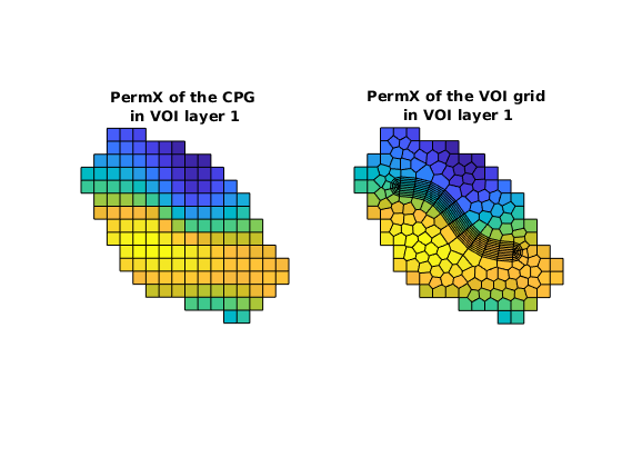
% Get rockC and rockV
rockC = NWM.getCPGRockFromDeck();
rockV = NWM.getVOIRocksByInterp();
% View rockC and rockV
figure
subplot(1,2,1), axis equal tight off
plotCellData(GC, rockC.perm(:,1), GV.parentInfo.cells{1})
title(sprintf('PermX of the CPG \nin VOI layer 1'))
subplot(1,2,2), axis equal tight off
plotCellData(GV, rockV.perm(:,1), GV.cells.layers==1)
title(sprintf('PermX of the VOI grid \nin VOI layer 1'))

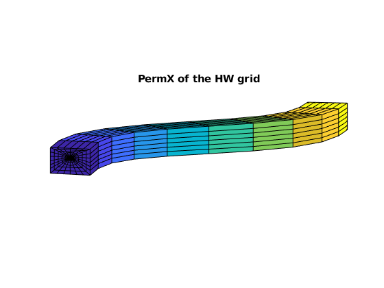
% Define a simple rock for HW grid. Each segment (layer) of the grid has
% uniform permeability and porosity
nclayer = GW.cells.num / GW.layers.num;
permW = linspace(400, 500, GW.layers.num) * (milli*darcy);
permW = repmat(permW, nclayer, 1);
poroW = linspace(0.18, 0.2, GW.layers.num);
poroW = repmat(poroW, nclayer, 1);
rockW.perm = [permW(:), permW(:), permW(:)];
rockW.poro = poroW(:);
% View rockW
figure, axis equal tight off, view([-85, 9])
plotCellData(GW, rockW.perm(:,1))
title('PermX of the HW grid')

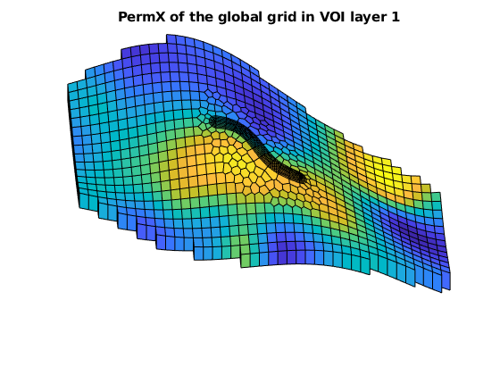
% Assemble the subrocks to get the global one
rock = NWM.getGlobalRock({rockC, rockV, rockW});
% View rock
figure, hold on, axis tight off, view([-3, 56])
plotCellData(G, rock.perm(:,1), G.cells.layers == 4 & G.cells.grdID == 1)
plotCellData(G, rock.perm(:,1), G.cells.layers == 1 & G.cells.grdID == 2)
title('PermX of the global grid in VOI layer 1')

Compute the transmissibility and neighborship

The transmissibility consists of four parts: ————————————————————————- | Trans- | Grid | Flow | Permeability | Anisotropy | | missbility | | approximation | coordinate | | ----------------------------------------------------------------------- | TC | Updated | Linear | Local | Yes | | | GC | | | | ----------------------------------------------------------------------- | TV | Updated | Linear | Global | Yes | | | GV | | | | ----------------------------------------------------------------------- | TW | GW | Radial | Global | No | | | | | | | ————————————————————————- | T_nnc | Grids | Linear | Global | Yes | | | connection | | | | ————————————————————————- * The T_nnc (transmissibility of NNC) is used to connect the subgrids * Updated GC and GV are obtained by ‘removeCells’

% Compute the transmissibility T of the global grid:
% T = [TC; TV; TW], corresponding to G.faces.neighbors
T = NWM.getTransGloGrid(rock);

% Generate the NNC
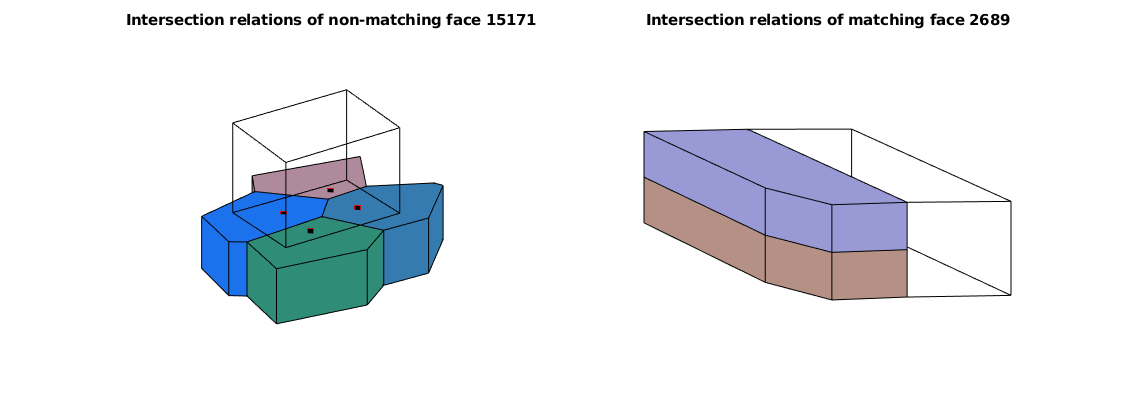
% First, compute the intersection relations between subgrids
intXn = NWM.computeIntxnRelation();
% View intersection relations
figure, subplot(1,2,1), axis off
NWM.plotNonMatchingIntxnRelation(intXn ,15171)
title('Intersection relations of non-matching face 15171')
subplot(1,2,2), axis off
NWM.plotMatchingIntxnRelation(intXn ,2689)
title('Intersection relations of matching face 2689')
pos = get(gcf, 'position'); pos(3) = 2*pos(3);
set(gcf, 'position', pos);

% Next, generate the cell pairs and associated transmissibility
nnc = NWM.generateNonNeighborConn(intXn, rock, T);

% Get the assembled transmissibility and neighborship
% T_all = [T;                 nnc.T];
% N_all = [G.faces.neighbors; nnc.cells];
[T_all, N_all] = NWM.assembleTransNeighbors(T, nnc);

-- Computing the radial transmissibility factors
 -- Computing intersection relations between subgrids
           CPG - VOI Grid:     top boundary, elapsed time 5.04 [s]
           CPG - VOI Grid:     bot boundary, elapsed time 4.60 [s]
      VOI Grid -  HW Grid:    heel boundary, elapsed time 1.68 [s]
      VOI Grid -  HW Grid:     toe boundary, elapsed time 1.25 [s]
           CPG - VOI Grid: layered boundary, elapsed time 1.17 [s]
      VOI Grid -  HW Grid: layered boundary, elapsed time 0.32 [s]

Setup simulation model

We use the ‘GenericBlackOilModel’ as the simulation model. The ‘neighbors’ and ‘trans’ in model.operators are rewritten: model.operators = setupOperatorsTPFA(G, rock,’neighbors’, N, ‘trans’, T); model.operators.T_all = T_all;

model = NWM.setupSimModel(rock, T_all, N_all);

Convert the simulation schedule

Convert the schedule from the section ‘SCHEDULE’ in deck for the global grid. Some fields in ‘W’ of the HW are redefined, e.g. ‘cells’, ‘WI’.

schedule = NWM.getSimSchedule(model, 'refDepthFrom', 'deck');

% Show the well
figure, axis equal tight off, view([-85, 9])
plotGrid(G, G.cells.grdID == 3, 'facecolor', 'none')
plotWell(G, schedule.control(1).W(1))

-- Converting schedule from input deck
    Info : The reference depth of PROD adopts the value from deck
    Info : The reference depth of PROD adopts the value from deck

Get the initial state by equilibrium initialization

initState = NWM.getInitState(model);

Run the simulation

[wellSols, states, report] = simulateScheduleAD(initState, model, schedule);

Solving timestep 01/20:         -> 2 Days
Solving timestep 02/20: 2 Days  -> 4 Days
Solving timestep 03/20: 4 Days  -> 6 Days
Solving timestep 04/20: 6 Days  -> 8 Days
Solving timestep 05/20: 8 Days  -> 10 Days
Solving timestep 06/20: 10 Days -> 12 Days
Solving timestep 07/20: 12 Days -> 14 Days
Solving timestep 08/20: 14 Days -> 16 Days
...

Plot the results

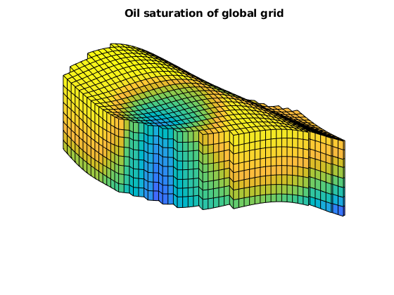
Oil saturation

ts = 20;
state = states{ts};

figure, axis tight off, view([-23, 29])
plotCellData(G, state.s(:,2))
title('Oil saturation of global grid')

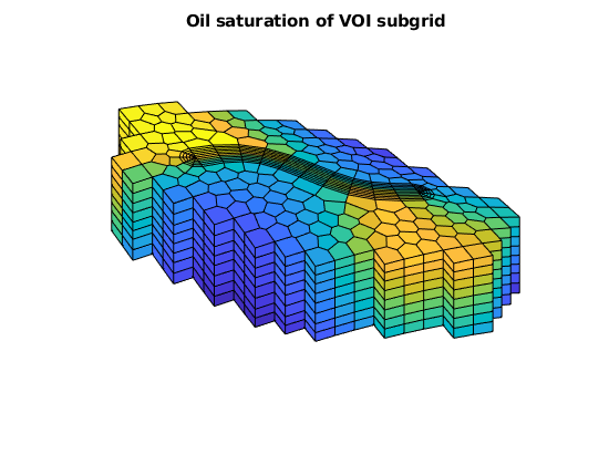
figure, axis tight off, view([-27, 56])
plotCellData(G, state.s(:,2), G.cells.grdID==2)
title('Oil saturation of VOI subgrid')

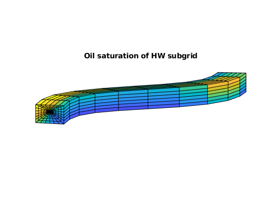
figure, axis equal tight off, view([-85, 9])
plotCellData(G, state.s(:,2), G.cells.grdID==3)
title('Oil saturation of HW subgrid')

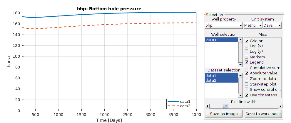
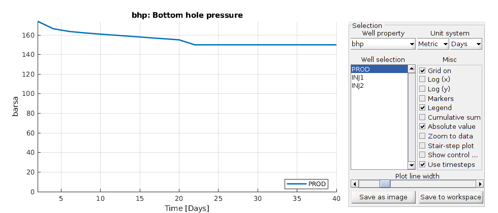
% Well solutions
plotWellSols(wellSols, report.ReservoirTime)

Apply some flow diagnostics

Since the NNC is introduced to operators, we should rearrange the output flux

flux0 = state.flux;
flux0 = flux0(~all(flux0==0, 2), :);
flux = zeros(size(N_all,1), 3);
intCon = all(N_all, 2);
flux(intCon, :) = flux0;
state.flux = flux;

% Define a temporary 'G' whose 'faces.neighbors' are replaced by N_all to
% be compatible with 'computeTimeOfFlight'
Gtmp = G;
Gtmp.faces.neighbors = N_all;

% Compute TOF and tracer partitioning
W = schedule.control(2).W;
D = computeTOFandTracer(state, Gtmp, rock, 'wells', W);

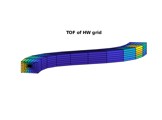
% Visualize the TOF of HW subgrid
figure, axis equal tight off, view([-85, 9])
plotCellData(G, sum(D.tof,2), G.cells.grdID == 3)
title('TOF of HW grid')

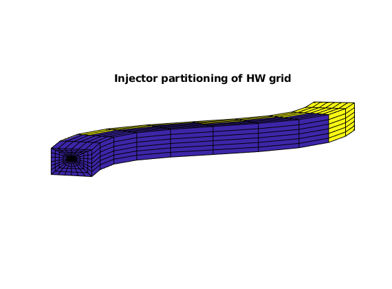
% Visualize the injector partitioning of HW subgrid
figure, axis equal tight off, view([-85, 9])
plotCellData(G, D.ipart, G.cells.grdID == 3)
title('Injector partitioning of HW grid')

Near-wellbore modeling (NWM) workflow example

Generated from nearWellBoreModelingWorkFlow.m

This example aims to show the complete workflow for the NWM method. This includes building the volume of interest (VOI) grid, building the horizontal well (HW) grid, and generating data structures passed to the AD simulators. Details about the grids and data structure generations can be found in example ‘nearWellBoreModelingGrids’ and ‘nearWellBoreModelingSim’, respectively.

clear
mrstModule add nwm ad-core ad-blackoil ad-props mrst-gui deckformat wellpaths upr

Read the ECLIPSE input deck

fn = fullfile('data', 'NWM.data');
deck = readEclipseDeck(fn);
deck = convertDeckUnits(deck);

Build the background Corner-point grid (CPG)

GC = initEclipseGrid(deck);
GC = computeGeometry(GC);

Define basic information of horizontal well (HW)

Load well trajectory

fn = fullfile('data', 'trajectory.mat');
load(fn)
% Number of well segments
ns = size(pW,1)-1;
% Define the well structure
well = struct(...
    'name'         , 'PROD', ...
    'trajectory'   , pW, ...
    'segmentNum'   , ns, ...
    'radius'       , 0.15 * ones(ns+1,1), ...
    'skinFactor'   , zeros(ns,1), ...
    'openedSegs'   , (1:ns));

Build the layered unstructured VOI grid

Define the 2D boundary of VOI

pbdy = [240,   50;...
        160,   80;...
        120,  160;...
        150,  205;...
        230,  170;...
        280,   90];

% Define extra layers
nextra = [1, 1];

% Define the VOI according to the CPG, well, boundary and extra layers
VOI = VolumeOfInterest(GC, well, pbdy, nextra);

% Define parameters for the 2D well region subgrid
VOI.maxWellSegLength2D()
WR = struct('ly', 15, 'ny', 10, 'na', 5);

% Define the number of refinement layers for each VOI layer
VOI.volumeLayerNumber()
layerRf = [2, 2, 2, 2];

% Reconstruct the CPG in VOI to layered unstructured grid
GV = VOI.ReConstructToUnstructuredGrid(WR, layerRf, ...
    'multiplier', 0.2, 'maxIter', 500, 'gridType', 'Voronoi');

Info : The maximum well-segment length in 2D is 11.05
    Info : The number of VOI layers is 4 ( 4  5  6  7 )
 -- Reconstructing the CPG to unstructured VOI grid
    * Dist Mesh iteration information:
      100 iterations, 22 triangulations, tol = 0.027767
      200 iterations, 29 triangulations, tol = 0.008897
      300 iterations, 32 triangulations, tol = 0.010805
      400 iterations, 37 triangulations, tol = 0.010302
...

Build the layered radial HW grid

Define the logical indices of HW region

regionIndices = [   3,    8,    2,    7];

% Define the HW region according to the GV, well, and regionIndices
HW = HorWellRegion(GV, well, regionIndices);

% Define the parameters for building the radial grid
radPara = struct(...
    'gridType'  , 'gradual', ...
    'boxRatio'  , [0.6, 0.6], ...
    'nRadCells' , [7, 2], ...
    'pDMult'    , 10, ...
    'offCenter' , true);

% Reconstruct the VOI grid in HW region to layered radial grid
GW = HW.ReConstructToRadialGrid(radPara);

-- Reconstructing the VOI grid to radial HW grid

Generate data structures for the AD simulator

Define the ‘NearWellboreModel’ by three subgrids, input deck and well

NWM = NearWellboreModel({GC, GV, GW}, deck, well);

% Define a simple rock for HW grid
nclayer = GW.cells.num / GW.layers.num;
permW = linspace(400, 500, GW.layers.num) * (milli*darcy);
permW = repmat(permW, nclayer, 1);
poroW = linspace(0.18, 0.2, GW.layers.num);
poroW = repmat(poroW, nclayer, 1);
rockW.perm = [permW(:), permW(:), permW(:)];
rockW.poro = poroW(:);

% Get the mrst data structures for the NWM grid
[G, rock, fluid, model, schedule, initState] = NWM.packedSimData(rockW);

% Get the mrst data structures for the CPG
[GC, rockC, ~, modelC, scheduleC, initStateC] = NWM.packedCPGSimData();

-- Computing the radial transmissibility factors
 -- Computing intersection relations between subgrids
           CPG - VOI Grid:     top boundary, elapsed time 3.87 [s]
           CPG - VOI Grid:     bot boundary, elapsed time 3.79 [s]
      VOI Grid -  HW Grid:    heel boundary, elapsed time 1.07 [s]
      VOI Grid -  HW Grid:     toe boundary, elapsed time 1.08 [s]
           CPG - VOI Grid: layered boundary, elapsed time 1.00 [s]
      VOI Grid -  HW Grid: layered boundary, elapsed time 0.29 [s]
...

Run the simulation

[wellSols, states, report] = simulateScheduleAD(initState, model, schedule);

Solving timestep 01/20:         -> 2 Days
Solving timestep 02/20: 2 Days  -> 4 Days
Solving timestep 03/20: 4 Days  -> 6 Days
Solving timestep 04/20: 6 Days  -> 8 Days
Solving timestep 05/20: 8 Days  -> 10 Days
Solving timestep 06/20: 10 Days -> 12 Days
Solving timestep 07/20: 12 Days -> 14 Days
Solving timestep 08/20: 14 Days -> 16 Days
...

Example of connecting the well-region grid to Cartesian grid by the Voronoi grid

Generated from connWRCartGrids.m

This example demonstrates the use of Voronoi (pebi) grid to connect the well-region (WR) grid to Cartesian grid. The Voronoi grid is constructed by the combination of ‘voronoin’ (provides grid nodes and connectivity list) and ‘tessellationGrid’, before which five special treatments are conducted, i.e. * Designing the generating points * Clipping the Voronoi diagram * Removing conflicting points * Connecting with the WR grid * Connecting with the Cartesian grid

clear
mrstModule add nwm upr ad-core ad-props ad-blackoil diagnostics

Build the Cartesian grid

GC = cartGrid([25, 25], [200, 200]);
GC = computeGeometry(GC);

Define well trajectory and region of interest (ROI) boundary

The well trajectory, should be located inside the ROI boundary.

ns = 12;
th = linspace(0.85, 0.7, ns+1)' * pi;
traj = [150*cos(th)+200, 150*sin(th)];
% The polygonal ROI boundary
pbdy = [136, 150;
        145,  95;
         90,  30;
         35,  45;
         45, 105;
         90, 160];

% Get cells inside and outside the ROI
cCtro = GC.cells.centroids;
in = inpolygon(cCtro(:,1), cCtro(:,2), pbdy(:,1), pbdy(:,2));
cI = find( in );
cO = find(~in );

% Extract the sorted boundary nodes and boundary cells (in counterclockwise).
% The actual ROI boundary is aligned to the grid edges (faces) and
% therefore lead the nonconvex polygons. So, we first sort the convex
% polygon specified by the centroids of boundary edges, and then obtain the
% sorted boundary nodes and cells from associated faces.
[bnC, bcC] = extractBdyNodesCells(GC, cI);

% Plot the ROI boundary
figure, hold on, axis equal tight off
plotGrid(GC, cO, 'facecolor', 'none')
plotGrid(GC, cI, 'facecolor', 'y')
demoPlotLine(traj, 'ko-', 'b', 4)
demoPlotPoly(pbdy, 'k^-', 'r', 5)
demoPlotPoly(GC.nodes.coords(bnC,:), 'ks-', 'g', 4)
legend('GC outside the ROI', 'GC inside the ROI', 'Well path' ,...
    'Specified ROI boundary','Clipped ROI boundary')

Get the points and connectivity list of WR grid

The WR grid is built along the well trajectory, consisting of a Cartesian region and two half-radial regions. For the Cartesian region, the X axis extends along the well trajectory. (see ‘nearWellBoreModelingGrids’)

% The number of Cartesian cells in Y direction
ny = 8;
% The size Cartesian region in Y direction
ly = 12;
% The number of angular cells in radial region
na = 6;
% Generate the WR grid points
pW0 = arrayfun(@(ii)pointsSingleWellNode(traj, ly, ny, na, ii), (1:ns+1)');
pW  = [vertcat(pW0.cart); vertcat(pW0.rad)];
% Make sure that all well-region points are located inside the ROI
assert( all(inpolygon(pW(:,1), pW(:,2), GC.nodes.coords(bnC,1), ...
    GC.nodes.coords(bnC,2))) );
% Get the connectivity list and boundary nodes
[tW, ~, bnW] = getConnListAndBdyNodeWR2D(pW0, ny, na);
% Build the WR grid
GW = tessellationGrid(pW, tW);

figure, hold on, axis equal tight off
plotGrid(GC, cO, 'facecolor', 'none')
plotGrid(GW, 'facecolor', [.0, .44, .74])
demoPlotPoly(GC.nodes.coords(bnC, :), 'ks-', 'g', 4)
demoPlotPoly(pW(bnW, :), 'ko-', 'y', 3)
legend('GC outside the ROI', 'GW (WR grid)', 'ROI boundary' ,'WR boundary')

Design the generating points

The Voronoi grid is built within the region between the outer boundary (ROI boundary) and inner boundary (WR grid boundary), namely transition region (TR) here. The nodes of the Voronoi grid should locate the nodes of outer and inner boundaries. Therefore, the generating points should be designed. Here, the generating point set consist of the basic point set and the auxiliary point set.

% The basic points are generated by 'DistMesh' (Per-Olof Persson) within
% the reduced TR. The outer boundary of reduced TR is specified by the
% centroids of boundary cells (bcC), and the inner boundary is specified
% the intersection points (outside the WR grid) of circumcircles of the WR
% boundary nodes.

% The boundaries of TR
pob  = GC.nodes.coords(bnC,:);
pib  = pW(bnW, :);

% The boundaries of reduced TR
pob2 = GC.cells.centroids(bcC, :);
[pIn, pOut, R] = demoComputeAuxPts(pW, bnW, 0.35);
pib2 = pOut;

% Plot the boundaries
figure, hold on, axis equal tight off
demoPlotPoly(pob,  'ks-', 'g', 4)
demoPlotPoly(pib,  'ko-', 'y', 3)
demoPlotPoly(pob2, 'ks-', 'r', 4)
demoPlotPoly(pib2, 'ko-', 'b', 3)
legend('Outer boundary of TR' ,'Inner boundary of TR', ...
    'Outer boundary of reduced TR' ,'Inner boundary of reduced TR')

% Generate basic points by 'Distmesh'
[pdis, tdis] = passToDistmesh(pib2, pob2, 0.2, 500, 'pIBRadius', R);

% The auxiliary points consist of the centroids of the Cartesian cells
% outside the ROI and the intersection points (inside the WR grid) of
% circumcircles of the WR boundary nodes.
pauxW = pIn;
pauxC = GC.cells.centroids(cO, :);

% Combine the basic points and auxiliary points to get the generating
% points of the Voronoi diagram
pall = [pdis; pauxC; pauxW];
% Get the nodes and connectivity list of the Voronoi diagram
[pVor, tVor] = voronoin(pall, {'Qbb','Qz'});

% Plot the Voronoi diagram
figure, hold on, axis equal off
voronoi(pall(:,1), pall(:,2), '-')
demoPlotPoly(pdis,  'ro',  'r', 2)
demoPlotPoly(pauxC, 'bo',  'b', 2)
demoPlotPoly(pauxW, 'k^',  'k', 3)
demoPlotPoly(pob,   'ks-', 'g', 4)
demoPlotPoly(pib,   'ko-', 'y', 3)
legend('', 'Initial Voronoi digram', 'Basic points' ,'Auxiliary points (CO)', ...
    'Auxiliary points (WR)', 'Outer boundary of TR' ,'Inner boundary of TR')
xlim([-20, 220])
ylim([-20, 220])

* Dist Mesh iteration information:
      100 iterations, 24 triangulations, tol = 0.020603
      200 iterations, 31 triangulations, tol = 0.005153

Handle the Voronoi diagram

Here, three treatments are performed: * Clipping the Voronoi diagram * Removing conflicting points * Connecting with the WR grid

[pVor, tVor, bnVor] = demoHandleVoronoiDiag(pVor, tVor, pib, pob, pW, tW, bnW);

Connect with the Cartesian grid

Next, connect the Voronoi grid (already connected to the WR grid) with the Cartesian grid Remove cells inside the ROI

[GC_Rem, ~, ~, mapn] = removeCells(GC, cI);
pC = GC_Rem.nodes.coords;

% Get the indices of boundary nodes in GC_Rem
bnC = arrayfun(@(n)find(mapn == n), bnC);

% Merge the common nodes (boundary nodes). The boundary node indices in pC
% are replaced by the ones in pVor
nNo  = (1:size(pC,1))';
% The non-boundary nodes indices
idx  = ~ismember(nNo, bnC);
nNo(idx) = (1:nnz(idx))' + size(pVor,1);
pC = pC(idx,:);
% We already know the boundary nodes in pVor: bnVor
nNo(bnC)  = bnVor;

% Map the connectivity list of GC_Rem
[cnC, pos] = gridCellNodes(GC_Rem, (1:GC_Rem.cells.num));
cnC = nNo(cnC);
tC  = arrayfun(@(c)cnC(pos(c):pos(c+1)-1), (1:GC_Rem.cells.num)', ...
    'UniformOutput', false);

Get the hybrid grid

Assemble the points and connectivity lists

p = [pVor; pC];
t = [tVor; tC];
t = sortPtsCounterClockWise(p, t);

% Build the hybrid grid
G = tessellationGrid(p, t);
G = computeGeometry(G);

figure, hold on, axis equal tight off
plotGrid(G)

Run simulation on the hybrid grid

Define a two phase (oil-water) fluid

fluid = initSimpleADIFluid('mu',    [1, 5, 0]*centi*poise, ...
                           'rho',   [1000, 700, 0]*kilogram/meter^3, ...
                           'n',     [2, 2, 0],...
                           'c',     [1e-5, 1e-4, 0] * (barsa)^(-1));

% Make rock
rock = makeRock(G, [.25, .25]*darcy, 0.25);
% Let the permeability of WR be higher
idx = (1:size(tW,1))'; % The cell indices of WR
rock.perm(idx, :) = rock.perm(idx, :) * 20;
% Plot the X permeability
figure, hold on; axis equal off
plotCellData(G, rock.perm(:,1))
title('X permeability')

% Setup simulation model
model = TwoPhaseOilWaterModel(G, rock, fluid);

% Define the wells
% Injector, south-west corner cell
D = sqrt( sum(G.cells.centroids.^2, 2) );
wcI = find( D==min(D) );
W = addWell([], G, rock, wcI, 'Name', 'INJ', 'sign', 1, ...
    'comp_i', [1, 0], 'Val', 10*(meter^3/day), 'Type', 'rate');

% Producer, north-east corner cell
wcP = find( D==max(D) );
W = addWell(W, G, rock, wcP, 'Name', 'PROD', 'sign', -1, ...
    'comp_i', [1, 1], 'Val', 100*(barsa), 'Type', 'bhp');

% Plot the well cells
figure, hold on; axis equal off
plotGrid(G, 'facecolor', 'none')
plotGrid(G, W(1).cells, 'facecolor', 'r')
plotGrid(G, W(2).cells, 'facecolor', 'b')
legend('G', 'Injector cell', 'Producer cell')

% Define the schedule
timesteps = ones(20,1)*30*day;
schedule  = simpleSchedule(timesteps, 'W', W);

% Define the initial state
sW = zeros(G.cells.num, 1);
sat = [sW, 1 - sW];
state0 = initResSol(G, 300*barsa, sat);

% Run the simulation
[wellSols, states, report] = simulateScheduleAD(state0, model, schedule);

Solving timestep 01/20:                  -> 30 Days
Solving timestep 02/20: 30 Days          -> 60 Days
Solving timestep 03/20: 60 Days          -> 90 Days
Solving timestep 04/20: 90 Days          -> 120 Days
Solving timestep 05/20: 120 Days         -> 150 Days
Solving timestep 06/20: 150 Days         -> 180 Days
Solving timestep 07/20: 180 Days         -> 210 Days
Solving timestep 08/20: 210 Days         -> 240 Days
...

Plot the results

Well solutions

plotWellSols(wellSols, report.ReservoirTime)

% Oil saturation
ts = 20;
state = states{ts};
figure
subplot(1,3,1), axis equal tight off
plotCellData(G, state.s(:,2), 'edgecolor', 'none')
title('Oil saturation')
% Pressure
subplot(1,3,2), axis equal tight off
plotCellData(G, state.pressure/barsa, 'edgecolor', 'none')
title('Pressure')
% TOF
W = schedule.control.W;
D = computeTOFandTracer(state, G, rock, 'wells', W);
subplot(1,3,3), axis equal tight off
plotCellData(G, D.tof(:,1), 'edgecolor', 'none')
title('TOF from injector')

Demonstration of gluing the radial grid to Cartesian grid

Generated from glueRadCartGrids.m

This example demonstrates how to build the hybrid grid by gluing the radial grid in the near-well region to the Cartesian grid elsewhere in the reservoir. The use of the constructor ‘tessellationGrid’ makes it easy to connect the two subgrids: obtain the points and connectivity lists of the subgrids and then assemble them to get the global ones. In addition, the common points at the grid boundaries are merged and mapped.

clear
mrstModule add nwm

Build the Cartesian grid

GC = cartGrid([20, 20], [200, 200]);
GC = computeGeometry(GC);

% Define the well region by logical indices
% 10 <= i <= 14
% 10 <= j <= 14
ij = gridLogicalIndices(GC);
idxI = ij{1} >= 10 & ij{1} <= 14 & ij{2} >= 10 & ij{2} <= 14;

% Cells inside the region
cI = find(idxI);
% Cells outside the region
cO = find(~idxI);

% Plot the cells
figure, hold on; axis equal off
plotGrid(GC, cO, 'facecolor', 'y')
plotGrid(GC, cI, 'facecolor', 'g')
legend('Cells outside the well reigon', 'Cells inside the well reigon')

% Extract the sorted boundary nodes of the reigon (in counterclockwise)
bn = extractBdyNodesCells(GC, cI);

Generate radial point set

nA - Number of cells in angular direction nR - Number of cells in radial direction rW - The minimum radius rM - The maximum radius

% The angular dimension and grid angles are determined by the boundary
% nodes to conform with the Cartesian grid
nA = numel(bn);

% Place the well at the region center
pCI = GC.cells.centroids(cI, :);
pW  = 0.5*[min(pCI(:,1)) + max(pCI(:,1)), min(pCI(:,2)) + max(pCI(:,2))];
pbn  = GC.nodes.coords(bn, :);
pbn0 = bsxfun(@minus, pbn, pW);

% Compute the angles
th = cart2pol(pbn0(:,1), pbn0(:,2));

% Define the logarithmic grid radii
[nR, rW, rM] = deal(10, 0.2, 16);
r = logspace(log10(rW), log10(rM), nR+1);

% Get the radial grid points
[R, TH] = meshgrid(r, th);
[px, py] = pol2cart(TH(:), R(:));
pR = bsxfun(@plus, [px(:), py(:)], pW);

% The boundary points are the outermost angular points. The total radial
% dimension is then nR+1
pR = [pR; pbn];

Build the radial grid

[GR, tR] = buildRadialGrid(pR, nA, nR+1);

% Plot the radial grid
figure, hold on; axis equal off
plotGrid(GC, cO, 'facecolor', 'y')
plotGrid(GR, 'facecolor', 'g')
legend('Cells outside the well reigon', 'Cells inside the well reigon')

Glue the grids

The constructor ‘tessellationGrid’ is used to glue the two grids. First, we should get the points and connectivity lists of the two subgrids. The connectivity list provides the indices of nodes specifying each polygonal cell, i.e. the nodes of cells.

% Points and connectivity list of the radial grid
pR = GR.nodes.coords;
% tR is obtained from 'buildRadialGrid' to keep consistency of indices

% Points and connectivity list of the Cartesian grid
% Remove the cells inside the well region first
[GC_Rem, ~, ~, mapn] = removeCells(GC, cI);
pC = GC_Rem.nodes.coords;

% Get the indices of boundary nodes in GC_Rem
bn = arrayfun(@(n)find(mapn == n), bn);

% Merge the common nodes (boundary nodes). The boundary node indices in pC
% are replaced by the ones in pR
nNo  = (1:size(pC,1))';
% The non-boundary nodes indices
idx  = ~ismember(nNo, bn);
nNo(idx) = (1:nnz(idx))' + size(pR,1);
pC = pC(idx,:);
% We already know the bounday nodes in pR: the last nA nodes
nNo(bn)  = size(pR,1)+1 - (nA:-1:1)';

% Map the connectivity list of GC_Rem
[cnC, pos] = gridCellNodes(GC_Rem, (1:GC_Rem.cells.num));
cnC = nNo(cnC);
tC  = arrayfun(@(c)cnC(pos(c):pos(c+1)-1), (1:GC_Rem.cells.num)', ...
    'UniformOutput', false);

% Assemble the points and connectivity lists
p = [pR; pC];
% Sort the tC to same direction with tR (in clockwise)
tC = sortPtsClockWise(p, tC);
t = [tR; tC];

% Build the hybrid grid
G = tessellationGrid(p, t);
G = computeGeometry(G);

% Plot the hybrid grid
figure, hold on; axis equal off
plotGrid(G)

The function ‘radCartHybridGrid’ integrates above generation process, we can call it to build a hybrid grid directly.

G1 = radCartHybridGrid(GC, cI, rW, rM, nR, pW)

G1 =

  struct with fields:

       faces: [1×1 struct]
       cells: [1×1 struct]
       nodes: [1×1 struct]
...

Example of simulation on a radial-Cartesian hybrid grid

Generated from simRadCartGrids.m

This example demonstrates how to perform simulation on a radial-Cartesian hybrid grid. The additional treatments for such grid involve the calculation of radial transmissibility and the definition of the well structure. Also, the simulation performances between the standalone Cartesian grid that uses the Peaceman well model and the hybrid grid are compared.

clear
mrstModule add nwm ad-core ad-blackoil ad-props

Build the hybrid grid

Build the Cartesian grid

GC = cartGrid([15, 15], [1000, 1000]);
GC = computeGeometry(GC);

% Define the well region by logical indices
ij = gridLogicalIndices(GC);
idxI = ij{1} >= 6 & ij{1} <= 10 & ij{2} >= 6 & ij{2} <= 10;
cI = find(idxI);

% Place the well at the region center
pW  = [500, 500];

% Define radial parameters
[nR, rW, rM] = deal(10, 0.2, 100);

% Get the hybrid grid
G = radCartHybridGrid(GC, cI, rW, rM, nR, pW);
figure, hold on; axis equal off, plotGrid(G)

Compute the radial half transmissibility factor

The radial transmissibility is derived from the radial/angular two-point flux approximation. The derivation assumes the steady-state flow and computes ‘transmissibility center’ by integral of the pressure within the area of cell. The half transmissibility = permeability .* factor.

% Assign the radial grid
GR = G.subGrids{1};
% The irregular outermost radial cells are not involved in the calculations
GR.radDims = [GR.radDims(1), GR.radDims(2)-1, 1];

% Compute the factor
skin = 0;
ft = computeRadTransFactor(GR, pW, skin);
ft = ft(~isnan(ft));

Assign the radial transmissibility

Define a homogeneous rock

rock = makeRock(G, [.25, .25]*darcy, 0.25);

% Linear half transmissibility
hT = computeTrans(G, rock);

% Indices of radial cells involved in the factor calculations
radCells = (1:GR.cells.num-GR.radDims(1))';

% Note the factor is suitable for only isotropic permeability
permR = rock.perm(radCells,1);
n = diff(G.cells.facePos);
permR = rldecode(permR, n(radCells));

% Compute the radial half transmissibility
hTR = permR .* ft;

% Assign the radial half transmissibility
idx = (1:numel(hTR))';
hT(idx) = hTR;

% Compute the full transmissibility
cf = G.cells.faces(:,1);
nf = G.faces.num;
assert( numel(hT) == numel(cf) )
T_all  = 1 ./ accumarray(cf, 1./hT, [nf, 1]);
intCon = all(G.faces.neighbors, 2);
T = T_all(intCon);

Setup simulation model

Define a two phase (oil-water) fluid

fluid = initSimpleADIFluid('mu',    [1, 5, 0]*centi*poise, ...
                           'rho',   [1000, 700, 0]*kilogram/meter^3, ...
                           'n',     [2, 2, 0],...
                           'c',     [1e-5, 1e-3, 0] * (barsa)^(-1));

% Setup the simulation model
model  = TwoPhaseOilWaterModel(G,  rock, fluid);
% Rewrite the transmissibilities
model.operators.T_all = T_all;
model.operators.T = T;

% The rock and model of Cartesian grid
rockC  = makeRock(GC, [.25, .25]*darcy, 0.25);
modelC = TwoPhaseOilWaterModel(GC, rockC, fluid);

Define wells for the hybrid grid

Setup two injectors INJ1: south-west corner cell INJ2: north-east corner cell

D = sqrt( sum(G.cells.centroids.^2, 2) );
wcI = [find( D==min(D) ), find( D==max(D) )];
rate = 100*(meter^3/day);
W = [];
for j = 1 : 2
    W = addWell(W, G, rock, wcI(j), 'Name', sprintf('INJ%d',j), ...
        'sign', 1, 'comp_i', [1, 0], 'Val', rate, 'Type', 'rate');
end

% Producer in the hybrid grid
% Find the wellbore face first
D = bsxfun(@minus, G.faces.centroids, pW);
D = sqrt(sum(D.^2,2));
wf = find(~all(G.faces.neighbors,2) & D < 1.5*rW);
% The well index is the half transmissibility (radial) of the wellbore face
WI = T_all(wf);
% Get the well cells
wcP = sum(G.faces.neighbors(wf,:), 2);
bhp = 50*barsa;
W = addWell(W, G, rock, wcP, 'Name', 'PROD', 'sign', -1, ...
    'comp_i', [1, 1], 'Val', bhp, 'Type', 'bhp', 'WI', WI);

% Plot the well cells
figure, hold on; axis equal off
plotGrid(G, 'facecolor', 'none')
plotGrid(G, W(3).cells)
xlim([498,502]); ylim([498,502]);
legend('G', 'Well cells')

Define wells for the Cartesian grid

Setup two injectors INJ1: south-west corner cell INJ2: north-east corner cell

D = sqrt( sum(GC.cells.centroids.^2, 2) );
wcI = [find( D==min(D) ), find( D==max(D) )];
WC = [];
for j = 1 : 2
    WC = addWell(WC, GC, rockC, wcI(j), 'Name', sprintf('INJ%d',j), 'sign', 1, ...
        'comp_i', [1, 0], 'Val', rate, 'Type', 'rate');
end

% Producer
D = bsxfun(@minus, GC.cells.centroids, pW);
D = sqrt(sum(D.^2,2));
wcP = find(D==min(D));
WC = addWell(WC, GC, rockC, wcP, 'Name', 'PROD', 'sign', -1, ...
    'comp_i', [1, 1], 'Val', bhp, 'Type', 'bhp', 'Radius', rW);

Define the schedule

timesteps = ones(20,1)*30*day;
schedule  = simpleSchedule(timesteps, 'W', W);
scheduleC = simpleSchedule(timesteps, 'W', WC);

Define the initial state

sW = zeros(G.cells.num, 1);
sat = [sW, 1 - sW];
state0 = initResSol(G, 300*barsa, sat);

sW = zeros(GC.cells.num, 1);
sat = [sW, 1 - sW];
state0C = initResSol(GC, 300*barsa, sat);

Run the simulation

[wellSols, states, report] = simulateScheduleAD(state0, model, schedule);
[wellSolsC, statesC, reportC] = simulateScheduleAD(state0C, modelC, scheduleC);

Solving timestep 01/20:                  -> 30 Days
Solving timestep 02/20: 30 Days          -> 60 Days
Solving timestep 03/20: 60 Days          -> 90 Days
Solving timestep 04/20: 90 Days          -> 120 Days
Solving timestep 05/20: 120 Days         -> 150 Days
Solving timestep 06/20: 150 Days         -> 180 Days
Solving timestep 07/20: 180 Days         -> 210 Days
Solving timestep 08/20: 210 Days         -> 240 Days
...

Compare the well solutions

Show the differences of producer’s data (bhp, qWs, qOs) between the hybrid grid and Cartesian grid

plotWellSols({wellSols, wellSolsC}, report.ReservoirTime)

Compare the pressure and oil saturation

ts = 20;

pargs = {'EdgeColor','none'};
figure
subplot(2,2,1), axis equal tight off
plotCellData(G, states{ts}.pressure/barsa, pargs{:})
title('Pressure of the hybrid grid')

subplot(2,2,2), axis equal tight off
plotCellData(GC, statesC{ts}.pressure/barsa, pargs{:})
title('Pressure of the Cartesian grid')

subplot(2,2,3), axis equal tight off
plotCellData(G, states{ts}.s(:,2), pargs{:})
title('Oil saturation of the hybrid grid')

subplot(2,2,4), axis equal tight off
plotCellData(GC, statesC{ts}.s(:,2), pargs{:})
title('Oil saturation of the Cartesian grid')

Demonstration of building an individual radial grid

Generated from standalonelRadialGrid.m

The radial grid offers superior performance in describing the radial flow in the well vicinity. The mrst grid factory has provided the grid constructor ‘pebi’ which can build the radial grid from a set of radially distributed points (see ‘showPEBI’ in ‘modulesbookexamplesgrids’). However, this method has several restrictions. In this example, we show the restrictions of the pebi-style radial grid, and then demonstrate how to build an radial grid using the constructor ‘tessellationGrid’. The generating points are the grid nodes, and the indices of grid objects, i.e. cells, faces, and nodes, are numbered logically.

clear
mrstModule add nwm

Generate radial point set

nA - Number of cells in angular direction nR - Number of cells in radial direction rW - The minimum radius rM - The maximum radius

[nA, nR, rW, rM] = deal(40, 10, 1, 10);
th = linspace(0, 2*pi, nA+1); th = th(1:end-1);
r = logspace(log10(rW), log10(rM), nR+1);
[R, TH] = meshgrid(r, th);
[px, py] = pol2cart(TH(:), R(:));
% The points obey the logical numbering (angularly cycle fastest, then
% radially)
p = [px(:), py(:)];

Build the radial grid by ‘pebi’

Note ‘pebi’ requires the continuous region, i.e. no ‘hole’ inside the region. So, the central points should be added into the generation point set.

pP = [[0, 0]; p];
H = pebi(triangleGrid(pP));
H = computeGeometry(H);

% Remove the central cell
d = sqrt( sum(H.cells.centroids.^2, 2) );
cC = find(d == min(d));
H = removeCells(H, cC);

% 1. The generating points will not be the grid nodes, instead they are
% located inside the grid cells (see the definition of the Voronoi
% diagram), which goes against the situations where we want to locate the
% specific points, e.g. gluing the grids, modeling the wellbore explicitly.
figure, hold on; axis equal off
plotGrid(H)
demoPlotLine(p, 'ks', 'r', 2)
title('Pebi-style radial grid and generating points')

% 2. The pebi style radial grid is still an unstructured grid. Some cells
% have more than 4 faces. For another, conflict points (point too close to
% each other) always appear in such grids, resulting in very small faces.
% Some postprocessing, e.g. 'removeShortEdges', is required.

% Display the face numbers of cells
cfN = diff(H.cells.facePos);
figure, hold on; axis equal off
plotCellData(H, cfN), colorbar
title('Face numbers of cells in Pebi-style radial grid')

% Display the number of very small faces
fprintf(' There are altogether %d faces with areas smaller than 1e-10\n', ...
    nnz( H.faces.areas < 1e-10 ))

% 3. The indices of faces are not numbered logically. We cannot find the
% radial faces and angular faces directly. This would be unfavorable when
% computing the radial transmissibility.
c = find(cfN==4);
c = c([5:10:end]);
figure, hold on; axis equal off
plotGrid(H, 'facecolor', 'none')
cols = {'r', 'g', 'b', 'm'};
for i = c'
    f = H.cells.faces(H.cells.facePos(i):H.cells.facePos(i+1)-1, :);
    arrayfun(@(j)plotFaces(H, f(j), 'edgecolor', cols{j}, 'linewidth', 2), ...
        1:4);
end
title('Directions of Pebi-style radial grid faces')
legend('H', 'Face 1', 'Face 2', 'Face 3', 'Face 4')

There are altogether 328 faces with areas smaller than 1e-10

Build the radial grid by ‘tessellationGrid’

The ‘tessellationGrid’ accepts the combination of points (geometrical input) and connectivity list (topological input) and returns a valid grid structure. The connectivity list provides the indices of nodes specifying each polygonal cell, i.e. the ‘tessellationGrid’ restores the complete grid-object sequence of nodes->faces->cells from nodes->cells. The cell / node numbering follows the sequence of connectivity list / generating points. The face numbering follows the combining numbering of two nodes specifying the face. e.g. for a connectivity list of {[1, 2, 4, 5], [2, 3, 4]}: Face indices: 1 2 3 4 5 6 Node1 indices: 1 1 2 2 2 3 Node2 indices: 4 5 3 4 5 4 Since the radial grid is structured, we can pick the connectivity list from the Cartesian node distribution matrix. The nodes corresponding to cell (i,j) is: {L(i,j), L(i+1,j), L(i+1,j+1), L(i,j+1)} Arrange the node to a Cartesian format —-> Radial | V Angular

% Make the connectivity list
np = size(p,1);
nd = reshape((1:np)', nA, nR+1);
nd = [nd; nd(1,:)];
i = repmat((1:nA)',  1, nR);
j = repmat((1:nR),  nA,  1);
t = arrayfun(@(i, j)[nd(i,j), nd(i+1,j), nd(i+1,j+1), nd(i,j+1)], i(:), ...
    j(:), 'UniformOutput', false);

% Build the radial grid
G  = tessellationGrid(p, t);

% Plot the grid and generating points
figure, hold on; axis equal off
plotGrid(G)
demoPlotLine(p, 'ks', 'r', 3)
title('Radial grid and generating points')

% The logical indices
[a, r] = ind2sub([nA, nR], (1:G.cells.num)');
figure
subplot(1,2,1), axis equal tight off
plotCellData(G, a)
title('Angular indices')
subplot(1,2,2), axis equal tight off
plotCellData(G, r)
title('Radial indices')

% According to the picking method of connectivity list, for every cell:
% Face 1:  Radial  -
% Face 2:  Angular +
% Face 3:  Radial  +
% Face 4:  Angular -
% If the points are generated from R+ to R-, the directions of face 1 and 3
% will be R+ and R-
% If the points are generated in clockwise direction, the directions of
% face 2 and 4 will be A- and A+
c = randperm(G.cells.num, 4);
figure, hold on; axis equal off
plotGrid(G, 'facecolor', 'none')
cols = {'r', 'g', 'b', 'm'};
for i = c
    f = G.cells.faces(G.cells.facePos(i):G.cells.facePos(i+1)-1, :);
    arrayfun(@(j)plotFaces(G, f(j), 'edgecolor', cols{j}, 'linewidth', 2), ...
        1:4);
end
title('Directions of radial grid faces')
legend('G', 'Face 1 (R-)', 'Face 2 (A+)', 'Face 3 (R+)', 'Face 4 (A-)')

The function ‘buildRadialGrid’ integrates above generation process, we can call it to build a radial grid directly.

G1 = buildRadialGrid(p, nA, nR)

G1 =

  struct with fields:

         faces: [1×1 struct]
         cells: [1×1 struct]
         nodes: [1×1 struct]
...

Example of creating layered grids

Generated from layeredGrids.m

This example demonstrates the use of ‘makeLayeredGridNWM’ to extrude 2D grid to the layered 3D grid according the topology of 2D grid and provided surface point set. The surface points are given on all surfaces, and topologically aligned in layered direction.

clear
mrstModule add nwm

Make a layered Cartesian grid

Build the 2D Cartesian grid

g = cartGrid([20, 20], [200, 200]);

% The surface point set
xy = g.nodes.coords;
n = size(xy, 1);
Z = linspace(0, 10, 10);
pSurfs = arrayfun(@(z)[xy, z*ones(n,1)], Z, 'UniformOutput', false);

% Make the layered grid
G = makeLayeredGridNWM(g, pSurfs);

% Plot the grid. We can plot the specified layers / surfaces by calling
% 'G.cells.layers==layer'/ 'G.faces.surfaces==surface'
figure, hold on; axis off
plotGrid(G, 'facecolor', 'none')
plotGrid(G, G.cells.layers == 3, 'facecolor', [.0, .44, .74])
plotFaces(G, G.faces.surfaces == 8, 'facecolor',  [.85, .32, .09])
legend('Layered Cartesian grid', 'Cells on layer 3', 'Faces on surface 8')
view(3)

Make a layered radial-Cartesian hybrid grid with inclination

Build the Cartesian grid

GC = cartGrid([15, 15], [300, 300]);
GC = computeGeometry(GC);

% Define the well region by logical indices
ij = gridLogicalIndices(GC);
idxI = ij{1} >= 6 & ij{1} <= 10 & ij{2} >= 6 & ij{2} <= 10;
cI = find(idxI);

% Place the well at the region center
pW  = [150, 150];

% Define radial parameters
[nR, rW, rM] = deal(10, 0.2, 35);

% Get the hybrid grid
g = radCartHybridGrid(GC, cI, rW, rM, nR, pW);

% The surface point set, let the surfaces inclines in X direction
x  = g.nodes.coords(:,1);
dx = linspace(0, 100, 12);
y = g.nodes.coords(:,2);
n = size(x, 1);
Z = linspace(10, 100, 12);
pSurfs = arrayfun(@(dx, z)[x-dx, y, z*ones(n,1)], dx, Z, 'UniformOutput', false);

% Make the layered grid
G = makeLayeredGridNWM(g, pSurfs);

% Plot the inclined grid
figure, hold on; axis off
plotGrid(G, 'facecolor', [.0, .44, .74])
view(3)

% Plot the radial subgrid
cells = reshape((1:G.cells.num)', g.cells.num, G.layers.num);
radDims = g.subGrids{1}.radDims;
radIdx = ( 1: (radDims(1)*(radDims(2)-1)) )';
cellsRad = cells(radIdx, :);
figure, hold on; axis off
plotGrid(G, 'facecolor', 'none')
plotGrid(G, cellsRad, 'facecolor', [.85, .32, .09])
view(3)

Make a layered horizontal radial grid

Build the radial grid

[nA, nR, rW, rM] = deal(40, 10, 1, 10);
th = linspace(0, 2*pi, nA+1); th = th(1:end-1);
r = logspace(log10(rW), log10(rM), nR+1);
[R, TH] = meshgrid(r, th);
[px, py] = pol2cart(TH(:), R(:));
p = [px(:), py(:)];
[g, t] = buildRadialGrid(p, nA, nR);

% The surface point set, convert the grid from XY plane to YZ plane
yz = g.nodes.coords;
n = size(yz, 1);
X = linspace(0, 200, 12);
pSurfs = arrayfun(@(x)[x*ones(n,1), yz], X, 'UniformOutput', false);

% Make the layered grid. Note if the 2D grid are not on the XY plane, the
% connectivity list of the 2D grid should be provided
G = makeLayeredGridNWM(g, pSurfs, 'connectivity', t);

% Plot the grid
figure, hold on; axis equal tight off
plotGrid(G, 'facecolor', 'none')
plotGrid(G, G.cells.layers == 3, 'facecolor', [.0, .44, .74])
plotFaces(G, G.faces.surfaces == 8, 'facecolor',  [.85, .32, .09])
legend('Layered Cartesian grid', 'Cells on layer 3', 'Faces on surface 8')
view(3)