`blackoil-sequential`: Sequential implicit black-oil solvers¶

The blackoil-sequential module implements sequential solvers for the same set of equations that are implemented with a fully-implicit discretization in ad-blackoil. The solvers are based on a fractional flow formulation wherein pressure and transport are solved as separate steps. These solvers can be significantly faster than those found in ad-blackoil for many problems, especially problems where the total velocity changes slowly during the simulation.

Models¶

Base classes¶

Contents¶

MODELS

Files: AcceleratedSequentialModel - Accelerated sequential model inspired by “Nonlinear acceleration of PressureBlackOilModel - Pressure model for three-phase, blackoil equations PressureBlackOilPolymerModel - Polymer pressure model for blackoil PressureModel - PressureOilWaterModel - Pressure model for two phase oil/water system without dissolution PressureOilWaterPolymerModel - Two phase oil/water system with polymer SequentialPressureTransportModel - Sequential meta-model which solves pressure and transport SequentialPressureTransportModelPolymer - Call parent TransportBlackOilModel - Two phase oil/water system without dissolution TransportBlackOilPolymerModel - Two phase oil/water system with polymer TransportModel - TransportOilWaterModel - Two phase oil/water system without dissolution TransportOilWaterPolymerModel - Two phase oil/water system with polymer

class AcceleratedSequentialModel(pressureModel, transportModel, varargin)¶

Bases: SequentialPressureTransportModel

Accelerated sequential model inspired by “Nonlinear acceleration of sequential fully implicit (SFI) method for coupled flow and transport in porous media” by Jiang & Tchelepi, 2019

accelerationType = None¶: Choice for acceleration

includePressure = None¶: Include pressure updates in acceleration strategy

m = None¶: Algorithm parameter

w = None¶: Default relaxation - algorithm parameter

class PressureBlackOilModel(G, rock, fluid, varargin)¶

Bases: ThreePhaseBlackOilModel

Pressure model for three-phase, blackoil equations

PressureBlackOilModel(G, rock, fluid, varargin)¶: Construct pressure model

updateState(model, state, problem, dx, drivingForces)¶: Rely on parent class for update, and store pressure increments in state.

incTolPressure = None¶: Boolean indicating if increment tolerance is being used

class PressureBlackOilPolymerModel(G, rock, fluid, varargin)¶

Bases: ThreePhaseBlackOilPolymerModel

Polymer pressure model for blackoil

class PressureOilWaterModel(G, rock, fluid, varargin)¶

Bases: TwoPhaseOilWaterModel

Pressure model for two phase oil/water system without dissolution

incTolPressure = None¶: Boolean indicating if increment tolerance is being used

class PressureOilWaterPolymerModel(G, rock, fluid, varargin)¶

Bases: OilWaterPolymerModel

Two phase oil/water system with polymer

class SequentialPressureTransportModel(pressureModel, transportModel, varargin)¶

Bases: ReservoirModel

Sequential meta-model which solves pressure and transport

checkOuterConvergence(model, state, state0, dt, drivingForces, iteration, pressure_state)¶: Alternate mode: If outer loop is enabled, we will revisit the pressue equation to verify that the equation remains converged after the transport step. This check ensures that the assumption of fixed total velocity is reasonable up to some tolerance.

getActivePhases(model)¶: Transport model solves for saturations, so that is where the active phases are defined

solvePressureTransport(model, state, state0, dt, drivingForces, nls, iteration)¶: Solve pressure and transport sequentially

validateState(model, state)¶: Pressure comes first, so validate that.

incTolSaturation = u'1e-3'¶: Tolerance for change in saturations in transport for convergence.

maxOuterIterations = u'inf'¶: Maximum outer loops for a given step before assuming convergence.

outerCheckParentConvergence = u'true'¶: Use parentModel, if present, to check convergence

parentModel = None¶: Parent class. Used for outer loop convergence if present

pressureModel = None¶: Model for computing the pressure

pressureNonLinearSolver = None¶: NonLinearSolver instance used for pressure updates

reupdatePressure = None¶: Update pressure based on new mobilities before proceeding to next step

transportModel = None¶: Model for the transport subproblem after pressure is found

transportNonLinearSolver = None¶: NonLinearSolver instance used for saturation/mole fraction updates

volumeDiscrepancyTolerance = u'1e-3'¶: Tolerance for volume error (|sum of saturations - 1|)

class TransportBlackOilModel(G, rock, fluid, varargin)¶

Bases: ThreePhaseBlackOilModel

Two phase oil/water system without dissolution

class TransportBlackOilPolymerModel(G, rock, fluid, varargin)¶

Bases: ThreePhaseBlackOilPolymerModel

Two phase oil/water system with polymer

class TransportOilWaterModel(G, rock, fluid, varargin)¶

Bases: TwoPhaseOilWaterModel

Two phase oil/water system without dissolution

class TransportOilWaterPolymerModel(G, rock, fluid, varargin)¶

Bases: OilWaterPolymerModel

Two phase oil/water system with polymer

Contents¶

EQUATIONS

Files: pressureEquationBlackOil - pressureEquationBlackOilPolymer - pressureEquationOilWater - pressureEquationOilWaterPolymer - Undocumented Utility Function transportEquationBlackOil - Generate linearized problem for a volatile 3Ph system (wet-gas, live-oil). transportEquationBlackOilPolymer - transportEquationOilWater - transportEquationOilWaterPolymer -

pressureEquationOilWaterPolymer(state0, state, model, dt, drivingForces, varargin)¶: Undocumented Utility Function

transportEquationBlackOil(state0, state, model, dt, drivingForces, varargin)¶: Generate linearized problem for a volatile 3Ph system (wet-gas, live-oil).

Utilities¶

Contents¶

UTILS

Files: computeSequentialFluxes - Undocumented Utility Function convertPressureBoundaryConditionsToFlux - Undocumented Utility Function getPressureTransportIterations - Get pressure, transport and outer loop iterations for sequential or getSaturationUpwind - Get upwind flags for viscous and gravity parts of flux function. getSequentialModelFromFI - For a given fully implicit model, output the corresponding pressure/transport model hybridUpwind - Hybrid upwinding - seperate gravity/capillary and viscous part multiphaseUpwindIndices - Implementation of algorithm from “UPSTREAM DIFFERENCING FOR

computeSequentialFluxes(state, G, vT, T, mob, rho, components, upstr, upwindType)¶: Undocumented Utility Function

convertPressureBoundaryConditionsToFlux(G, state, bc)¶: Undocumented Utility Function

getPressureTransportIterations(seqReport)¶: Get pressure, transport and outer loop iterations for sequential or fully-implicit model

getSaturationUpwind(upwtype, state, G, vT, T, K, upstr)¶: Get upwind flags for viscous and gravity parts of flux function.

getSequentialModelFromFI(fimodel, varargin)¶: For a given fully implicit model, output the corresponding pressure/transport model

hybridUpwind(G, vT, T, K, upstr)¶: Hybrid upwinding - seperate gravity/capillary and viscous part

multiphaseUpwindIndices(G, vT, T, K, upstr)¶: Implementation of algorithm from “UPSTREAM DIFFERENCING FOR MULTIPHASE FLOW IN RESERVOIR SIMULATIONS” by Brenier & Jaffre

Examples¶

Buckley-Leverett problem with multiple substeps¶

Generated from multipleSubstepsDemo.m

This example demonstrates how the sequential solvers perform on a one dimensional problem. In addition, we demonstrate how the sequential solvers can be configured to have a different time step selection for pressure and transport in order to reduce numerical diffusion from the temporal discretization.

mrstModule add ad-blackoil ad-core ad-props mrst-gui blackoil-sequential

Set up model¶

Construct 3D grid with 50 cells in the x-direction

G = cartGrid([50, 1, 1], [1000, 10, 10]*meter);
G = computeGeometry(G);

% Homogenous rock properties
rock = struct('perm', darcy*ones(G.cells.num, 1), ...
              'poro', .3*ones(G.cells.num, 1));

% Default oil-water fluid with unit values, quadratic relative permeability
% curves and a 2:1 viscosity ratio between oil and water.
fluid = initSimpleADIFluid('phases', 'WO', 'n', [2 2],...
                           'mu', [1, 2]*centi*poise);

% Set up model and initial state.
model = TwoPhaseOilWaterModel(G, rock, fluid);
state0 = initResSol(G, 50*barsa, [0, 1]);
state0.wellSol = initWellSolAD([], model, state0);

% Set up drive mechanism: constant rate at x=0, constant pressure at x=L
pv = poreVolume(G, rock);
injRate = -sum(pv)/(500*day);
bc = fluxside([], G, 'xmin', -injRate, 'sat', [1, 0]);
bc = pside(bc, G, 'xmax', 0*barsa, 'sat', [0, 1]);

Solve fully implicit base case¶

We first solve the problem using the standard fully implicit discretization found in ad-blackoil in the regular manner.

dT = 20*day;
schedule = simpleSchedule(repmat(dT,1,25), 'bc', bc);
[~, states] = simulateScheduleAD(state0, model, schedule);

Solving timestep 01/25:                  -> 20 Days
Solving timestep 02/25: 20 Days          -> 40 Days
Solving timestep 03/25: 40 Days          -> 60 Days
Solving timestep 04/25: 60 Days          -> 80 Days
Solving timestep 05/25: 80 Days          -> 100 Days
Solving timestep 06/25: 100 Days         -> 120 Days
Solving timestep 07/25: 120 Days         -> 140 Days
Solving timestep 08/25: 140 Days         -> 160 Days
...

Get a sequential model¶

We can set up a sequential model from the fully implicit model. The sequential model is a special model that solves each control step with a pressure and a transport model, each with their own linear and nonlinear solvers. The advantage of this abstraction is that it easy to create highly tailored solvers that exploit the properties of the underlying equations.

seqModel = getSequentialModelFromFI(model);
% We have two different models, each with their own properties and options,
% allowing for flexible configurations.
% Display the pressure model
disp(seqModel.pressureModel)
% Display the pressure model
disp(seqModel.transportModel);

PressureOilWaterModel with properties:

           incTolPressure: 1.0000e-03
                useIncTol: 1
                   disgas: 0
                   vapoil: 0
                drsMaxRel: Inf
                drsMaxAbs: Inf
...

Simulate sequential base case¶

We can now simply pass the sequential model to simulateScheduleAD just like we did with the regular fully implicit model.

[~, statesSeq] = simulateScheduleAD(state0, seqModel, schedule);

Solving timestep 01/25:                  -> 20 Days
Solving timestep 02/25: 20 Days          -> 40 Days
Solving timestep 03/25: 40 Days          -> 60 Days
Solving timestep 04/25: 60 Days          -> 80 Days
Solving timestep 05/25: 80 Days          -> 100 Days
Solving timestep 06/25: 100 Days         -> 120 Days
Solving timestep 07/25: 120 Days         -> 140 Days
Solving timestep 08/25: 140 Days         -> 160 Days
...

Set up timestep selection based on target change quantities¶

We will now compute a solution with refined time steps. As the time-steps become smaller, the solution becomes more accurate. To achieve increased accuracy without manually changing the timesteps, we can use an automatic time-step selector based on saturation change targets. We let the solver aim for a maximum saturation change of 1% in each cell during the timesteps to get very small steps.

stepSel = StateChangeTimeStepSelector(...
          'targetProps', 's',...
           % Saturation as change target
          'targetChangeAbs', 0.01,...
      % Target change of 0.01
          'firstRampupStepRelative', 0.01); % Initial rampup step is dt0/100

Simulate with refined timesteps¶

The main issue with small timesteps is that they can be very time-consuming to compute, especially as the full system has to be solved at every step. We therefore pass the step selector to the nonlinear solver corresponding to the transport subproblem to only take small steps in the transport solver itself, leaving the pressure only to be updated in the original control steps.

seqModel.transportNonLinearSolver.timeStepSelector = stepSel;
[~, statesFine, repFine] = simulateScheduleAD(state0, seqModel, schedule);

Solving timestep 01/25:                  -> 20 Days
Solving timestep 02/25: 20 Days          -> 40 Days
Solving timestep 03/25: 40 Days          -> 60 Days
Solving timestep 04/25: 60 Days          -> 80 Days
Solving timestep 05/25: 80 Days          -> 100 Days
Solving timestep 06/25: 100 Days         -> 120 Days
Solving timestep 07/25: 120 Days         -> 140 Days
Solving timestep 08/25: 140 Days         -> 160 Days
...

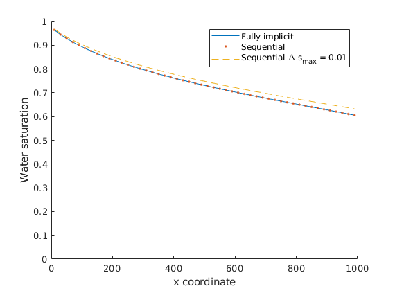
Plot and compare the three different solutions¶

By plotting the three solutions simultanously, we see that the fully implicit and sequential implicit give the same solution for the same timesteps. The solution that is refined in time is quite different, however, demonstrating that the numerical truncation error due to the temporal discretization can significantly impact the simulation results.

x = G.cells.centroids(:, 1);

for i = 1:numel(statesFine)
    figure(1); clf, hold on
    plot(x, states{i}.s(:, 1), '-')
    plot(x, statesSeq{i}.s(:, 1), '.')
    plot(x, statesFine{i}.s(:, 1), '--')
    ylim([0, 1])
    legend('Fully implicit', 'Sequential', 'Sequential \Delta s_{max} = 0.01');
    ylabel('Water saturation');
    xlabel('x coordinate');
    pause(0.1)
end

Copyright notice¶

<html>
% <p><font size="-1

mrstModule add mrst-gui ad-props ad-core ad-blackoil blackoil-sequential msrsb spe10 coarsegrid

Set up simulation problem¶

Generated from relaxedVolumeSPE10.m

totTime = 2000*day;

layers = 5;
nLayers = numel(layers);

% Offsets to move the wells if needed
ofs = [0, 0];
wloc     = [  1 + ofs(1),   60 - ofs(1),     1 + ofs(1),   60 - ofs(1),   30 ;
              1 + ofs(2),    1 + ofs(2),   220 - ofs(2),  220 - ofs(2),  110 ];

[G, W, rock] = getSPE10setup(layers, wloc);

mp = 0.01;
rock.poro(rock.poro < mp) = mp;

pv = poreVolume(G, rock);

% Either two-phase or three-phase
if 1
    compi = [.5, 0, .5];
    sat = [0, 1, 0];
    getmodel = @ThreePhaseBlackOilModel;
else
    compi = [1, 0];
    sat = [0, 1];
    getmodel = @TwoPhaseOilWaterModel;
end

for i = 1:numel(W)
    isinj = W(i).val > 400*barsa;
    if isinj
        W(i).val = sum(pv)/totTime;
        W(i).type = 'rate';
    else
        W(i).val = 4000*psia;
        W(i).type = 'bhp';
    end
    W(i).compi = compi;
    W(i).sign = 1 - 2*~isinj;
end

% Set up model with quadratic relperms and constant compressibility in oil
p0 = 300*barsa;
c = [1e-6, 1e-4, 1e-3]/barsa;
% c = [0,0,0];
fluid = initSimpleADIFluid('mu', [1, 5, 1]*centi*poise, ...
                           'c', c, ...
                           'rho', [1000, 700, 1], 'n', [2 2 2]);

% Fully implicit model
modelfi = getmodel(G, rock, fluid);
% Sequential pressure-transport model with same type


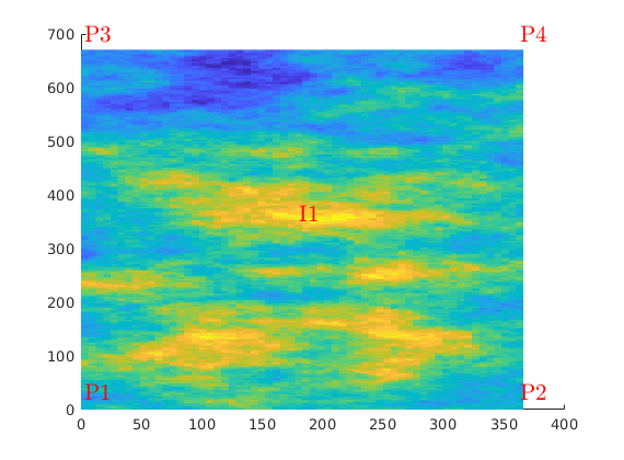
figure;
plotCellData(G, log10(rock.perm(:, 1)), 'edgec', 'none');
plotWell(G, W)
% Set up the schedule
nstep = 100;

dt = rampupTimesteps(totTime, totTime/nstep);
clear schedule;
schedule = simpleSchedule(dt, 'W', W);

state = initResSol(G, p0, sat);

Defaulting reference depth to top of formation for well P1. Please specify 'refDepth' optional argument to 'addWell' if you require bhp at a specific depth.
Defaulting reference depth to top of formation for well P2. Please specify 'refDepth' optional argument to 'addWell' if you require bhp at a specific depth.
Defaulting reference depth to top of formation for well P3. Please specify 'refDepth' optional argument to 'addWell' if you require bhp at a specific depth.
Defaulting reference depth to top of formation for well P4. Please specify 'refDepth' optional argument to 'addWell' if you require bhp at a specific depth.
Defaulting reference depth to top of formation for well I1. Please specify 'refDepth' optional argument to 'addWell' if you require bhp at a specific depth.

Solve a sequential solve¶

We first solve a pressure equation, fix total velocity and solve for n-1 phases. To find the remaining saturation, we use the relation

We naturally incur a bit of mass-balance error for the omitted phase pseudocomponent.

model = getSequentialModelFromFI(modelfi);
model.transportModel.useCNVConvergence = true;

[ws_seq, states_seq, rep_seq] = simulateScheduleAD(state, model, schedule);

*****************************************************************
********** Starting simulation:   108 steps,  2000 days *********
*****************************************************************
Preparing model for simulation...
Model ready for simulation...
Preparing schedule for simulation...
Schedule ready for simulation...
Validating initial state...
...

Solve a second sequential solve¶

We first solve a pressure equation, fix total velocity and solve for all phases/components. We relax the sum of saturations assumption to achieve this.

model.transportModel.conserveOil = true;
model.transportModel.conserveWater = true;
model.transportModel.useCNVConvergence = true;
[ws_seq2, states_seq2, rep_seq2] = simulateScheduleAD(state, model, schedule);

*****************************************************************
********** Starting simulation:   108 steps,  2000 days *********
*****************************************************************
Preparing model for simulation...
Model ready for simulation...
Preparing schedule for simulation...
Schedule ready for simulation...
Validating initial state...
...

Fully-implicit¶

[wsfi, statesfi] = simulateScheduleAD(state, modelfi, schedule);

*****************************************************************
********** Starting simulation:   108 steps,  2000 days *********
*****************************************************************
Preparing model for simulation...
Model ready for simulation...
Preparing schedule for simulation...
Schedule ready for simulation...
Validating initial state...
...

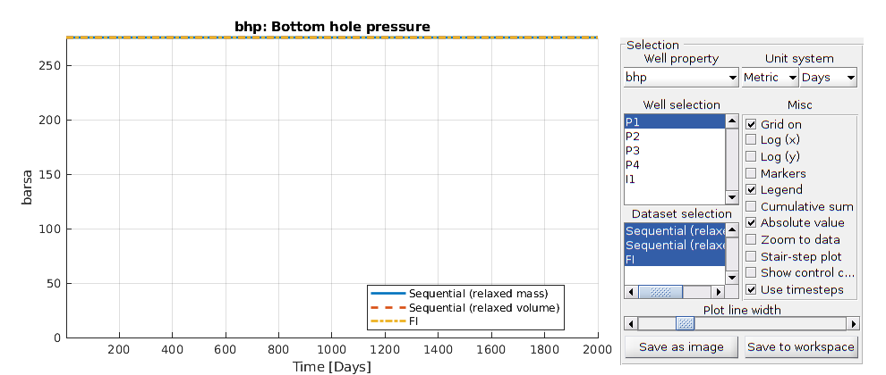
Plot well curves for fully implicit problem¶

plotWellSols({ws_seq, ws_seq2, wsfi}, cumsum(schedule.step.val), 'datasetnames', {'Sequential (relaxed mass)', 'Sequential (relaxed volume)', 'FI'})

Simulate the Egg model¶

Generated from sequentialEGG.m

The Egg model is a nearly incompressible waterflood problem. This example sets up a sequential solver and compares the results with the fully implicit discretization. As there are small changes in mobility, this problem is very well suited to sequential splitting. For details on the EggModel, see Jansen, J. D., et al. “The egg model–a geological ensemble for reservoir simulation.” Geoscience Data Journal 1.2 (2014): 192-195.

mrstModule add ad-core ad-blackoil spe10 blackoil-sequential mrst-gui

% Set up pressure and transport linear solvers
if ~isempty(mrstPath('agmg'))
    mrstModule add agmg
    psolver = AGMGSolverAD();
else
    psolver = BackslashSolverAD();
end
tsolver = GMRES_ILUSolverAD();
% Select layer 1
layers = 1;
mrstModule add ad-core ad-blackoil blackoil-sequential spe10

% The base case for the model is 2000 days. This can be reduced to make the
% problem faster to run.
[G, rock, fluid, deck, state] = setupEGG();
model = selectModelFromDeck(G, rock, fluid, deck);

schedule = convertDeckScheduleToMRST(model, deck);
% Set up the sequential model
seqModel = getSequentialModelFromFI(model, 'pressureLinearSolver', psolver,....
                                           'transportLinearSolver', tsolver);
% Run problem
[wsSeq, statesSeq, repSeq] = simulateScheduleAD(state, seqModel, schedule);

No converter needed in section 'REGIONS'.
No converter needed in section 'SUMMARY'.
Processing Cells     1 : 18553 of 18553 ... done (0.11 [s], 1.65e+05 cells/second)
Total 3D Geometry Processing Time = 0.112 [s]
Ordering well 1 (INJECT1) with strategy "origin".
Ordering well 2 (INJECT2) with strategy "origin".
Ordering well 3 (INJECT3) with strategy "origin".
Ordering well 4 (INJECT4) with strategy "origin".
...

Simulate fully implicit¶

Solve the fully implicit version of the problem, with a CPR preconditioner that uses the same linear solver for the pressure as the sequential solver.

solver = NonLinearSolver();
solver.LinearSolver = CPRSolverAD('ellipticSolver', psolver);

[wsFIMP, statesFIMP, repFIMP] = simulateScheduleAD(state, model, schedule, 'nonlinearsolver', solver);

*****************************************************************
********** Starting simulation:   123 steps,  3600 days *********
*****************************************************************
Preparing model for simulation...
Model ready for simulation...
Preparing schedule for simulation...
Schedule ready for simulation...
Validating initial state...
...

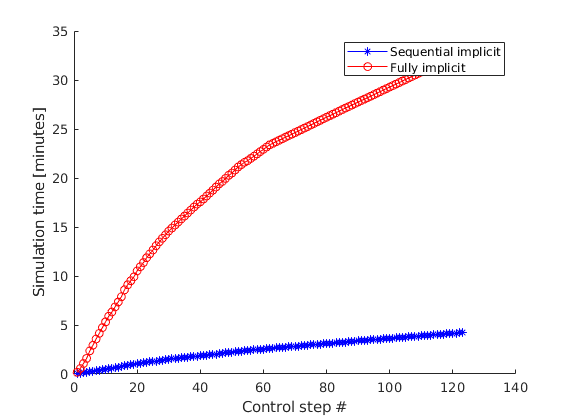
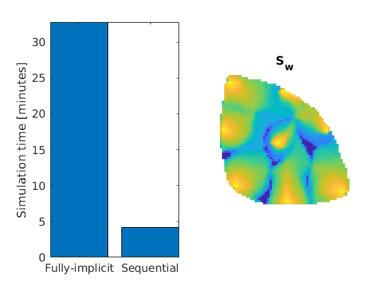
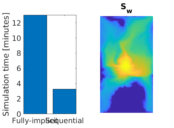
Plot simulation time taken¶

The sequential solver can be much faster than the fully implicit solver for certain problems.

figure(1); clf; hold on
plot(cumsum(repSeq.SimulationTime)/60, 'b-*')
plot(cumsum(repFIMP.SimulationTime)/60, 'r-o')
ylabel('Simulation time [minutes]')
xlabel('Control step #')
legend('Sequential implicit', 'Fully implicit')

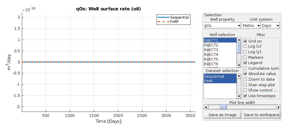
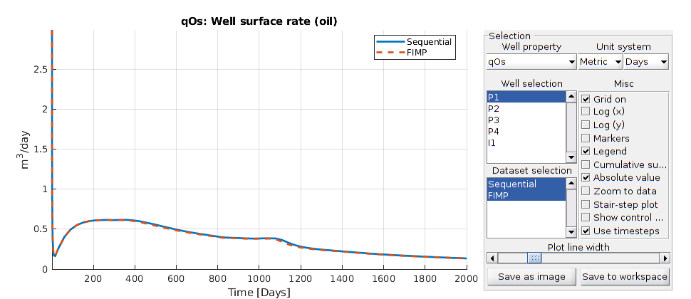
Plot the results in interactive viewers¶

G = model.G;
W = schedule.control(1).W;

% Plot the well curves
plotWellSols({wsSeq, wsFIMP}, cumsum(schedule.step.val), ...
            'datasetnames', {'Sequential', 'FIMP'}, 'field', 'qOs')

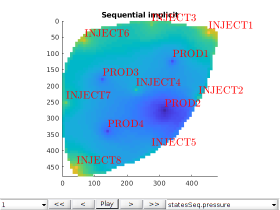
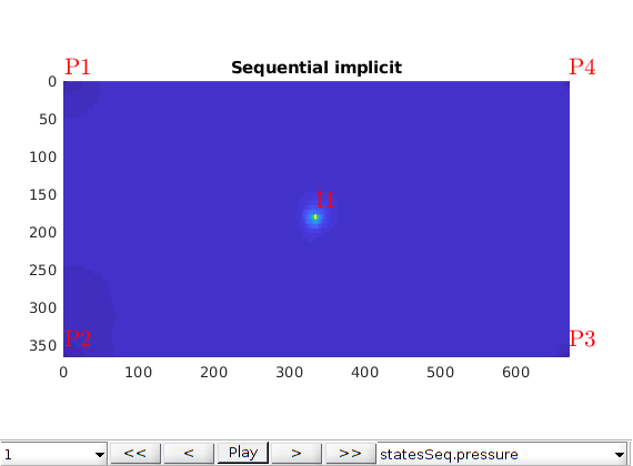
% Plot reservoir quantities
figure;
plotToolbar(G, statesSeq);
axis equal tight
view(90, 90);
plotWell(G, W);
title('Sequential implicit')

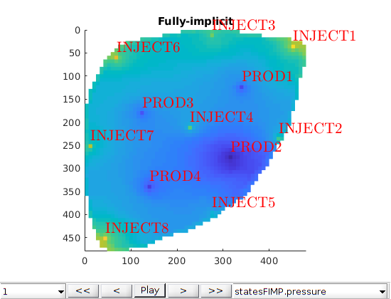
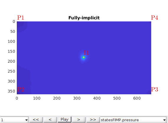
figure;
plotToolbar(G, statesFIMP);
axis equal tight
view(90, 90);
plotWell(G, W);
title('Fully-implicit')

Plot time taken¶

figure;
subplot(1, 2, 1)
bar([sum(repFIMP.SimulationTime), sum(repSeq.SimulationTime)]/60)
set(gca, 'XTickLabel', {'Fully-implicit', 'Sequential'})
ylabel('Simulation time [minutes]')
set(gca, 'FontSize', 12)
axis tight
subplot(1, 2, 2)
plotCellData(model.G, statesSeq{60}.s(:, 1), 'edgecolor', 'none')
title('S_w')
set(gca, 'FontSize', 12)

axis equal tight off

Copyright notice¶

<html>
% <p><font size="-1

Set up and run a five-spot problem with water-alternating-gas (WAG) drive¶

Generated from sequentialFiveSpotWAG.m

One approach to hydrocarbon recovery is to inject gas or water. In the water-alternating-gas approach, wells change between injection of gas and water to improve the sweep efficiency. In this example, we set up a five-spot injection pattern where the injector controls alternate between water and gas. The primary purpose of the example is not to demonstrate an ideal or realistic WAG-configuration, but rather how to set up a problem with changing well controls and to demonstrate how the sequential solvers perform on problems with large changes in mobility and well controls. We begin by loading the required modules

mrstModule add ad-core ad-blackoil ad-props ...
               blackoil-sequential spe10 mrst-gui

Set up grid and rock structure¶

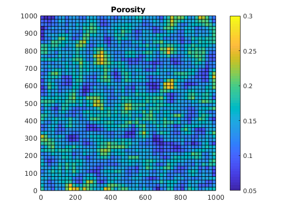
We define a 50x50x1 grid, spanning a 1 km by 1km domain. The porosity is assigned via a Gaussian field and a synthethic permeability is computed using a standard correlation.

cartDims = [50, 50, 1];
physDims = [1000, 1000, 1]*meter;
G = cartGrid(cartDims, physDims);
G = computeGeometry(G);
gravity reset off

rng(0);
poro = gaussianField(cartDims, [0.05, 0.3], 3, 8);
poro = poro(:);
perm = poro.^3 .* (5e-5)^2 ./ (0.81 * 72 * (1 - poro).^2);
% Build rock object
rock = makeRock(G, perm, poro);
figure(1); clf
plotCellData(G, rock.poro)
axis equal tight
colorbar
title('Porosity')

Processing Cells    1 : 2500 of 2500 ... done (0.03 [s], 9.89e+04 cells/second)
Total 3D Geometry Processing Time = 0.025 [s]

Set up wells and schedule¶

The injection scenario corresponds to injecting one pore volume of gas and water over 30 years at standard conditions. We first place wells in the corners of the domain set to fixed injection rates as well as a bottom hole pressure producer in the middle of the domain.

pv = poreVolume(G, rock);
T = 30*year;
irate = sum(pv)/(T*4);
% Function handle for easily creating multiple injectors
makeInj = @(W, name, I, J, compi) verticalWell(W, G, rock, I, J, [],...
    'Name', name, 'radius', 5*inch, 'sign', 1, 'Type', 'rate',...
    'Val', irate, 'comp_i', compi);
W = [];
W = makeInj(W, 'I1', 1,           1,           []);
W = makeInj(W, 'I3', cartDims(1), cartDims(2), []);
W = makeInj(W, 'I4', 1,           cartDims(2), []);
W = makeInj(W, 'I2', cartDims(1), 1,           []);

I = ceil(cartDims(1)/2);
J = ceil(cartDims(2)/2);
% Producer
W = verticalWell(W, G, rock, I, J, [], 'Name', 'P1', 'radius', 5*inch, ...
    'Type', 'bhp', 'Val', 100*barsa, 'comp_i', [1, 1, 1]/3, 'Sign', -1);
% Create two copies of the wells: The first copy is set to water injection
% and the second copy to gas injection.
[W_water, W_gas] = deal(W);
for i = 1:numel(W)
    if W(i).sign < 0
        % Skip producer
        continue
    end
    W_water(i).compi = [1, 0, 0];
    W_gas(i).compi   = [0, 0, 1];
end
% Simulate 90 day time steps, with a gradual increase of steps in the
% beginning as the mobility changes rapidly when wells begin injecting for
% the first time.
dT_target = 90*day;
dt = rampupTimesteps(T, dT_target, 10);

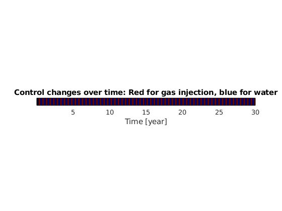
% Set up a schedule with two different controls. In the first control, the
% injectors are set to the copy of the wells we made earlier where water
% was injected. In the second control, gas is injected instead.
schedule = struct();
schedule.control = [struct('W', W_water);...
% Water control 1
                    struct('W', W_gas)]; % Gas control 2
% Set timesteps
schedule.step.val = dt;
% Alternate between the gas and water controls every 90 days
schedule.step.control = (mod(cumsum(dt), 2*dT_target) >= dT_target) + 1;

% Plot the changes in schedule control
figure(1), clf
ctrl = repmat(schedule.step.control', 2, 1);
x = repmat(cumsum(dt/year)', 2, 1);
y = repmat([0; 1], 1, size(ctrl, 2));
surf(x, y, ctrl)
colormap(jet)
view(0, 90)
axis equal tight
set(gca, 'YTick', []);
xlabel('Time [year]')
title('Control changes over time: Red for gas injection, blue for water')

Defaulting reference depth to top of formation for well I1. Please specify 'refDepth' optional argument to 'addWell' if you require bhp at a specific depth.
Defaulting reference depth to top of formation for well I3. Please specify 'refDepth' optional argument to 'addWell' if you require bhp at a specific depth.
Defaulting reference depth to top of formation for well I4. Please specify 'refDepth' optional argument to 'addWell' if you require bhp at a specific depth.
Defaulting reference depth to top of formation for well I2. Please specify 'refDepth' optional argument to 'addWell' if you require bhp at a specific depth.
Defaulting reference depth to top of formation for well P1. Please specify 'refDepth' optional argument to 'addWell' if you require bhp at a specific depth.

Set up fluid and simulation model¶

We set up a three-phase fluid with quadratic relative permeability curves, significant viscosity contrast between the phases and compressibility for the oil and gas phases.

fluid = initSimpleADIFluid('phases',    'WOG', ...
                           'rho',       [1000, 700, 250], ...
                           'n',         [2, 2, 2], ...
                           'c',         [0, 1e-4, 1e-3]/barsa, ...
                           'mu',        [1, 4, 0.25]*centi*poise ...
                           );
% Set up three-phase, immiscible model with fully implicit discretization
model = ThreePhaseBlackOilModel(G, rock, fluid, 'disgas', false, 'vapoil', false);
% Create sequential model from fully implicit model
seqModel = getSequentialModelFromFI(model);
% Set up initial reservoir at 100 bar pressure and completely oil filled.
state = initResSol(G, 100*barsa, [0, 1, 0]);

Simulate the schedule using the sequential solver¶

We simulate the full schedule using simulateScheduleAD

[wsSeq, statesSeq] = simulateScheduleAD(state, seqModel, schedule);

*****************************************************************
********** Starting simulation:   132 steps, 10950 days *********
*****************************************************************
Preparing model for simulation...
Model ready for simulation...
Preparing schedule for simulation...
Schedule ready for simulation...
Validating initial state...
...

Simulate the schedule using a fully implicit solver¶

For comparison purposes, we also solve the fully implicit case

[wsFIMP, statesFIMP] = simulateScheduleAD(state, model, schedule);

*****************************************************************
********** Starting simulation:   132 steps, 10950 days *********
*****************************************************************
Preparing model for simulation...
Model ready for simulation...
Preparing schedule for simulation...
Schedule ready for simulation...
Validating initial state...
...

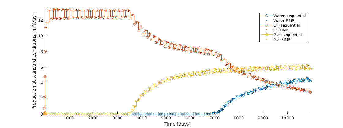
Plot producer rates¶

We plot the producer water, gas and oil rates. We can see the effect of the alternating controls directly on the production curves and we use a stairstep plot since the underlying data is not continuous.

df = get(0, 'DefaultFigurePosition');
figure('position', df.*[1, 1, 2, 1])
names = {'qWs', 'qOs', 'qGs'};
hold on
t = cumsum(schedule.step.val)/day;
colors = lines(3);

% q = getWellOutput(wsSeq, 'qWs'
for i = 1:numel(names)
%     subplot(1, 3, 1)
    qSeq = -getWellOutput(wsSeq, names{i}, 5);
    qFIMP = -getWellOutput(wsFIMP, names{i}, 5);
    stairs(t, qSeq*day, '-o', 'color', colors(i, :));
    stairs(t, qFIMP*day, '.', 'color', colors(i, :), 'linewidth', 2);
end
legend('Water, sequential', 'Water FIMP', 'Oil, sequential', ...
       'Oil FIMP', 'Gas, sequential', 'Gas FIMP');
xlabel('Time [days]')
ylabel('Production at standard conditions [m^3/day]')
axis tight

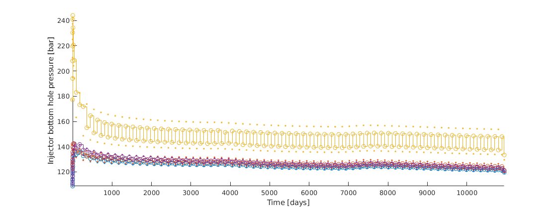
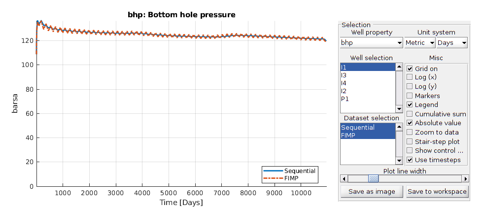
Plot the injector bottom hole pressure¶

The injector bottom hole pressure has a bigger discrepancy between the two schemes, since the injectors use the cell total mobility to compute the relation between completion flux and bottom hole pressure. The deviation between the schemes is a direct result of the lagging mobility values in the pressure equation.

clf; hold on
colors = lines(4);

for i = 1:4
    bhpSeq = getWellOutput(wsSeq, 'bhp', i)/barsa;
    bhpFIMP = getWellOutput(wsFIMP, 'bhp', i)/barsa;

    stairs(t, bhpSeq, '-o', 'color', colors(i, :));
    stairs(t, bhpFIMP, '.', 'color', colors(i, :), 'linewidth', 2);
end
xlabel('Time [days]')
ylabel('Injector bottom hole pressure [bar]')
axis tight

Launch interactive plotting¶

Finally we launch interactive viewers for the well curves and reservoir quantities.

plotWellSols({wsSeq, wsFIMP}, cumsum(schedule.step.val), ...
    'datasetnames', {'Sequential', 'FIMP'}, 'linestyles', {'-', '-.'})

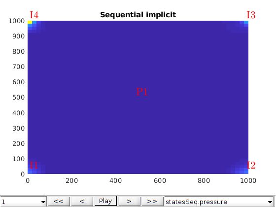
figure;
plotToolbar(G, statesSeq);
axis tight
plotWell(G, W);
title('Sequential implicit')

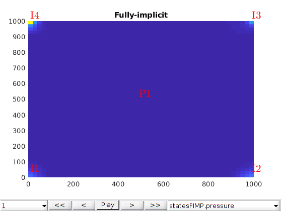
figure;
plotToolbar(G, statesFIMP);
axis tight
plotWell(G, W);
title('Fully-implicit')

Copyright notice¶

<html>
% <p><font size="-1

Compare sequential solver to fully implicit, applied to the SPE1 problem¶

Generated from sequentialSPE1.m

This example simulates the first SPE benchmark using both sequential and fully implicit solvers. The problem is a gas injection with significant density and mobility changes between phases, so the assumption of a constant total velocity for the sequential scheme is violated, and there are differences in production profiles between the two schemes. We also test a third approach, wherein the sequential scheme revisits the pressure solution if the mobilities change significantly, in order to convergence to the fully implicit solution.

mrstModule add ad-core ad-blackoil ad-props

Set up the initial simulation model¶

We use the existing setupSPE1 routine to handle the setup of all parameters, which are then converted into a fully implicit model and a schedule.

[G, rock, fluid, deck, state] = setupSPE1();

model = selectModelFromDeck(G, rock, fluid, deck);
schedule = convertDeckScheduleToMRST(model, deck);

No converter needed in section 'REGIONS'.
No converter needed in section 'SUMMARY'.
Adding 200 artificial cells at top/bottom

Processing regular i-faces
 Found 550 new regular faces
Elapsed time is 0.006272 seconds.

...

Run the entire fully implicit schedule¶

We simulate the schedule with a fully implicit scheme, i.e. where we solve for both saturations and pressure simultanously.

[wsFIMP, statesFIMP, repFIMP] = simulateScheduleAD(state, model, schedule);

*****************************************************************
********** Starting simulation:   120 steps,  1216 days *********
*****************************************************************
Preparing model for simulation...
Model ready for simulation...
Preparing schedule for simulation...
Schedule ready for simulation...
Validating initial state...
...

Set up and simulate the schedule using a sequential implicit scheme¶

We convert the fully implicit model into a sequential model, a special model which contains submodels for both the pressure and transport. In this scheme, we first solve the pressure equation implicitly to obtain total volumetric fluxes at reservoir conditions, as well as total well rates. The pressure and fluxes are subsequently used as input for the transport scheme, which advects the saturations in the total velocity field using a fractional flow formulation.

seqModel = getSequentialModelFromFI(model);
[wsSeq, statesSeq, repSeq] = simulateScheduleAD(state, seqModel, schedule);

*****************************************************************
********** Starting simulation:   120 steps,  1216 days *********
*****************************************************************
Preparing model for simulation...
Model ready for simulation...
Preparing schedule for simulation...
Schedule ready for simulation...
Validating initial state...
...

Simulate the schedule with the outer loop option enabled¶

In the sequential implicit scheme, the transport equations are derived by assuming a fixed total velocity. For certain problems, this assumption is not reasonable, and the total velocity may be strongly coupled to the changes in saturation during a timestep. In this case, the problem is a gas injection scenario where the injected gas has a much higher mobility and much lower density, leading to significantly different results between the fully implicit and the sequential implicit schemes. One way to improve the results of the sequential implicit scheme is to employ an outer loop when needed. This amounts to revisiting the pressure equation after the transport has converged and checking if the pressure equation is still converged after the saturations have changed. If the pressure equation has a large residual after the transport, we then resolve the pressure with the new estimates for saturations.

% Make a copy of the model
seqModelOuter = seqModel;
% Disable the "stepFunctionIsLinear" option, which tells the
% NonLinearSolver that it is not sufficient to do a single pressure,
% transport step to obtain convergence. We set ds tolerance to 0.001
% (which is also the default) which is roughly equivalent to the maximum
% saturation error convergence criterion used in the fully implicit solver.
seqModelOuter.stepFunctionIsLinear = false;
seqModelOuter.incTolSaturation = 1.0000e-03;


[wsOuter, statesOuter, repOuter] = simulateScheduleAD(state, seqModelOuter, schedule);

*****************************************************************
********** Starting simulation:   120 steps,  1216 days *********
*****************************************************************
Preparing model for simulation...
Model ready for simulation...
Preparing schedule for simulation...
Schedule ready for simulation...
Validating initial state...
...

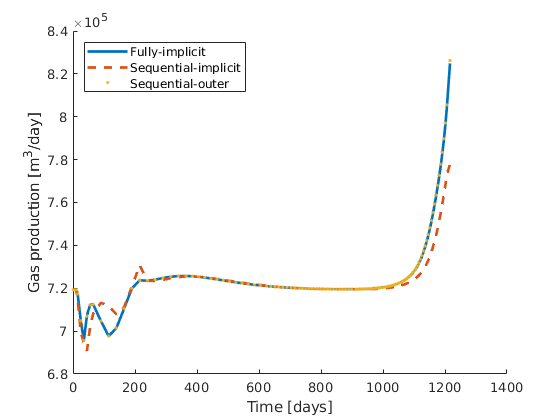
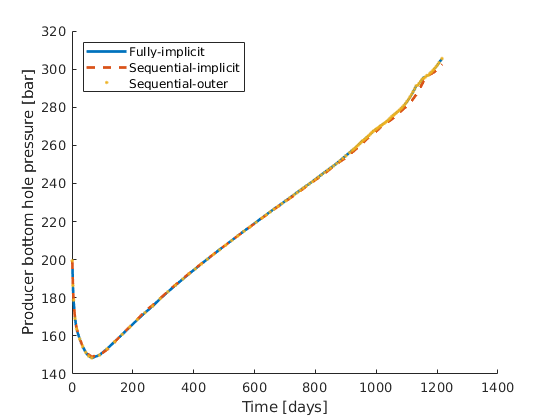
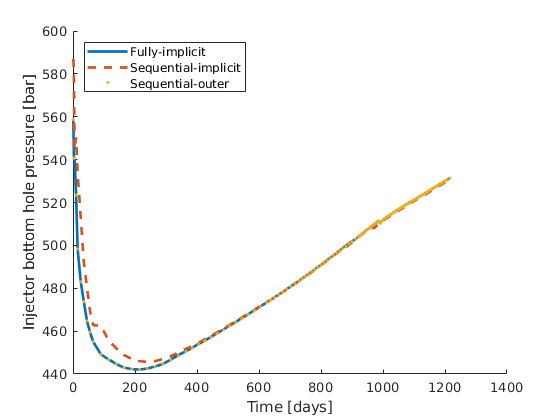
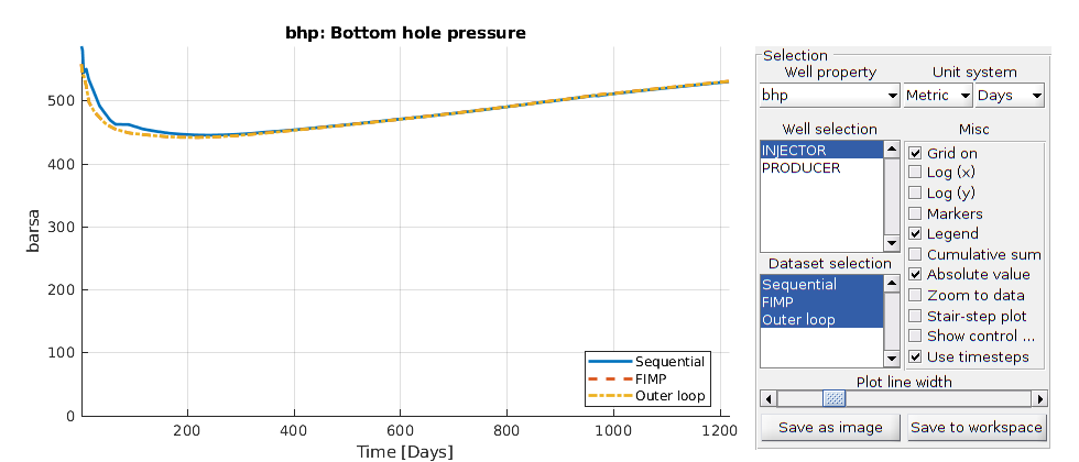
Plot the results¶

We plot the results for the three different temporal discretization schemes. Since the water is close to immobile and the injector and producers are operated on gas and oil rates respectively, we plot the gas production and the bottom hole pressure for each well. We clearly see that there are substantial differences in the well curves due the changes in total velocity. The sequential implicit scheme with the outer loop enabled is very close to the fully implicit solution and will get closer if the tolerances are tightened.

T = cumsum(schedule.step.val);

wellSols = {wsFIMP, wsSeq, wsOuter};
states = {statesFIMP, statesSeq, statesOuter};
names = {'Fully-implicit', 'Sequential-implicit', 'Sequential-outer'};
markers = {'-', '--', '.'};

close all;
for i = 1:numel(wellSols)
    figure(1); hold on
    qo = -getWellOutput(wellSols{i}, 'qGs', 2)*day;
    plot(T/day, qo, markers{i}, 'linewidth', 2)
    xlabel('Time [days]');
    ylabel('Gas production [m^3/day]');

    figure(2); hold on
    bhp = getWellOutput(wellSols{i}, 'bhp', 2)/barsa;
    plot(T/day, bhp, markers{i}, 'linewidth', 2)
    xlabel('Time [days]');
    ylabel('Producer bottom hole pressure [bar]');

    figure(3); hold on
    bhp = getWellOutput(wellSols{i}, 'bhp', 1)/barsa;
    plot(T/day, bhp, markers{i}, 'linewidth', 2)
    xlabel('Time [days]');
    ylabel('Injector bottom hole pressure [bar]');
end

% Add legends to the plots
for i = 1:3
    figure(i);
    legend(names, 'location', 'northwest')
end

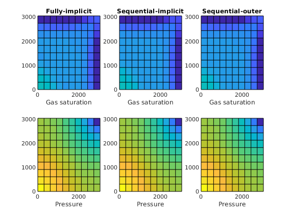
% Plot the different saturations and pressures
figure;
for i = 1:numel(names)
    s = states{i};

    subplot(2, numel(names), i)
    plotCellData(model.G, s{end}.s(:, 3))
    caxis([0, 1])
    axis tight
    title(names{i})
    xlabel('Gas saturation')

    subplot(2, numel(names), i + numel(names))
    plotCellData(model.G, s{end}.pressure)
    axis tight
    xlabel('Pressure')
end

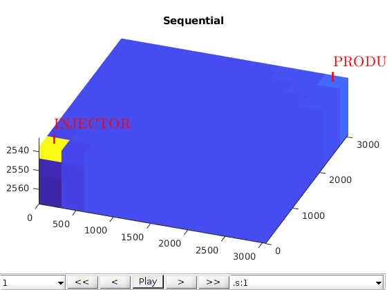
Set up interactive plotting¶

We finish the example by launching interactive viewers for the well curves, as well as the different reservoir quantities.

mrstModule add mrst-gui
wsol = {wsSeq, wsFIMP, wsOuter};
wnames = {'Sequential', 'FIMP', 'Outer loop'};
states = {statesSeq, statesFIMP, statesOuter};

for i = 1:numel(states)
    figure(i), clf
    plotToolbar(G, states{i});
    title(wnames{i});
    axis tight
    view(20, 60);
    plotWell(G, schedule.control(1).W)
end

plotWellSols(wsol, T, 'datasetnames', wnames)

Copyright notice¶

<html>
% <p><font size="-1

Solve layers of SPE10 with sequential and fully implicit solver¶

Generated from sequentialSPE10.m

This is a short example demonstrating how to solve any number of layers of the SPE10, model 2 problem using both a sequential and a fully implicit solver.

mrstModule add ad-core ad-blackoil spe10 blackoil-sequential mrst-gui

% Set up pressure and transport linear solvers
if ~isempty(mrstPath('agmg'))
    mrstModule add agmg
    psolver = AGMGSolverAD();
else
    psolver = BackslashSolverAD();
end
tsolver = GMRES_ILUSolverAD();
% Select layer 1
layers = 1;
mrstModule add ad-core ad-blackoil blackoil-sequential spe10

% The base case for the model is 2000 days. This can be reduced to make the
% problem faster to run.
T = 2000*day;
[state, model, schedule] = setupSPE10_AD('layers', layers, 'dt', 30*day, ...
                                                           'T',  T);
% Set up the sequential model
seqModel = getSequentialModelFromFI(model, 'pressureLinearSolver', psolver,....
                                           'transportLinearSolver', tsolver);
% We set up a timestep selector that aims for timesteps where the
% maximum saturation change is equal to a fixed value.
stepSel = StateChangeTimeStepSelector('targetProps', {'s'},...
                                      'targetChangeAbs', 0.25);
% Run problem
solver = NonLinearSolver('timeStepSelector', stepSel);
[wsSeq, statesSeq, repSeq] = simulateScheduleAD(state, seqModel, schedule, 'NonLinearSolver', solver);

Defaulting reference depth to top of formation for well P1. Please specify 'refDepth' optional argument to 'addWell' if you require bhp at a specific depth.
Defaulting reference depth to top of formation for well P2. Please specify 'refDepth' optional argument to 'addWell' if you require bhp at a specific depth.
Defaulting reference depth to top of formation for well P3. Please specify 'refDepth' optional argument to 'addWell' if you require bhp at a specific depth.
Defaulting reference depth to top of formation for well P4. Please specify 'refDepth' optional argument to 'addWell' if you require bhp at a specific depth.
Defaulting reference depth to top of formation for well I1. Please specify 'refDepth' optional argument to 'addWell' if you require bhp at a specific depth.
*****************************************************************
********** Starting simulation:    75 steps,  2000 days *********
*****************************************************************
...

Simulate fully implicit¶

Solve the fully implicit version of the problem, with a CPR preconditioner that uses the same linear solver for the pressure as the sequential solver.

solver.timeStepSelector.reset();
solver.LinearSolver = CPRSolverAD('ellipticSolver', psolver);

[wsFIMP, statesFIMP, repFIMP] = simulateScheduleAD(state, model, schedule, 'NonLinearSolver', solver);

*****************************************************************
********** Starting simulation:    75 steps,  2000 days *********
*****************************************************************
Preparing model for simulation...
Model ready for simulation...
Preparing schedule for simulation...
Schedule ready for simulation...
Validating initial state...
...

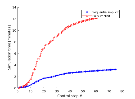
Plot simulation time taken¶

The sequential solver can be much faster than the fully implicit solver for certain problems.

figure(1); clf; hold on
plot(cumsum(repSeq.SimulationTime)/60, 'b-*')
plot(cumsum(repFIMP.SimulationTime)/60, 'r-o')
ylabel('Simulation time [minutes]')
xlabel('Control step #')
legend('Sequential implicit', 'Fully implicit')

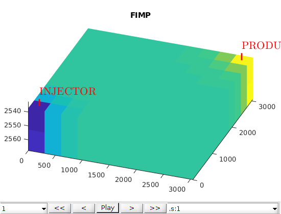
Plot the results in interactive viewers¶

G = model.G;
W = schedule.control(1).W;

% Plot the well curves
plotWellSols({wsSeq, wsFIMP}, cumsum(schedule.step.val), ...
            'datasetnames', {'Sequential', 'FIMP'}, 'field', 'qOs')

% Plot reservoir quantities
figure;
plotToolbar(G, statesSeq);
axis equal tight
view(90, 90);
plotWell(G, W);
title('Sequential implicit')

figure;
plotToolbar(G, statesFIMP);
axis equal tight
view(90, 90);
plotWell(G, W);
title('Fully-implicit')

figure;
subplot(1, 2, 1)
bar([sum(repFIMP.SimulationTime), sum(repSeq.SimulationTime)]/60)
set(gca, 'XTickLabel', {'Fully-implicit', 'Sequential'})
ylabel('Simulation time [minutes]')
set(gca, 'FontSize', 18)
axis tight
subplot(1, 2, 2)
plotCellData(model.G, statesSeq{60}.s(:, 1), 'edgecolor', 'none')
title('S_w')
set(gca, 'FontSize', 18)

axis equal tight off

Copyright notice¶

<html>
% <p><font size="-1

blackoil-sequential: Sequential implicit black-oil solvers¶

Models¶

Base classes¶

Utilities¶

Examples¶

Buckley-Leverett problem with multiple substeps¶

Set up model¶

Solve fully implicit base case¶

Get a sequential model¶

Simulate sequential base case¶

Set up timestep selection based on target change quantities¶

Simulate with refined timesteps¶

Plot and compare the three different solutions¶

Copyright notice¶

Set up simulation problem¶

Solve a sequential solve¶

Solve a second sequential solve¶

Fully-implicit¶

Plot well curves for fully implicit problem¶

Simulate the Egg model¶

Simulate fully implicit¶

Plot simulation time taken¶

Plot the results in interactive viewers¶

Plot time taken¶

Copyright notice¶

Set up and run a five-spot problem with water-alternating-gas (WAG) drive¶

Set up grid and rock structure¶

Set up wells and schedule¶

Set up fluid and simulation model¶

Simulate the schedule using the sequential solver¶

Simulate the schedule using a fully implicit solver¶

Plot producer rates¶

Plot the injector bottom hole pressure¶

Launch interactive plotting¶

Copyright notice¶

Compare sequential solver to fully implicit, applied to the SPE1 problem¶

Set up the initial simulation model¶

Run the entire fully implicit schedule¶

Set up and simulate the schedule using a sequential implicit scheme¶

Simulate the schedule with the outer loop option enabled¶

Plot the results¶

Set up interactive plotting¶

Copyright notice¶

Solve layers of SPE10 with sequential and fully implicit solver¶

Simulate fully implicit¶

Plot simulation time taken¶

Plot the results in interactive viewers¶

Copyright notice¶

`blackoil-sequential`: Sequential implicit black-oil solvers¶