`dfm`: Discrete fracture matrix implementation¶

This is the Discrete Fracture Matrix module developed as an extension of MRST.

The module is devopled at the University of Bergen, and licenced under the GNU General Public License v3.0.

The module is mainly developed by Tor Harald Sandve (at IRIS from Jan 2013), minor modifications are introduced by Eirik Keilegavlen (UoB). Some utility files are partly written at Uni Research.

An overview of the files can be found in Content.m

To get started, see the examples subdirectory.

The performance of the hybrid discretization is described in: Sandve, T. H., I. Berre, J. M. Nordbotten (2012), An efficient Multi-Point Flux Approximation based approach for Discrete Fracture Matrix simulation, Journal of Computational Physics, 231(9), 3784-3800, doi:10.1016/j.jcp.2012.01.023.

Some thoughts on the implementation, and more general on discretization on fractured media can be found in Implementation_Notes.pdf

Contents¶

Discrete Fracture Matrix (DFM) module

Routines supporting the DFM method. Examples in /examples Add module by typing MrstModule add dfm AUTHOR: tor.harald.sandve@iris.no

new files

addhybrid - Add hybrid cells to the grid structure. build_fractures_mod - Build fracture network that serves as constraints in the triangulation. computeHybridTrans - Computes the hybrid-hybrid transmissibilities between a hybrid cell 1 and 2 nodeType - return node type plotEdges - plot lines testNormals - Tests if the normals points from neighbor 1 to 2 and returns the index of triangulate - Make a Delaunay Triangulation and return a Mrst grid

/plotting/plotFractures - Plots 2d hybridcells.

Files modified from core MRST functions. Use these to

computeTrans_DFM - Compute transmissibilities using a two-point scheme. computeMultiPointTrans_DFM - Compute multi-point transmissibilities. twophaseJacobian_DFM - Residual and Jacobian of single point upwind solver for two-phase flow. explicitTransport_DFM - Explicit single point upwind transport solver for two-phase flow. implicitTransport_DFM - Implicit single point upwind transport solver for two-phase flow. removeInternalBoundary_DFM - Remove internal boundary in grid by merging faces in face list N

/plotting/ - Modification to plotting rutines to handle

/private.

Files needed since we can not access private folders from this location

/examples:

add_point - Add a new point to the cloud. computeHybridMPTrans - Computes the hybrid-hybrid transmissibilities. Also update the grid and computeTimeOfFlight_DFM - Compute time of flight using finite-volume scheme. distance_to_closest_line - Copyright 2011-2012 University of Bergen incompMPFA_DFM - Solve incompressible flow problem (fluxes/pressures) using MPFA-O method. incompTPFA_DFM - Solve incompressible flow problem (fluxes/pressures) using TPFA method. lines_intersect - [pt] = lines_intersect (vertices, edge1, edge2) partition_edges - [vertices, new_edges, num_added] = … read_openoffice - Read fractures drawn in Libreoffice, and represent them as points and removeFractureIntersections - Partition intersecting edges by adding a point in the intersection. remove_closepoints - Remove all points that are too close to the lines, since these will only snap_to_grid - Move vertices to the closest (structured) grid point. split_edge - Split an edge into two parts

add_point(vertices, pt, box, opts)¶

Add a new point to the cloud.

Ensure the existence of a point in the vertex set if it is not already there. When the function return, the point will be present at vertices(i). new_point contains 0 if an old point was found, and 1 if a new point is created, i.e. it is the number of points added.

addhybrid(G, hybrids, apertures, varargin)¶

Add hybrid cells to the grid structure.

A hybrid cell can be considered a lower-dimensional object in the geometrical grid, that still has a volume in the computational grid. Hybrid cells are created by converting a face into a thin cell. The hybrid cell consist of the same number of points as the corresponding face, but a volume = aperture * A associated with each of the hybrid cell, where A is the hybrid face area.

In addition to the original faces (the ones that the hybrid cell was created from) the hybrid cells consists of hybrid faces. They are lines in 3d and points in 2d, but with an area = aperture * L (3d) and area = aperture (2d), where L is the length of the corresponding face edge.

The hybrid cells will be connected both to ‘normal’ cells (the ones that used to share a face before the the hybrid cells was squeezed in) and possibly other hybrid cells (if the face formed a segment of a longer fracture, say). The former connections are stored in G.faces.neighbors, for details on the ordering of faces etc see comments within the subfunction ‘createHybridCells’ below. Connections between hybrid neighbors are stored in a special field G.hybridNeighbors. For flow calculations on the resulting grid hybrid transmissibilities between the hybrid faces can be computed from computeHybridTrans.m or computeHybridMPTrans.m

If fractures (e.g. lines / planes of multiple hybrid cells) intersects, a small cell may be created in the intersection. However, this has a really small volume, and it may be desirable to eliminate it in flow calculations. This is done by default, unless the optional field addHybrid2Cells is set to true. The elimination results in non-neighbor cell-to-cell connections between hybrid cells that are stored in G.hybridNeighbors.

SYNOPSIS

G = addhybrid(G,faces,apertures)

Parameters:	G – Grid data structure. faces – Logical Vector of face indices. A hybrid cell is created for each true face. apertures – Vector of size G.faces.num giving the aperture of the hybrid cell.

OPTIONS:

addHybrid2Cells - adds hybrids cells of second kind (explanation above): and remove the internal boundary between the rest of the hybrid faces i.e no cell2cell connection are needed.
addCorners - hybrid cells of second kind are created: in the corners

EX:

Create a standard grid: G = tensorGrid(linspace(0,10,11),linspace(0,10,11)); G = computeGeometry(G);
Create a fracture at y=5: hit=find(G.faces.centroids(:,2)==5);
Mark the face as a fracture face: G.faces.tags=zeros(G.faces.num,1); G.faces.tags(hit)=1;
Assign aperture: apt = zeros(G.faces.num,1); apt(hit) = 0.001;
Add the hybrid cells: G = addhybrid(G,G.faces.tags > 0,apt);
Plot the grid: plotGrid(G); plotFractures(G);

This file is licensed under the GNU General Public License v3.0.

build_fractures_mod(opts)¶

Build fracture network that serves as constraints in the triangulation.

Currently only odp-files are read, but other user-specified formats can easily be added here.

computeHybridMPTrans(g, S)¶

Computes the hybrid-hybrid transmissibilities. Also update the grid and

transmissibility structure accordingly.

The call to computeMultiPointTrans with hybrid = true gives a transmissibility matrix where connections between hybrid cells are represented as boundaries (they are not connectiod). This function modifies the transmissibility matrix to produce connected faces. In the case that more than two hybrid cells meets (fracture intersection), we furthermore remove the small cell in the interaction.

If the pressure values at the intersections between hybrid cells are denoted u_0, the discretized elliptic pressure equation can be splitt such that:

( A B^T ; B D ) (u u0)^T = (f 0)^T,

The pressure at the intersection can then be removed such that

u0 = inv(D)*B

Using the above expression the flux can be expressed% q = (T T0) (u u0)^T = (T - T0*inv(D)*B)u

SYNOPSIS

[g, S] = computeHybridMPTrans(g,S)

PARAMETERS

g - Grid data structure. S - Transmissibility data structure.

Copyright 2011-2012 University of Bergen

This file is licensed under the GNU General Public License v3.0.

computeHybridTrans(G, T)¶

Computes the hybrid-hybrid transmissibilities between a hybrid cell 1 and 2 using the star-delta transformation:

t_12 = t_1*t_2/sum(t_k)

for all cells k connected to an intersection.

SYNOPSIS

[G, ft_hybrid] = computeHybridTrans(G,T)

Parameters:	G – Grid data structure. T – Half-Transmissibilities one for each cell face.
Returns:	G – Grid structure with cell-to-cell connections added ft_hybrid – Transmissibilities for each hybrid cell2cell connection.

This file is licensed under the GNU General Public License v3.0.

computeMultiPointTrans_DFM(g, rock, varargin)¶

Compute multi-point transmissibilities.

Synopsis:

T = computeMultiPointTrans_DFM(G, rock)

Parameters:

G – Grid data structure as described by grid_structure.
rock –
Rock data structure with valid field ‘perm’. The permeability is assumed to be in measured in units of metres squared (m^2). Use function ‘darcy’ to convert from (milli)darcies to m^2, e.g.,

perm = convertFrom(perm, milli*darcy)

if the permeability is provided in units of millidarcies.

The field rock.perm may have ONE column for a scalar permeability in each cell, TWO/THREE columns for a diagonal permeability in each cell (in 2/3 D) and THREE/SIX columns for a symmetric full tensor permeability. In the latter case, each cell gets the permeability tensor

K_i = [ k1 k2 ] in two space dimensions

[ k2 k3 ]

K_i = [ k1 k2 k3 ] in three space dimensions

[ k2 k4 k5 ] [ k3 k5 k6 ]

OPTIONAL PARAMETERS

verbose - Whether or not to emit informational messages throughout the: computational process. Default value depending on the settings of function ‘mrstVerbose’.

facetrans -

hybrid - If true, the interaction region is splitted for all nodes: shared by more then one hybrid cell. And the continuity point is moved half an aperture in the normal direction.

Returns:	T – half-transmissibilities for each local face of each grid cell in the grid. The number of half-transmissibilities equal the number of rows in G.cells.faces.

COMMENTS:: PLEASE NOTE: Face normals have length equal to face areas.

See also

incompMPFA, mrstVerbose.

computeTimeOfFlight_DFM(state, G, rock, varargin)¶

Compute time of flight using finite-volume scheme.

MODIFIED FROM computeTimeOfFlight.m to allow for cell 2 cell connections: Copyright (C) in portion 2013 IRIS AS

Synopsis:

 T        = computeTimeOfFlight(state, G, rock)
 T        = computeTimeOfFlight(state, G, rock, 'pn1', pv1, ...)

[T, A]    = computeTimeOfFlight(...)
[T, A, q] = computeTimeOfFlight(...)

Description:

Compute time of flight by solving

nabla·(vT) = phi

using a first-order finite-volume method with upwind flux.

Keyword Arguments:
Parameters:	G – Grid structure. rock – Rock data structure. Must contain a valid porosity field, ‘rock.poro’. state – Reservoir and well solution structure either properly initialized from functions ‘initResSol’ and ‘initWellSol’ respectively, or the results from a call to function ‘solveIncompFlow’. Must contain valid cell interface fluxes, ‘state.flux’.
	wells – Well structure as defined by function ‘addWell’. May be empty (i.e., wells = []) which is interpreted as a model without any wells. src – Explicit source contributions as defined by function ‘addSource’. May be empty (i.e., src = []) which is interpreted as a reservoir model without explicit sources. bc – Boundary condition structure as defined by function ‘addBC’. This structure accounts for all external boundary conditions to the reservoir flow. May be empty (i.e., bc = []) which is interpreted as all external no-flow (homogeneous Neumann) conditions. ‘reverse’ – Reverse the fluxes and rates. ‘tracer’ – Cell-array of cell-index vectors for which to solve tracer equation. One equation is solved for each vector with tracer injected in cells given indices. Each vector adds one additional RHS to the original tof-system. Output given as additional columns in T.
Returns:	T – Cell values of a piecewise constant approximation to time-of-flight computed as the solution of the boundary-value problem () nabla·(vT) = phi using a finite-volume scheme with single-point upwind approximation to the flux. A – Discrete left-hand side of (), a G.cells.num-by-G.cells.num matrix whose entries are A_ij = min(F_ij, 0), and A_ii = sum_j max(F_ij, 0) + max(q_i, 0), where F_ij = -F_ji is the flux from cell i to cell j F_ij = A_ij·n_ij·v_ij. and n_ij is the outward-pointing normal of cell i for grid face ij. OPTIONAL. Only returned if specifically requested. q – Aggregate source term contributions (per grid cell) from wells, explicit sources and boundary conditions. These are the contributions referred to as ‘q_i’ in the definition of the matrix elements, ‘A_ii’. Measured in units of m^3/s. OPTIONAL. Only returned if specifically requested.

See also

simpleTimeOfFlight, solveIncompFlow.

computeTrans_DFM(G, rock, varargin)¶

Compute transmissibilities using a two-point scheme.

Synopsis:

T = computeTrans_DFM(G, rock)
T = computeTrans_DFM(G, rock, 'pn', pv, ...)

This function is modified from the original computeTrans to include hybrid (essentially lower-dimensional) cells representing fractures etc. The hybrid cells are located on the interface between two ‘normal’ cells and have no extension (they are lines in 2D and planes in 3D) in the geometric grid. However, they are accounted for in the computational grid and are assigned an area (2D) or volume (3D). For more information see Karimi-Fard (SPE 2004).

This function is a part of the DFM-module of MRST, and should be applied together with other functions of that module.

Keyword Arguments:
Parameters:	G – Grid structure as described by grid_structure. rock – Rock data structure with valid field ‘perm’. The permeability is assumed to be in measured in units of meters squared (m^2). Use function ‘darcy’ to convert from darcies to m^2, e.g., perm = convertFrom(perm, milli*darcy) if the permeability is provided in units of millidarcies. The field rock.perm may have ONE column for a scalar permeability in each cell, TWO/THREE columns for a diagonal permeability in each cell (in 2/3 D) and THREE/SIX columns for a symmetric full tensor permeability. In the latter case, each cell gets the permeability tensor K_i = [ k1 k2 ] in two space dimensions [ k2 k3 ] K_i = [ k1 k2 k3 ] in three space dimensions [ k2 k4 k5 ] [ k3 k5 k6 ]
	K_system – Define the system permeability is defined in valid values are ‘xyz’ and ‘loc_xyz’. cellCenters – Compute transmissibilities based on supplied cellCenters rather than default G.cells.centroids cellFaceCenters – Compute transmissibilities based on supplied cellFaceCenters rather then default G.faces.centroids(G.cells.faces(:,1), :) hybrid – if true the distance between the cell center and the face center is extended half an aperture in the direction of the normal. compactNeighboringCell – Whether hybrid faces should be expanded for the cells on both sides of the face. Only activated if hybrid is true
Returns:	T – half-transmissibilities for each local face of each grid cell in the grid. The number of half-transmissibilities equals the number of rows in G.cells.faces.

COMMENTS:: PLEASE NOTE: Face normals are assumed to have length equal to the corresponding face areas. This property is guaranteed by function ‘computeGeometry’.

distance_to_closest_line(varargin)¶

This file is licensed under the GNU General Public License v3.0.

explicitTransport_DFM(state, G, tf, rock, fluid, varargin)¶

Explicit single point upwind transport solver for two-phase flow.

Synopsis:

state = explicitTransport_DFM(state, G, tf, rock, fluid)
state = explicitTransport_DFM(state, G, tf, rock, fluid, 'pn1', pv1, ...)

Description:

Function explicitTransport solves the Buckley-Leverett transport equation

s_t + /· [f(s)(v·n + mo(rho_w - rho_o)n·Kg)] = f(s)q

using a first-order mobility-weighted upwind discretisation in space and a forward Euler discretisation in time. The transport equation is solved on the time interval [0,tf] by calling twophaseJacobian to build a function computing the residual of the discrete system in addition to a function taking care of the update of the solution during the time loop.

This file is modified from the original explicit transport method to account for hybrid (fracture) cells.

Keyword Arguments:
Parameters:	state – Reservoir and well solution structure either properly initialized from functions ‘initResSol’ and ‘initWellSol’ respectively, or the results from a previous call to function ‘solveIncompFlow’ and, possibly, a transport solver such as function ‘implicitTransport’. G – Grid data structure discretising the reservoir model. tf – End point of time integration interval (i.e., final time). Measured in units of seconds. rock – Rock data structure. Must contain the field ‘rock.poro’, and in the presence of gravity, valid permeabilities measured in units of m^2 in field ‘rock.perm’. fluid – Fluid data structure as defined in ‘fluid_structure’.
	wells – Well structure as defined by function ‘addWell’. This structure accounts for all injection and production well contribution to the reservoir flow. Default value: wells = [], meaning a model without any wells. bc – Boundary condtion structure as defined by function ‘addBC’. This structure accounts for all external boundary contributions to the reservoir flow. Default value: bc = [] meaning all external no-flow (homogeneous Neumann) conditions. src – Explicit source contributions as defined by function ‘addSource’. Default value: src = [] meaning no explicit sources exist in the model. onlygrav – Ignore content of state.flux. Default false. computedt – Estimate time step. Default true. max_dt – If ‘computedt’, limit time step. Default inf. dt_factor – Safety factor in time step estimate. Default 0.5. dt – Set time step manually. Overrides all other options. satwarn – Currently unused.
Returns:	state – Reservoir solution with updated saturation, state.s.

Example:

See simple2phWellExample.m

See also

twophaseJacobian, implicitTransport.

implicitTransport_DFM(state, G, tf, rock, fluid, varargin)¶

Implicit single point upwind transport solver for two-phase flow.

Synopsis:

state = implicitTransport(state, G, tf, rock, fluid)
state = implicitTransport(state, G, tf, rock, fluid, 'pn1', pv1, ...)

Description:

Function implicitTransport solves the Buckley-Leverett transport equation

s_t + f(s)_x = q

using a first-order mobility-weighted upwind discretisation in space and a backward Euler discretisation in time. The transport equation is solved on the time interval [0,tf] by calling the private function ‘twophaseJacobian_DFM’ to build functions computing the residual and the Jacobian matrix of the discrete system in addition to a function taking care of the update of the soultion solution during a Newton-Raphson iteration. These functions are passed to the private function ‘newtonRaphson2ph’ that implements a Newton-Raphson iteration with some logic to modify time step size in case of non-convergence.

Keyword Arguments:
Parameters:	state – Reservoir and well solution structure either properly initialized from function ‘initState’, or the results from a previous call to function ‘solveIncompFlow’ and, possibly, a transport solver such as function ‘implicitTransport’. G – Grid data structure discretising the reservoir model. tf – End point of time integration interval (i.e., final time). Measured in units of seconds. rock – Rock data structure. Must contain the field ‘rock.poro’ and, in the presence of gravity or capillary forces, valid permeabilities measured in units of m^2 in field ‘rock.perm’. fluid – Fluid data structure as described by ‘fluid_structure’.
	verbose – Whether or not time integration progress should be reported to the screen. Default value: verbose = false. wells – Well structure as defined by function ‘addWell’. May be empty (i.e., W = []) which is interpreted as a model without any wells. bc – Boundary condtion structure as defined by function ‘addBC’. This structure accounts for all external boundary contributions to the reservoir flow. Default value: bc = [] meaning all external no-flow (homogeneous Neumann) conditions. src – Explicit source contributions as defined by function ‘addSource’. Default value: src = [] meaning no explicit sources exist in the model. OnlyGrav – Only consider transport caused by gravity, (ignore Darcy flux from pressure solution). Used for gravity splitting. Default value: OnlyGrav = false. Trans – two point flux transmissibilities. This will be used in stead of rock. Usefull for grids with out proper geometry and or for getting consistency with pressure solver. nltol – Absolute tolerance of iteration. The numerical solution must satisfy the condition NORM(S-S0 + dt/porvol(out - in) - Q, INF) <= nltol at all times in the interval [0,tf]. Default value: nltol = 1.0e-6. lstrials – Maximum number of trials in linesearch method. Each new trial corresponds to halving the step size along the search direction. Default value: lstrials = 20. maxnewt – Maximum number of inner iterations in Newton-Raphson method. Default value: maxnewt = 25. tsref – Maximum time step refinement power. The minimum time step allowed is tf / 2^tsref. Default value: tsref = 12. LinSolve – Handle to linear system solver software to which the fully assembled system of linear equations will be passed. Assumed to support the syntax x = LinSolve(A, b) in order to solve a system Ax=b of linear equations. Default value: LinSolve = @mldivide (backslash).
Returns:	state – Updated reservoir/well solution object. New values for reservoir saturations, state.s.

Example:

See simple2phWellExample.

See also

explicitTransport, private/twophaseJacobian, private/newtonRaphson2ph.

incompMPFA_DFM(state, g, T, fluid, varargin)¶

Solve incompressible flow problem (fluxes/pressures) using MPFA-O method.

Synopsis:

state = incompMPFA_DFM(state, G, T, fluid)
state = incompMPFA_DFM(state, G, T, fluid, 'pn1', pv1, ...)

Description:

This function assembles and solves a (block) system of linear equations defining interface fluxes and cell pressures at the next time step in a sequential splitting scheme for the reservoir simulation problem defined by Darcy’s law and a given set of external influences (wells, sources, and boundary conditions).

This function uses a multi-point flux approximation (MPFA) method with minimal memory consumption within the constraints of operating on a fully unstructured polyhedral grid structure.

The function is modified from the original incompMPFA to account for non-neighbor cell-to-cell connections for hybrid cells.

Keyword Arguments:
Parameters:	state – Reservoir and well solution structure either properly initialized from functions ‘initResSol’ and ‘initWellSol’ respectively, or the results from a previous call to function ‘incompMPFA’ and, possibly, a transport solver such as function ‘implicitTransport’. T (G,) – Grid and half-transmissibilities as computed by the function ‘computeTrans’. fluid – Fluid object as defined by function ‘initSimpleFluid’.
	wells – Well structure as defined by functions ‘addWell’ and ‘assembleWellSystem’. May be empty (i.e., W = struct([])) which is interpreted as a model without any wells. bc – Boundary condition structure as defined by function ‘addBC’. This structure accounts for all external boundary conditions to the reservoir flow. May be empty (i.e., bc = struct([])) which is interpreted as all external no-flow (homogeneous Neumann) conditions. src – Explicit source contributions as defined by function ‘addSource’. May be empty (i.e., src = struct([])) which is interpreted as a reservoir model without explicit sources. LinSolve – Handle to linear system solver software to which the fully assembled system of linear equations will be passed. Assumed to support the syntax x = LinSolve(A, b) in order to solve a system Ax=b of linear equations. Default value: LinSolve = @mldivide (backslash). MatrixOutput – Whether or not to return the final system matrix ‘A’ to the caller of function ‘incompTPFA’. Logical. Default value: MatrixOutput = FALSE. Verbose – Whether or not to time portions of and emit informational messages throughout the computational process. Logical. Default value dependent on global verbose setting in function ‘mrstVerbose’. cellConnection – If true, cell connections spesified by T.cellTrans are added The connections must be spesified in G.cells.neighbors. A vector flux2 is returned contining the extra fluxes. upwind – If true, the upwind mobility is used, els the harmonic averange of the mobility is used
Returns:	xr – Reservoir solution structure with new values for the fields: - pressure – Pressure values for all cells in the discretised reservoir model, ‘G’. boundaryPressure – Pressure values for all boundary interfaces in the discretised reservoir model, ‘G’. flux – Flux across global interfaces corresponding to the rows of ‘G.faces.neighbors’. A – System matrix. Only returned if specifically requested by setting option ‘MatrixOutput’. xw – Well solution structure array, one element for each well in the model, with new values for the fields: flux – Perforation fluxes through all perforations for corresponding well. The fluxes are interpreted as injection fluxes, meaning positive values correspond to injection into reservoir while negative values mean production/extraction out of reservoir. pressure – Well pressure.

Note

If there are no external influences, i.e., if all of the structures ‘W’, ‘bc’, and ‘src’ are empty and there are no effects of gravity, then the input values ‘xr’ and ‘xw’ are returned unchanged and a warning is printed in the command window. This warning is printed with message ID

‘incompMPFA:DrivingForce:Missing’

Example:

G   = computeGeometry(cartGrid([3,3,5]));
f   = initSingleFluid();
rock.perm = rand(G.cells.num, 1)*darcy()/100;
bc  = pside([], G, 'LEFT', 2);
src = addSource([], 1, 1);
W   = verticalWell([], G, rock, 1, G.cartDims(2), ...
                   (1:G.cartDims(3)), 'Type', 'rate', 'Val', 1/day(), ...
                   'InnerProduct', 'ip_tpf');
W   = verticalWell(W, G, rock, G.cartDims(1),   G.cartDims(2), ...
                   (1:G.cartDims(3)), 'Type', 'bhp', ...
                   'Val',  1*barsa(), 'InnerProduct', 'ip_tpf');
T   = computeMultiPointTrans(G, rock);
xr  = initResSol (G, 10);
xw  = initWellSol(G, 10);
[xr,xw] = incompMPFA(xr, xw, G, T, f, 'bc',bc,'src',src,'wells',W,...
                     'MatrixOutput',true);

plotCellData(G, xr.cellPressure);

incompTPFA_DFM(state, G, T, fluid, varargin)¶

Solve incompressible flow problem (fluxes/pressures) using TPFA method.

Synopsis:

state = incompTPFA_DFM(state, G, T, fluid)
state = incompTPFA_DFM(state, G, T, fluid, 'pn1', pv1, ...)

Description:

This function assembles and solves a (block) system of linear equations defining interface fluxes and cell pressures at the next time step in a sequential splitting scheme for the reservoir simulation problem defined by Darcy’s law and a given set of external influences (wells, sources, and boundary conditions).

This function uses a two-point flux approximation (TPFA) method with minimal memory consumption within the constraints of operating on a fully unstructured polyhedral grid structure.

The function is modified from the original incompMPFA to account for non-neighbor cell-to-cell connections for hybrid cells.

Note

This file is modified from the original incompTPFA to account for the precence of hybrid cells in the grid. Furthermore, the mobility can be treated by upstream weighting instead of harmonic averaging (only for horizontal flow without capillary pressure).

Parameters:

state – Reservoir and well solution structure either properly initialized from functions ‘initResSol’ and ‘initWellSol’ respectively, or the results from a previous call to function ‘incompTPFA’ and, possibly, a transport solver such as function ‘implicitTransport’.
T (G,) – Grid and half-transmissibilities as computed by the function ‘computeTrans’.
fluid – Fluid object as defined by function ‘initSimpleFluid’.

Keyword Arguments:

wells – Well structure as defined by function ‘addWell’. May be empty (i.e., W = struct([])) which is interpreted as a model without any wells.
bc – Boundary condition structure as defined by function ‘addBC’. This structure accounts for all external boundary conditions to the reservoir flow. May be empty (i.e., bc = struct([])) which is interpreted as all external no-flow (homogeneous Neumann) conditions.
src – Explicit source contributions as defined by function ‘addSource’. May be empty (i.e., src = struct([])) which is interpreted as a reservoir model without explicit sources.
LinSolve – Handle to linear system solver software to which the fully assembled system of linear equations will be passed. Assumed to support the syntax

x = LinSolve(A, b)

in order to solve a system Ax=b of linear equations. Default value: LinSolve = @mldivide (backslash).
MatrixOutput – Whether or not to return the final system matrix ‘A’ to the caller of function ‘incompTPFA’. Logical. Default value: MatrixOutput = FALSE.
verbose – Enable output. Default value dependent upon global verbose settings of function ‘mrstVerbose’.
condition_number – Display estimated condition number of linear system.
cellConnection – A vector containing the transmissibilities for the cell connections. The connections must be spesified in G.cells.neighbors. A vector state.fluxc2c is returned contining the cell2cell fluxes.
upwind – If true, the upwind mobility is used, els the harmonic averange of the mobility is used

Returns:

state – Update reservoir and well solution structure with new values for the fields:

pressure – Pressure values for all cells in the

discretised reservoir model, ‘G’.

facePressure –

Pressure values for all interfaces in the discretised reservoir model, ‘G’.

flux – Flux across global interfaces corresponding to

the rows of ‘G.faces.neighbors’.

A – System matrix. Only returned if specifically

requested by setting option ‘MatrixOutput’.

wellSol – Well solution structure array, one element for

each well in the model, with new values for the fields:

flux – Perforation fluxes through all

perforations for corresponding well. The fluxes are interpreted as injection fluxes, meaning positive values correspond to injection into reservoir while negative values mean production/extraction out of reservoir.

pressure – Well bottom-hole pressure.

fluxc2c – Fluxes over cell-to-cell connections

Note

If there are no external influences, i.e., if all of the structures ‘W’, ‘bc’, and ‘src’ are empty and there are no effects of gravity, then the input values ‘xr’ and ‘xw’ are returned unchanged and a warning is printed in the command window. This warning is printed with message ID

‘incompTPFA:DrivingForce:Missing’

Example:

G   = computeGeometry(cartGrid([3, 3, 5]));

f   = initSingleFluid('mu' , 1*centi*poise, ...
                      'rho', 1000*kilogram/meter^3);
rock.perm = rand(G.cells.num, 1)*darcy()/100;

bc  = pside([], G, 'LEFT', 2*barsa);
src = addSource([], 1, 1);
W   = verticalWell([], G, rock, 1, G.cartDims(2), []   , ...
                   'Type', 'rate', 'Val', 1*meter^3/day, ...
                   'InnerProduct', 'ip_tpf');
W   = verticalWell(W, G, rock, G.cartDims(1), G.cartDims(2), [], ...
                   'Type', 'bhp', 'Val', 1*barsa, ...
                   'InnerProduct', 'ip_tpf');

T   = computeTrans(G, rock);

state         = initResSol (G, 10);
state.wellSol = initWellSol(G, 10);

state = incompTPFA(state, G, T, f, 'bc', bc, 'src', src, ...
                   'wells', W, 'MatrixOutput', true);

plotCellData(G, state.pressure)

lines_intersect(x_a_1, y_a_1, x_b_1, y_b_1, x_a_2, y_a_2, x_b_2, y_b_2)¶

[pt] = lines_intersect (vertices, edge1, edge2)

Determine the intersection between two lines, if any. t will either be 0 or 1 depending on whether there are any intersections, in that case x and y will be the coordinates of the point that intersect. The input arguments is the global list of points, and two tuples that contains the indices into this list.

nodeType(g, nodes, box, h)¶

return node type 0: inner node 1: edge node 2: corner node

SYNAPSES boundaryType = numBoundaries(g,nodes,box,h)

PARAMETERS

g - mrst grid structure nodes - a list of nodes to check

OPTIONAL box - bounding box of the domain h - a distance tolerance to include close nodes

default: sqrt(eps)

OUTPUT

nodeType - a vector giving the node types of the input nodes: 0: inner node 1: edge node 2: corner node

This file is licensed under the GNU General Public License v3.0.

partition_edges(vertices, old_edges, space, box, opts)¶

[vertices, new_edges, num_added] = …: partition_edges (vertices, old_edges, space, box, opts)

Make sure that no edges are longer than the give size. If an edge is longer, it is split up into subsegments which are then joined together. map is a m-by-2 array which contains in the first column the index of the vertex added and in the second column the index of a line to which it is constrained.

plotEdges(coords, edges, varargin)¶

plot lines SYNOPSIS

plotEdges(coords,edges,varargin)

PARAMETERS

coords - coordinates of the the end points of the edges edges - end points of the edges

OPTIONAL

varargin - argument directly applied in plot.m: see help plot for all the options

This file is licensed under the GNU General Public License v3.0.

read_openoffice(filename, ext, opts)¶

Read fractures drawn in Libreoffice, and represent them as points and edges.

removeFractureIntersections(vertices, edges, box, opts)¶

Partition intersecting edges by adding a point in the intersection.

removeInternalBoundary_DFM(G, N)¶

Remove internal boundary in grid by merging faces in face list N

This function is modified to account for hybrid cells.

Synopsis:

G = removeInternalBoundary_DFM(G, N)

Parameters:	G – Grid structure as described by grid_structure. N – An n x 2 array of face numbers. Each pair in the array will be merged to a single face in G. The connectivity if the new grid is updated accordingly. The geometric adjacency of faces is not checked.
Returns:	G – Modified grid structure.

COMMENTS:

What if nodes in f1 are permuted compared to nodes in f2, either due to sign of face (2D) or due to arbitary starting node (3D)? For the time being, this code assumes that nodes that appear in faces that are being merged coincide exactly — no checking is doen on node positions. If nodes are permuted in one of the faces, the resulting grid will be warped.

See also

makeInteralBoundary

remove_closepoints(vertices, edges, old_points, tol)¶: Remove all points that are too close to the lines, since these will only cause slivers.

snap_to_grid(vertices, box, opts)¶

Move vertices to the closest (structured) grid point.

Use this function to avoid having more than one point within each (fine) grid cell. If this is not done, a low quality grid may result

This file is licensed under the GNU General Public License v3.0.

split_edge(vertices, edges, i, pt, box, opts)¶

Split an edge into two parts

Create two new edges from one old. Split an edge at index i into two at the point (x, y) given by pt and insert the two parts in its place. (The rest of the edge set is adjusted . It assumes that the point (x, y) is on the line. The result variable new_line is 0 if no line is added since the point is already one of the endpoints of the old line, or 1 if a new line is created, i.e. the old line fissioned into two lines (the value is the number of lines that are added).

testNormals(G)¶

Tests if the normals points from neighbor 1 to 2 and returns the index of the normals that points in the opposite direction.

Synopsis:

i = testNormals(G)

Parameters:	G – Grid data structure. i – Index of the normals pointing in the wrong direction. Empty if all the normals points correctly.

This file is licensed under the GNU General Public License v3.0.

triangulate(vertices, constraints, tags)¶

Make a Delaunay Triangulation and return a Mrst grid

SYNOPSIS g = triangulate(vertices,edges)

PARAMETERS

vertices - the vertices in the triangulation constraint - constraint to the triangulation

Optinal: tags - one tag for each constraint

RETURNS

g - grid structure for mrst as described in grid_structre

This file is licensed under the GNU General Public License v3.0.

twophaseJacobian_DFM(G, state, rock, fluid, varargin)¶

Residual and Jacobian of single point upwind solver for two-phase flow.

Synopsis:

resSol = twophaseJacobian_DFM(G, state, rock, fluid)
resSol = twophaseJacobian_DFM(G, state, rock, fluid, 'pn1', pv1, ...)

Description:

Function twophaseJacobian returns function handles for the residual and its Jacobian matrix for the implicit upwind-mobility weighted dicretization of

s_t + /· [f(s)(v·n + mo(rho_w - rho_o)n·Kg)] = f(s)q

where v·n is the sum of the phase Dary fluxes, f is the fractional flow function,

mw(s)

f(s) = ————-

mw(s) + mo(s)

mi = kr_i/mu_i is the phase mobiliy of phase i, mu_i and rho_i are the phase viscosity and density, respectivelym, g the (vector) acceleration of gravity and K the permeability. The source term f(s)q is a volumetric rate of water.

Using a first-order upwind discretisation in space and a backward Euler discretisation in time, the residual of the nonlinear system of equations that must be solved to move the solution state.s from time=0 to time=tf, are obtained by calling F(state, s0, dt) which yields Likewise, the Jacobian matrix is obtained using the function Jac.

Note

This file has been modified from the original twophaseJacobian to account for non-neighbor connections, as described by the field G.cells.neighbors. The modification is intended for grids with hybrid cells, but might be of use for other applications as well. Also note that all modifications needed to apply the implicit transport solver to a grid with cell-to-cell connections are done within this file.

Parameters:

resSol – Reservoir solution structure containing valid saturation resSol.s with one value for each cell in the grid.
G – Grid data structure discretising the reservoir model.
rock – Struct with fields perm and poro. The permeability field (‘perm’) is only referenced when solving problems involving effects of gravity and/or capillary pressure and need not be specified otherwise.
fluid – Data structure describing the fluids in the problem.

OPTIONAL PARAMETERS:

Returns:	F – Residual Jac – Jacobian matrix (with respect to s) of residual.

EXAMPLE:

Contents¶: Files plotCellData_DFM.m - Plot exterior grid faces, coloured by given data, to current axes. plotFaces_DFM.m - Plot selection of coloured grid faces to current axes (reversed Z axis). plotFractures.m - SYNOPSIS: plotGrid_DFM.m - Plot exterior grid faces to current axes (reversed Z axis).

plotCellData_DFM(G, data, varargin)¶

Plot exterior grid faces, coloured by given data, to current axes.

This function has been modified from the original plotGrid to account for hybrid cells.

Synopsis:

 plotCellData(G, data)
 plotCellData(G, data, 'pn1', pv1, ...)
 plotCellData(G, data, cells)
 plotCellData(G, data, cells, 'pn1', pv1, ...)

h = plotCellData(...)

Parameters:

G – Grid data structure.
data – Scalar cell data with which to colour the grid. One scalar, indexed colour value for each cell in the grid or one TrueColor value for each cell. If a cell subset is specified in terms of the ‘cells’ parameter, ‘data’ must either contain one scalar value for each cell in the model or one scalar value for each cell in this subset.
cells –
Vector of cell indices defining sub grid. The graphical output of function ‘plotCellData’ will be restricted to the subset of cells from ‘G’ represented by ‘cells’.

If unspecified, function ‘plotCellData’ will behave as if the user defined

cells = 1 : G.cells.num

meaning graphical output will be produced for all cells in the grid model ‘G’. If ‘cells’ is empty (i.e., if ISEMPTY(cells)), then no graphical output will be produced.
'pn'/pv – List of property names/property values. OPTIONAL. This list will be passed directly on to function PATCH meaning all properties supported by PATCH are valid.

Returns:

h – Handle to resulting patch object. The patch object is added directly to the current AXES object (GCA). OPTIONAL. Only returned if specifically requested. If ISEMPTY(cells), then h==-1.

Notes

Function ‘plotCellData’ is implemented directly in terms of the low-level function PATCH. If a separate axes is needed for the graphical output, callers should employ function newplot prior to calling ‘plotCellData’.

Example:

Given a grid 'G' and a reservoir solution structure 'resSol' returned
from, e.g., function 'solveIncompFlow', plot the cell pressure in bar:

   figure, plotCellData(G, convertTo(resSol.pressure, barsa()));

See also

plotFaces, boundaryFaces, patch, newplot.

plotFaces_DFM(G, faces, varargin)¶

Plot selection of coloured grid faces to current axes (reversed Z axis).

This function has been modified from the original plotGrid to account for hybrid cells.

Synopsis:

 plotFaces(G, faces)
 plotFaces(G, faces, 'pn1', pv1, ...)
 plotFaces(G, faces, colour)
 plotFaces(G, faces, colour, 'pn1', pv1, ...)

h = plotFaces(...)

Parameters:

G – Grid data structure.
faces – Vector of face indices. The graphical output of ‘plotFaces’ will be restricted to the subset of grid faces from ‘G’ represented by ‘faces’.
colour –
Colour data specification. Either a MATLAB ‘ColorSpec’ (i.e., an RGB triplet (1-by-3 row vector) or a short or long colour name such as ‘r’ or ‘cyan’), or a PATCH ‘FaceVertexCData’ table suiteable for either indexed or ‘true-colour’ face colouring. This data MUST be an m-by-1 column vector or an m-by-3 matrix. We assume the following conventions for the size of the colour data:
- ANY(SIZE(colour,1) == [1, NUMEL(faces)]) One (constant) indexed colour for each face in ‘faces’. This option supports ‘flat’ face shading only. If SIZE(colour,1) == 1, then the same colour is used for all faces in ‘faces’.
- SIZE(colour,1) == G.nodes.num One (constant) indexed colour for each node in ‘faces’. This option must be chosen in order to support interpolated face shading.
OPTIONAL. Default value: colour = ‘y’ (shading flat).
'pn'/pv – List of other property name/value pairs. OPTIONAL. This list will be passed directly on to function PATCH meaning all properties supported by PATCH are valid.

Returns:

h – Handle to resulting PATCH object. The patch object is added to the current AXES object.

Notes

Function ‘plotFaces’ is implemented directly in terms of the low-level function PATCH. If a separate axes is needed for the graphical output, callers should employ function newplot prior to calling ‘plotFaces’.

Example:

% Plot grid with boundary faces on left side in red colour:
G     = cartGrid([5, 5, 2]);
faces = boundaryFaceIndices(G, 'LEFT', 1:5, 1:2, []);
plotGrid (G, 'faceColor', 'none'); view(3)
plotFaces(G, faces, 'r');

See also

plotCellData, plotGrid, newplot, patch, shading.

plotFractures(g, cells, data)¶

Synopsis:

 plotFractures(g)
 plotFractures(g, data)

h = plotFractures(...)

Plot 1D fractures in a 2D grid.

The function plotFaces does not work satisfactory for 2D grids, thus the present function can be used instead to visualize fractures.

For 3D grids, plotFaces is applied.

If the grid structure has a field g.faces.fracNodes, these are plotted. If not, all faces with g.faces.tags > 0 are ploted instead.

Parameters:	g – Grid data structure. cells – Index of hybrid cells. If empty, g.cells.hybrid is used instead data – Data to be plotted. If empty, the fracture geometry is shown

This file is licensed under the GNU General Public License v3.0.

plotGrid_DFM(G, varargin)¶

Plot exterior grid faces to current axes (reversed Z axis).

This function has been modified from the original plotGrid to account for hybrid cells.

Synopsis:

 plotGrid(G)
 plotGrid(G, 'pn1', pv1, ...)
 plotGrid(G, cells)
 plotGrid(G, cells, 'pn1', pv1, ...)

h = plotGrid(...)

Parameters:

G – Grid data structure.
cells –
Vector of cell indices defining sub grid. The graphical output of function ‘plotGrid’ will be restricted to the subset of cells from ‘G’ represented by ‘cells’.

If unspecified, function ‘plotGrid’ will behave as if the caller defined

cells = 1 : G.cells.num

meaning graphical output will be produced for all cells in the grid model ‘G’. If ‘cells’ is empty (i.e., if ISEMPTY(cells)), then no graphical output will be produced.
'pn'/pv – List of property names/property values. OPTIONAL. This list will be passed directly on to function PATCH meaning all properties supported by PATCH are valid.

Returns:

h – Handle to resulting patch object. The patch object is added directly to the current AXES object (GCA). OPTIONAL. Only returned if specifically requested. If ISEMPTY(cells), then h==-1.

Notes

Function ‘plotGrid’ is implemented directly in terms of the low-level function PATCH. If a separate axes is needed for the graphical output, callers should employ function newplot prior to calling ‘plotGrid’.

Example:

G = cartGrid([10, 10, 5]);

% 1) Plot grid with yellow colour on faces (default):
figure, plotGrid(G, 'EdgeAlpha', 0.1); view(3)

% 2) Plot grid with no colour on faces (transparent faces):
figure, plotGrid(G, 'FaceColor', 'none'); view(3)

See also

plotCellData, plotFaces, patch, newplot.

Contents¶

Multiscale Finite Volume Method for Discrete Fracture Matrix models (MSFV-DFM) module The module depends on the MSFVM and the DFM module

Routines supporting the MSFVM-DFM module. Examples in /examples Add module by typing MrstModule add MSFV-DFM AUTHOR tor.harald.sandve@iris.no

new files

createGridHierarchy - Generates the fine-scale grid and the dual-coarse grid

/util/findClosestCell - Find the closest cells to a given coordinate in 2D /util/getFractureCells - Extract cell indexes corresponding to fractures and fracture intersection

with a given tag

/util/makeCartFrac - Create a net of Cartesian fractures /util/mergeCells - merge two cells that shares a face /util/mergeFaces - merge two faces that have the same neighbors /util/mergeFractures - merge two fracture sets /util/removeDuplicates - remove duplicated fractures and vertices /private/makeCoarseDualGrid - Create the Coarse dual grid /private/makeFineGridHybrid - Create a fine-grid constrained by fractures and the dual coarse grid

The constrains are represented by hybrid cells of first kind and their intersection with hybrid cells of second kind

/private/readFractures - Extract fracture network from files

Files modified from the MSFVM module.

solveMSFV_TPFA_Incomp_DFM - Modified to allow for hybrid cells /util/plotDual_DFM - Modified to plot hybrid cells /util/removeCells_mod - Modified to update additional face fields as tags, centroids etc.

partitionDualDFM - Create the dual grid structure as used by MSFVM partitioningByAggregation - Create primal partitioning by aggregation with node cells as seeds.

createGridHierarchy(coarseFractures, fineFractures, varargin)¶

CREATEGRIDHIERARCHY Generates the fine-scale grid and the dual-coarse grid

SYNOPSIS [g_dual,g_fine,box,opt] = createGridHierarchy(coarseGrids,fineFractures,varargin)

PARAMETERS

coarseFractures - a structure defining the dual coarse grid

The structure is an input into build_fractures_mod which reads fractures drawn a openoffice file (.odp) or given in a .mat file

fineFractures - a cell of structures defining the fine fractures

The structures are input into build_fractures_mod (see above)

OPTIONAL - load - path to load grid (if empty nothing is loaded) - save - path to save grid (if empty nothing is saved) - numElements - number of fine-scale cells (the final number of cells

are usally 10% more then this.

apertures - a vector with apertures. One for each tag. (if empty the

the apertures specified in the input structures are used.

shrinkfactor - The width of the edge cells that are not fractures are

computed such that these edge cells have approximatly the same size as the inner cells. In order to use a hybrid representation of these celle their width must be much smaller than the neighboring cells. A shrinkfactor can be used to adjust the width of these cells.

NB Varargin is pasted directly into subrutines, and options can thus be pasted directly to its subrutines.

This file is licensed under the GNU General Public License v3.0.

partitionDualDFM(g)¶

Create the dual grid structure as used by MSFVM

Synopsis:

dual = partitionDualDFM(g)

Parameters:	g – mrst grid structure with additional fields as created by createGridHierarchy.m

OUTPUT:: dual - the dual grid structure used by MSFVM

This file is licensed under the GNU General Public License v3.0.

partitioningByAggregation(g, dual)¶

Create primal partitioning by aggregation with node cells as seeds.

SYNOPSIS: p = partitioningByAggregation(g_fine,dual)

Parameters:	g – Mrst grid structure dual – dual grid as used in the MSFVM module

OUTPUT:: p - The partition vector

This file is licensed under the GNU General Public License v3.0.

solveMSFV_TPFA_Incomp_DFM(state, G, CG, T, fluid, varargin)¶

SOLVEMSFV_TPFA_INCOMP_DFM Modified to allow for hybrid cells finite volume method.

THIS FILE IS MODIFIED FROM THE ORIGINAL solveMSFV_TPFA_Incomp.m to allow for hybrid cells and cell to cell connections

The change are:

optional input c2cTrans is added to allow for c2c connections This is used as an input in incompTPFA_DFM
incompTPFA_DFM is called instead of incompTPFA to allow for hybrid cells
a bug in the flux reconstruction is fixed

SYNOPSIS: state = solveMSFV_TPFA_Incomp(state, G, CG, T, fluid) state = solveMSFV_TPFA_Incomp(state, G, CG, T, fluid, ‘pn1’, pv1, …)

DESCRIPTION: This function uses a operator formulation of the multiscale finite volume method to solve a single phase flow problem. The method works on fully unstructured grids, as long as the coarse grids are successfully created.

REQUIRED PARAMTERS:

state - reservoir and well solution structure as defined by: ‘initResSol’, ‘initWellSol’ or a previous call to ‘incompTPFA’.
G, T - Grid and half-transmissibilities as computed by the function: ‘computeTrans’.

fluid - Fluid object as defined by function ‘initSimpleFluid’.

Keyword Arguments:

wells – Well structure as defined by function ‘addWell’. May be empty (i.e., W = struct([])) which is interpreted as a model without any wells.
bc – Boundary condition structure as defined by function ‘addBC’. This structure accounts for all external boundary conditions to the reservoir flow. May be empty (i.e., bc = struct([])) which is interpreted as all external no-flow (homogeneous Neumann) conditions.
src – Explicit source contributions as defined by function ‘addSource’. May be empty (i.e., src = struct([])) which is interpreted as a reservoir model without explicit sources.
LinSolve – Handle to linear system solver software which will be used to solve the linear equation sets. Assumed to support the syntax

x = LinSolve(A, b)

in order to solve a system Ax=b of linear equations. Should be capable of solving for a matrix rhs. Default value: LinSolve = @mldivide (backslash).
Dual – A dual grid. Will be created if not already defined.
Verbose – Controls the amount of output. Default value from mrstVerbose global
Reconstruct – Determines if a conservative flux field will be constructed after initial pressure solution.
Discretization – Will select the type of stencil used for approximating the pressure equations. Currently only TPFA.
Iterations – The number of iterations performed. With subiterations and a smoother, the total will be subiter*iter.
Subiterations – When using smoothers, this gives the number of smoothing steps.
Tolerance – Termination criterion for the iterative variants.
CoarseDims – For logical partitioning scheme, the coarse dimensions must be specified.
Restart – The number of steps before GMRES restarts.
Iterator – GMRES, DAS or DMS. Selects the iteration type.
Omega – Relaxation paramter for the smoothers
Scheme – The scheme used for partitioning the dual grid. Only used when no dual grid is supplied.
DoSolve – Will the linear systems be solved or just outputted?
Speedup – Alternative formulation of the method leads to great speed improvements in 3D, but may have different error values and is in general more sensitive to grid errors
Update – If a state from a previous multiscale iteration is provided, should operators be regenerated?
DynamicUpdate – Update pressure basis functions adaptively. Requires dfs search implemented as components

Returns:

state – Update reservoir and well solution structure with new values for the fields:

pressure – Pressure values for all cells in the

discretised reservoir model, ‘G’.

pressure_reconstructed – Pressure values which gives

conservative flux

pressurecoarse – Coarse pressure used for solution

facePressure –

Pressure values for all interfaces in the discretised reservoir model, ‘G’.

time – Timing values for benchmarking

flux – Flux across global interfaces corresponding to

the rows of ‘G.faces.neighbors’.

M_ee,A_ii– Relevant matrices for debugging

DG – Dual grid used

A – System matrix. Only returned if specifically

requested by setting option ‘MatrixOutput’.

wellSol – Well solution structure array, one element for

each well in the model, with new values for the fields:

flux – Perforation fluxes through all

perforations for corresponding well. The fluxes are interpreted as injection fluxes, meaning positive values correspond to injection into reservoir while negative values mean production/extraction out of reservoir.

pressure – Well bottom-hole pressure.

c2cTrans – cell to cell transmissibilities see

computeHybridTrans.m, used as input in incompTPFA_DFM

Note

This solver is based on the core MRST function incompTPFA.

See also

incompTPFA.

findClosestCell(g, x, y, sub)¶

Find the cell with center closest to the point (x,y)

SYNOPSIS pick = findClosestCell(g,x,y,sub)

PARAMETERS

g - mrst grid structure x,y - x and y coordinates

OPTIONAL sub - a subset of the cells to search within

This file is licensed under the GNU General Public License v3.0.

getFractureCells(g, tag)¶

Return the fracture cells related to a given tag

SYNOPSIS: [fcells,ncells] = getFractureCells(g,tag)

Parameters:	g – MRST grid structure tag – a list of tags

OUTPUT:: fcells - fracture cells ncells - cells in the intersection of the fractures

This file is licensed under the GNU General Public License v3.0.

makeCartFrac(n, ftag, box, filename)¶

saves a Cartesian grid in filename

SYNOPSIS: makeCartFrac(n,ftag,box,filename)

PARAMETERS n: a matrix containing the number of internal points for each set of

Cartesian grid i.e. different tags can be used for the different sets

ftag: tag numbers must have the size of the rows of n. box: bounding box filename: file name where the vertices and edges are stored

This file is licensed under the GNU General Public License v3.0.

mergeCells(g, remove_faces)¶

merge two cells separated by the first face in remove_faces return the updated remove_faces list as well as a grid with one less number of cells.

SYNOPSIS: [g,remove_faces] = mergeCells(g,remove_faces)
PARAMETERS: g - mrst grid structure remove_faces - a list of faces to be removed

NB Only the first face is removed
OUTPUT: g - mrst grid structure with one less cell remove-faces - updated list of faces (- the removed faces)

This file is licensed under the GNU General Public License v3.0.

mergeFaces(g)¶

merge faces that has the same pair of neighbors for standard grid this do not happen but it may occur when cells is merged using mergeCells.m

SYNAPSIS: g = mergeFaces(g)

PARAMETERS

g - mrst grid structure

OUTPUT

g - mrst grid structure where faces with the same pair: of neighbors are removed

This file is licensed under the GNU General Public License v3.0.

mergeFractures(vertices, fractures, vert_new, frac_new, box, precision)¶

merge two set of fractures. To avoid silver cells new points close to old fractures are projected onto the old fractures if both endpoint of a fracture is snapped to the same old fracture it is removed to avoid duplicated fractures.

SYNAPSES [vertices,fractures] = mergeFractures(vertices,fractures,vert_new,frac_new,box,precision)

Parameters:	vertices – original set of vertices fractures – original set of fractures vert_new – new set of vertices frac_new – new set of fractures box – bounding box of the domian presicion – the releative presicion of the grid

OUTPUT:: vertices - the merged vertices fractures - the merged fractures

This file is licensed under the GNU General Public License v3.0.

plotDual_DFM(G, dual)¶

Plot an implicitly defined dual grid for the multiscale finite volume method

Synopsis:

plotDual_DFM(G, dual)

Parameters:	G – Grid structure dual – Dual grid as defined by for example partitionUIdual. Modified from plotDual.m to account for hybrid cells Copyright 2013 IRIS AS This file is licensed under the GNU General Public License v3.0.

removeCells_mod(G, cells, faces)¶

Remove cells from grid and renumber cells, faces and nodes.

THIS FILE IS MODIFIED FROM THE ORIGINAL removeCells.m The following field are updated from the face field - tags, tags2, areas, normals, fracNodes, centroids Portions Copyright 2011-2012 University of Bergen.

Synopsis:

G = removeCells(G, cells);
[G, cellmap, facemap, nodemap] = removeCells(G, cells)

Parameters:	G – Valid grid definition cells – list of cell numbers to be removed.
Returns:	G – Updated grid definition where cells have been removed. In addition, any unreferenced faces or nodes are subsequently removed.

Example:

G = cartGrid([3,5,7]);
G = removeCells(G, (1:2:G.cells.num));
plotGrid(G);view(-35,20);camlight

Note

The process of removing cells is irreversible.

See also

readGRDECL, deactivateZeroPoro.

removeDuplicates(vertices, edges)¶

Remove duplicated edges and vertices The first tag is kept TODO: keep track of the lost tags

SYNAPSES [vertices,edges] = removeDuplicates(vertices,edges)

PARAMETERS: vertices - original vertices list edges - original edge list
OUTPUT: vertices - vertices list without duplicates edges - edge list without duplicates

This file is licensed under the GNU General Public License v3.0.

Examples¶

Basic Cartesian fracture grid¶

Generated from cartesianFractureGrid.m

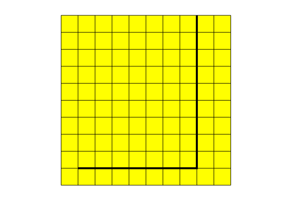
This script illustrates the basic use of the DFM module. We create a simple network of two fractures in a Cartesian 2D grid and add the fracuters to the grid with a hybrid representation. Transmissibilities are then computed with a two-point flux expression, and solve a tracer transport problem. It is assumed that the path is set so that functions in the DFM module will be chosen instead of the core MRST functions. If this is not taken care of, strange error messages will probably result

mrstModule add dfm incomp
gravity reset off;

% Initialize a grid
Nx = [10 10];
G = cartGrid(Nx,[10 10]);
G = computeGeometry(G);

%   Create a fracture at y = 1, and between x = 1 and x = 8
fracFaces = find(all([G.faces.centroids(:,2) == 1 , G.faces.centroids(:,1) >= 1 , ...
    G.faces.centroids(:,1) < 8],2));

%   Create a fracture at x = 8, and between y = 1 and y = 10
fracFaces = [ fracFaces ; find(all([G.faces.centroids(:,1) == 8 , ...
    G.faces.centroids(:,2) >= 1 , G.faces.centroids(:,2) < 10],2))];

%   Mark the face as a fracture face
G.faces.tags=zeros(G.faces.num,1);
G.faces.tags(fracFaces) = 1;

%   Assign aperture
apt = zeros(G.faces.num,1);
aperture = 0.001;
apt(fracFaces) = aperture;

%   Add the hybrid cells
G = addhybrid(G,G.faces.tags > 0,apt);

% Plot the grid and the fracture
figure
plotGrid_DFM(G)
plotFractures(G)
axis equal, axis off

Add physical parameters¶

% Find indices of hybrid cells
hybridInd = find(G.cells.hybrid);

nCells = G.cells.num;

% Define permeability and porosity
rock = makeRock(G, milli*darcy, 0.01);

% The fracture permeability is computed from the parallel plate assumption,
% which states that the permeability is aperture squared divided by 12.
rock.perm(hybridInd,:) = aperture^2/12;
rock.poro(hybridInd) = 0.5;

% Create fluid object. The fluids have equal properties, so this ammounts
% to the injection of a tracer
fluid = initSimpleFluid('mu' , [   1,  1]*centi*poise     , ...
    'rho', [1014, 859]*kilogram/meter^3, ...
    'n'  , [   1,   1]);

% Compute TPFA transmissibilities
T = computeTrans_DFM(G,rock,'hybrid',true);

% Transmissibilites for fracture-fracture connections are computed in a
% separate file
[G,T2] = computeHybridTrans(G,T);

wellRate = 1;
% Injection well in lower left corner, production in upper right
W = addWell([],G,rock,1,'type','rate','val',wellRate,'comp_i',[1 0],'InnerProduct','ip_tpf');
W = addWell(W,G,rock,prod(Nx),'type','rate','val',-wellRate,'comp_i',[0 1],'InnerProduct','ip_tpf');

state = initState(G,W,0,[0 1]);

Solve a single-phase problem, compute time of flight, and plot¶

state = incompTPFA_DFM(state,G,T,fluid,'wells',W,'c2cTrans',T2);

figure
plotCellData_DFM(G,state.pressure)
plotFractures(G,hybridInd,state.pressure)
axis equal, axis off

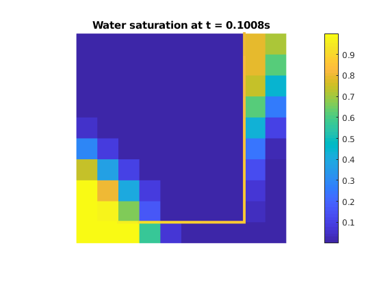
Then solve tracer transport¶

t = 0;

% End of simulation
endTime = sum(0.1 * poreVolume(G,rock) / wellRate);

% Since the two fluids have equal properties, the pressure solution is time
% independent, and the transport equation can be solved for the entire
% simulation time at once. For visualization purposes, we split the
% interval anyhow
numSteps = 5;
dt = endTime / numSteps;

iter = 1;

while t < endTime
    state = explicitTransport_DFM(state,G,t + dt,rock,fluid,'wells',W);

    iter = iter + 1;
    t = t + dt;

    clf
    plotCellData_DFM(G,state.s(:,1));
    plotFractures(G,hybridInd,state.s(:,1));
    axis equal, axis off
    title(['Water saturation at t = ' num2str(t) 's']);
    colorbar

    pause(.1)
end

Copyright notice¶

Unstructured fracture grid created by Matlab functions¶

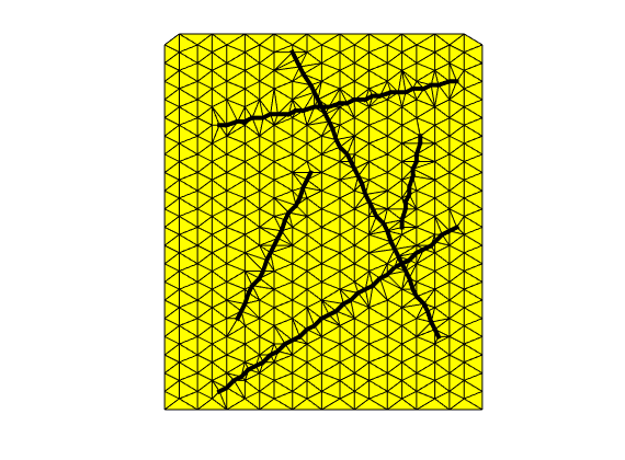
Generated from matlabFractureGrid.m

A somewhat advanced example, where a fracture network is gridded with triangles using a fairly simple approach. The flow equations are then discretized with both two- and multi-point flux expressions, and a two-phase transport problem is solved.

mrstModule add dfm incomp
% Create an initial distribution of points
N     = 20;
N1    = N;
N2    = N;
[X, Y] = meshgrid(0:1:N1, 0:1:N2);
X     = sqrt(3) / 2 * X;
Y(:,2:2:end) = Y(:,2:2:end)+0.5;
p     = [X(:), Y(:)];

% Estimate of the grid size
h = .3;

% Define endpoints of the fractures.
% If a nertex here is also contained in p, one of them should be removed to
% avoid mapping errors in the subsequent Delaunay triangulation
vertices = [ 3 1 ; 16 10 ;...
    3 15.7 ; 16 18 ;...
    15 4 ; 7 19.5  ;...
    4 5  ; 8 13  ;...
    14 15; 13 10];

% Give the constraints wrt numbering of the vertices
constraints = reshape(1 : size(vertices,1),2,[])' ;

% Assign tags to the fractures
constraints = [constraints, (1 : size(constraints,1))'];

% We create the grid by combining the intial points with points distributed
% along the fractures, and gridding the total point cloud with a Delaunay
% algorithm constrained by the fractures. Some tricks are needed to ensure
% the resulting grid has reasonable quality, these are briedly explained
% below. Also note that this strategy does not create high-quality grids,
% for that more advanced methods are needed; see for instance another
% example in the DFM module for a grid created by triangle.

% Bounding box of the domain. Needed for legacy reasons (when the point
% that eventually defines the grid is preconditioned to improve the grid
% quality, points are added to the cloud, and the box is needed to ensure
% the extra points are within the domain).
box = [0 0; N1 N2];

% Cells close the fractures should be significantly larger than the
% apertures for the hybrid DFM approximation to be reasonable. Moreover,
% points that are too close to the fractures will also produce weired
% cells. For these reasons, remove points that are close to the fractures.
% NOTE: The distance from the fractures where we remove points should be
% significantly larger than the tolerance for the fracture location defined
% next.
perimiter = h ;
p = remove_closepoints(vertices,constraints,p,perimiter);

% The quality of the grid is improved if the fractures are alowed to
% deviate somewhat from straight lines. This is of course an approximation,
% but it is in agreement with a concept of uncertainty in the fracture
% description. This parameter is more important for more advanced
% gridding algorithms than the present one. Still, reducing this value will
% make the fractures closer to straight lines
args = struct('precision',0.01);

% Add vertices in the intersection between fractures
[vertices, constraints] = removeFractureIntersections(vertices,constraints,box,args);

numOrdPt = size(p,1);

% Concatenate the prescribed points and the fracture endpoints
p  = [p ; vertices];

% Let constraints refer to the new point distribution
constraints(:,1:2) = constraints(:,1:2) + numOrdPt;

% Add points along the fractures to get reasonable grids there as well
[p, constraints, map] = partition_edges(p,constraints,0.5,box,args);

% Bookkeeping
tags = constraints(:,3);
constraints =  constraints(:,1:2);

% Now the points are defined. Create a constrained Delauny triangulation
% on the point cloud, and create the grid
delTri     = DelaunayTri(p, constraints);
G     = triangleGrid(delTri.X, delTri.Triangulation);
G = computeGeometry(G);

Introduce hybrid representation of fractures¶

G.faces.tags = zeros(G.faces.num,1);

% Recover faceNodes, and sort the nodes columnwise (for the use of ismember
% later)
faceNodes = sort(reshape(G.faces.nodes,2,[])',2);

% Use constraints from the Delaunay triangulation, in case these have been
% changed (it shouldn't happen, and will give a warning)
% Rowwise sort to prepare for using ismember
constraints = sort(delTri.Constraints,2);

% Loop over all constraints (the segments of fractures) and find the faces
% that spans the constraint.
for iter = 1 : size(constraints)
    % ismember works here since both inputs have been sorted
    fracFace = find(ismember(faceNodes,constraints(iter,:),'rows'));

    % Assign a tag to the newly found fracture face
    G.faces.tags(fracFace) = tags(iter);
end

% Apertures of all faces. Zero aperture for non-fractures
aperture = zeros(G.faces.num,1);

% Set different apertures for each
for iter = unique(tags)'
    hit = G.faces.tags == iter;
    aperture(hit) = 10^-3 * rand(1); % This choice is random in more than one way..
end

% Add hybrid cells along the fractures
G = addhybrid(G,G.faces.tags > 0,aperture);

% Plot the grid and the fracture. Note that the fracuters are not straight
% lines.
figure
plotGrid_DFM(G)
plotFractures(G)
axis equal, axis off

Set parameters¶

% Find indices of hybrid cells
hybridInd = find(G.cells.hybrid);
nCells = G.cells.num;

% Define permeability and porosity
rock = makeRock(G, [1, 1]*milli*darcy, 0.01);

% Much higher values are used in the fracture
rock.perm(hybridInd,:) = aperture(G.cells.tags(hybridInd)).^2/12 * [1 1];
rock.poro(hybridInd) = 0.5;

% Create fluid object. Non-linear rel perms, resident fluid has the higher
% viscosity
fluid = initSimpleFluid('mu' , [   2,  2]*centi*poise     , ...
    'rho', [1014, 859]*kilogram/meter^3, ...
    'n'  , [   1,   10]);

Define wells¶

% Well rate
wellRate = 1;

% Place both injection and production wells close to the fracture network
injInd = delTri.pointLocation(3, 1);
prodInd = delTri.pointLocation(16, 17);

W = addWell([],G,rock,injInd,'type','rate','val',wellRate,'comp_i',[1 0],'InnerProduct','ip_simple');
W = addWell(W,G,rock,prodInd,'type','rate','val',-wellRate,'comp_i',[0 1],'InnerProduct','ip_simple');

state = initState(G,W,0,[0 1]);

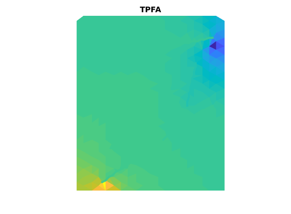
Compute transmissibilities with both MPFA and TPFA¶

% Note that there is a difference in how connections between hybrid cells
% are handled between TPFA and MPFA: Both methods discretize the
% connections in files that are separate from compute(MP)Trans, but TPFA
% gives a separate list of transmissibilities for cell-to-cell connections,
% whereas MPFA modifies the standard transmissibility matrix.

% Transmissibilities with TPFA
T_TPFA = computeTrans_DFM(G,rock,'hybrid',true);
[G,T_TPFA_2] = computeHybridTrans(G,T_TPFA);
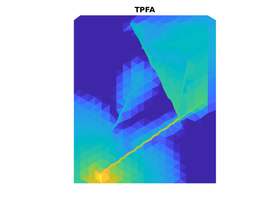
state_TPFA = incompTPFA_DFM(state,G,T_TPFA,fluid,'wells',W,'c2cTrans',T_TPFA_2);

figure
plotCellData_DFM(G,state_TPFA.pressure)
plotFractures(G,hybridInd,state_TPFA.pressure)
title('TPFA')
axis off, axis equal
%
% % Transmissibilities with MPFA
% T_MPFA = computeMultiPointTrans_DFM(G,rock,'hybrid',true);
% [G,T_MPFA] = computeHybridMPTrans(G,T_MPFA);
% state_MPFA = incompMPFA_DFM(state,G,T_MPFA,fluid,'wells',W,'cellConnections',true);
%
% figure
% plotCellData_DFM(G,state_MPFA.pressure)
% plotFractures(G,hybridInd,state_MPFA.pressure)
% title('TPFA')
% axis off, axis equal

Solve two-phase problem.¶

% Comments are sparse here, for explanations see examples in the core files
% of MRST.
% The plotting is designed to highlight differences between two- and
% multi-point fluxes

t = 0;

% Simulation endtime
T = 0.02 * sum(poreVolume(G,rock)) / wellRate;

numTimeSteps = 100;
dt = T / numTimeSteps;

numSatPlots = 3;
dtSatPlot = T / numSatPlots;

nextSatPlot = dtSatPlot;

% Store concentration in the outlet
wellConcentration = zeros(numTimeSteps + 1,2);

% Transport loop.
while t < T
    % Transport solve with both methods. We use implicit transport to avoid
    % severe time step restrictions due to high flow rates and small cells
    state_TPFA =  implicitTransport_DFM(state_TPFA,G,t + dt,rock,fluid,'wells',W);
%     state_MPFA =  implicitTransport_DFM(state_MPFA,G,t + dt,rock,fluid,'wells',W);

    wellConcentration(iter + 1,1) = state_TPFA.s(prodInd,1);
%     wellConcentration(iter + 1,2) = state_MPFA.s(prodInd,1);

    % Update pressure solution
    state_TPFA = incompTPFA_DFM(state_TPFA,G,T_TPFA,fluid,'wells',W,'c2cTrans',T_TPFA_2);
%     state_MPFA = incompMPFA_DFM(state_MPFA,G,T_MPFA,fluid,'wells',W,'cellConnections',true);

    iter = iter + 1;
    t = t + dt;

    % Plotting
%     if t >= nextSatPlot
        figure(1); clf
%         subplot(2,1,1)
        plotCellData_DFM(G,state_TPFA.s(:,1));
        plotFractures(G,hybridInd,state_TPFA.s(:,1));
        title('TPFA')
        axis off, axis equal
        drawnow
%
%         subplot(2,1,2)
%         plotCellData_DFM(G,state_MPFA.s(:,1));
%         plotFractures(G,hybridInd,state_MPFA.s(:,1));
%         title('MPFA')
%         axis off, axis equal
%
%         nextSatPlot = nextSatPlot + dtSatPlot;
%     end

end

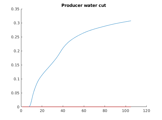
% Finally plot water cuts in the producer
figure, hold on
plot(wellConcentration(:,1))
plot(wellConcentration(:,2),'r')
title('Producer water cut')

Copyright notice¶

<html>
% <p><font size="-1

dfm: Discrete fracture matrix implementation¶

Examples¶

Basic Cartesian fracture grid¶

Add physical parameters¶

Solve a single-phase problem, compute time of flight, and plot¶

Then solve tracer transport¶

Copyright notice¶

Unstructured fracture grid created by Matlab functions¶

Introduce hybrid representation of fractures¶

Set parameters¶

Define wells¶

Compute transmissibilities with both MPFA and TPFA¶

Solve two-phase problem.¶

Copyright notice¶

`dfm`: Discrete fracture matrix implementation¶