hfm: Hierarchical and embedded fractures
The hierarchical fracture module (HFM) utilises the hierarchical fracture modelling framework to simulate multiphase flow in naturally fractured reservoirs with multiple length scales. Also known as the embedded discrete fracture model, this method models fractures explicitly, as major fluid pathways, and benefits from independent definitions of the fracture and matrix grid. As a result, intricate fracture networks can be modelled easily, without the need for a complex underlying matrix grid that is conformal with each fracture. The module also extends the newly developed multiscale restriction smoothed basis (MsRSB) method to compute the flux field developed in a fractured reservoir. The multiscale approach of dealing with fractures is inspired by similar strategies developed for the multiscale finite volume (MSFV) method.
-
checkDistmesh()¶ Checks if distmesh_2d file is installed in the MATLAB path
Synopsis:
hasLSI = checkLineSegmentIntersect();
checkLineSegmentIntersect();
Description:
This function checks if the file ‘distmesh_2d.m’ (http://people.sc.fsu.edu/~jburkardt/m_src/distmesh/distmesh.html) is installed in the current MATLAB path and advises the user to install it if it is not found.
If called with a return argument, it will produce a boolean indicating the status of the distmesh_2d.m file. The application checking for distmesh_2d.m can then fall back to other implementations of graph algorithms as they please. If called without any return arguments, it will throw an error if distmesh_2d.m was not found, along with a link and install instructions for the user to rectify the missing installation.
Returns: foundLSI (OPTIONAL) – If distmesh_2d.m was found. Note that the nature of the utility changes if called with return argument.
-
checkIfCoplanar(fracplanes)¶ Asserts that a given set of points (in 3D) are coplanar.
-
checkLineSegmentIntersect()¶ Checks if lineSegmentIntersect file is installed in the MATLAB path
Synopsis:
hasLSI = checkLineSegmentIntersect();
checkLineSegmentIntersect();
Description:
This function checks if the file ‘lineSegmentIntersect.m’ (http://www.mathworks.com/matlabcentral/fileexchange/27205) is installed in the current MATLAB path and advises the user to install it if it is not found.
If called with a return argument, it will produce a boolean indicating the status of the lineSegmentIntersect.m file. The application checking for lineSegmentIntersect.m can then fall back to other implementations of graph algorithms as they please. If called without any return arguments, it will throw an error if lineSegmentIntersect.m was not found, along with a link and install instructions for the user to rectify the missing installation.
Returns: foundLSI (OPTIONAL) – If lineSegmentIntersect.m was found. Note that the nature of the utility changes if called with return argument.
-
checkMATLABversionHFM()¶ Checks if the matlab version is greater than 2015a for compatibility with ‘ismembertol’ and ‘uniquetol’ functions and prints a warning if the matlab version is lower.
Synopsis:
v = checkMATLABversionHFM();
checkMATLABversionHFM();
Returns: v (OPTIONAL) – Matlab version as a character array (ex: 2015a)
-
computeEffectiveTrans(G)¶ Computes the effective transmissibility between the fracture and matrix by harmonically averaging weighted permeablities and multiplying by CI.
-
establishSign(G, fracplanes, varargin)¶ Assigns a value of 0 (if the node/edge lies on the plane), 1 (if the node/edge lies on the positive side of the plane) or -1 (if the node/edge lies on the negative side of the plane) to every corner point and edge of the input polygon with respect to the normal vector of the polygon and the normal vector of its bounding planes.
-
extend_frac2D(G, frac_endp, edges, out, cnum, cnodes, faces)¶ extend_frac is used to extend a 2D fracture line when it only partially penetrates matrix cells at its end points. Following this, the ratio of true fracture length to its extended length inside the concerned matrix cell is returned. CI is computed for the extended fracture inside the corresponding matrix cell and scaled by this ratio. See Lee et al, Water Resources Research, 2001.
-
findRectangularFractures(fractures)¶ Indicates the rectangular fractures using a structure containing, for each fracture, the set of points defining the fracture polygon in 3D.
-
generatePointsOnPlane(points, varargin)¶ Generates points on a 3D convex polygon defined by a coplanar set of points
-
getAvgFracDist2D(G, fracp, cell_num, cnodes)¶ getAvgFracDist computes the average normal distance of each point inside a matrix cell from every fracture line that intersects with this cell. This is the same as <d> used for computing conductivity index (CI, see CIcalculator2D) as described in SPE-103901-PA, Lyong Li and Seong H. Lee, 2008.
-
getPlaneNormals(fracplanes, varargin)¶ Computes the normal vector for a set of coplanar points in 3D. Additionally, it returns the normal vector of the bounding planes perpendicular to the edges of the polygon defined by the set of input points.
-
globalTriangulation(G)¶ This function creates a global triangulation such that each cell in a grid is made up of one or more full tetrahedrons. The global triangulation can then be used to locate the cells that enclose a given set of points.
-
inPolygon3D(q, p, varargin)¶ Indicates if a set of query points ‘q’ in 3D lie inside or on a polygon defined by coplanar points ‘p’.
-
iscoplanar(pxyz, varargin)¶ Checks if a set of points lie on the plane defined by points ‘pxyz’ and returns an indicator value for each point along with its normal distance from the plane.
-
makeRockFrac(G, K_frac, varargin)¶ makeRockFrac can be used to set homogeneous rock properties to the fracture grid stored in G.FracGrid given a scalar value for fracture permeability and porosity.
Synopsis:
G = makeRockFrac(G, K_frac)
G = makeRockFrac(G, K_frac, 'pn1', 'pv1')
G = makeRockFrac(G, K_frac, 'pn1', 'pv1', 'pn2', pn2)
Parameters: - G – Grid data structure containing fracture grids (for each fracture line or plane) in G.FracGrid
- K_frac – Scalar Darcy permeability for homogeneous fractures.
Keyword Arguments: - permtype – ‘homogeneous’ or ‘heterogeneous’. If ‘heterogeneous’ is passed as the permtype, this function assigns a random permeability distribution to each fracture grid cell. To manually assign a specific permeability distribution, the user must access G.FracGrid.Frac#.rock.perm as shown in the code written below. In that case, one does not need to call makeRockFrac.
- porosity – Scalar value for rock porosity (0<porosity<1)
Returns: G – Grid data structure with structure rock added to each fracture grid (Frac#) in G.FracGrid.
Note
This function uses randi() to generate a random permeability field when ‘heterogeneous’ is specified as ‘permtype’.
See also
FracTensorGrid2D
-
pdist_euclid(x)¶ Pairwise euclidian distance between pairs of objects.
-
polyArea3D(p)¶ Computes the surface area of a polygon defined by the set of points ‘p’ in 3D
-
rotatePlane(points, normal, varargin)¶ Rotates a set of points (assumed to be coplanar) in order to align with a plane defined by the input normal vector. Rotation is along the axis defined by the intersection of the two planes. If the plane defined by the input set of points is parallel to the input normal vector, then this function returns the points without making a transformation.
-
roundsd(x, n, method)¶ ROUNDSD Round with fixed significant digits ROUNDSD(X,N) rounds the elements of X towards the nearest number with N significant digits.
- ROUNDSD(X,N,METHOD) uses following methods for rounding:
- ‘round’ - nearest (default) ‘floor’ - towards minus infinity ‘ceil’ - towards infinity ‘fix’ - towards zero
Example:
roundsd(0.012345,3) returns 0.0123
roundsd(12345,2) returns 12000
roundsd(12.345,4,'ceil') returns 12.35
See also Matlab’s functions ROUND, ROUND10, FLOOR, CEIL, FIX, and ROUNDN (Mapping Toolbox).
- Author: Franois Beauducel <beauducel@ipgp.fr>
- Institut de Physique du Globe de Paris
Acknowledgments: Edward Zechmann, Daniel Armyr, Yuri Kotliarov
Created: 2009-01-16 Updated: 2015-04-03
-
translateLine(points, a)¶ translateLine(points,a) translates the line given by an n-by-2 vector of coincident ‘points’ by a normal distance ‘a’ in 2D space to create a rectangle given by the 2*n-by-2 vector ‘p’.
-
tri_area(P1, P2, P3)¶ tri_area(P1, P2, P3) calculates the triangle area given the coordinates of its vertices in P1, P2 and P3 using Heron’s formula.
Heron’s Formula: s = semiperimeter A = sqrt(s * (s-a) * (s-b) * (s-c)) Where a,b,c are lengths of the triangle edges
-
addCoarseCenterPointsFrac(CGf, varargin)¶ addCoarseCenterPointsFrac adds coarse nodes to the fracture coarse grid CGf. This function can be modified to improve coarse node selection inside fractures.
Synopsis:
CGf = addCoarseCenterPointsFrac(CGf)
CGf = addCoarseCenterPointsFrac(CGf, 'pn1', 'pv1', ...)
Parameters: CGf – Fracture coarse grid (supplied by ‘generateCoarseGrid’) with geometry information (computed through ‘coarsenGeometry’).
Keyword Arguments: option – option specifies the type of coarse grid points to use for computing the coarse node location. Possible self-explanatory values are:
- ‘useCoarseFaceCentroids’
- ‘useCoarseCellCentroids’
- ‘useFineCellCentroids’
- ‘useCoarseCellEndPoints’ - 2D grids only
passed as character arrays.
meantype – type of mean, of the points specified by option, to use for computing the coarse node location. Valid input values include ‘geometric’ and ‘arithmetic’ passed as character arrays. This option is not useful if ‘useCoarseCellEndPoints’ is passed as the option
Returns: CGf – Fracture coarse grid with CGf.cells.centers added as a new field.
See also
storeFractureInteractionRegion
-
getRsbGridsHFM(G, nw, varargin)¶ Computes coarse grid and interaction region for a grid with fractures
- SYNOPSIS:
- [CG, CGf] = getRsbGridsHFM(G, nw) [CG, CGf] = getRsbGridsHFM(G, nw, ‘pn1’, pv1, …)
- DESCRIPTION:
- This function coarsens the matrix and fracture grids separately and computes support regions for the fracture and matrix basis functions. All of this is then combined into one coarse grid to be used for the multiscale solver. There are no restrictions on grid definition. Fracture partitioning algorithms are graph based.
REQUIRED PARAMETERS:
G - Grid structure with fractures as defined by assembleGlobalGrid.
- nw - Structure containing indices of fractures that make up every
- independent fracture network. same as fracture.networks for 2D examples (see getIndepNetwork)
OPTIONAL PARAMETERS:
- pm - Partition vector mapping matrix fine cells to coarse blocks.
- Size = nm-by-1 where nm is the total number of fine cells in the matrix.
- coarseDims - Number of coarse blocks in each physical direction.
- Assumed to be a LENGTH 2 or 3 vector of integers. To be used only when the matrix grid is structured.
- sampleDims - Hypothetical cartesian dimensions (specifying number of
- fine-cells in each coordinate direction) representing a unstructured grid. Used to construct a structured coarse grid, in the same physical space, which is then utilized as a sample for mapping the unstructured fine grid to the structured coarse grid. See sampleFromBox.
- use_metis - Logical value (true or false) to indicate the use of
- metis to partition matrix.
- dof_matrix - Degrees of freedom in matrix at coarse scale. Required if
- use_metis = true.
- MatrixTrans - Transmissibility vector for all fine-grid faces in the
- matrix
- partition_frac - Logical value to indicate if fractures must be
- coarsened. Otherwise fractures will be a part of the matrix coarse grid and support regions and there will be no coarse nodes inside a fracture. Useful to observe the impact of coarsening fractures.
- coarseDimsF - Number of coarse blocks for a fracture plate in each
- physical direction. Aplicable only to rectangular fracture plates in 3D system.
- sampleDimsF - Similar to its counterpart in the matrix. Aplicable only
- to rectangular fracture plates in 3D system.
- use_metisF - Logical value (true or false) to indicate the use of
- metis to partition fractures.
- dof_frac - Degrees of freedom in each fracture network at coarse
- scale. Required when use_metisF = true. Must either be a single value < minimum number of fine cells in all independant fracture networks or a vector containing a value for each intependent fracture network.
- sysMatrix - Fine scale system (transmissibility) matrix A (see
- incompTPFA). Not necessary, but if available, allows the use of an existing variable to construct an Adjacency (or connectivity) matrix.
- fracSupportRadius - levels of connectivity used to define the support
- region for a fracture coarse block. In other words, the topological radius of the fracture support region. See storeFractureInteractionRegion.
- fullyCoupled - Coupled fracture and matrix basis functions. Allows
- matrix support to extend into fractures. Increases accuracy but reduces speed.
- excludeBoundary - Excludes fine cells on the boundary from support
- regions of internal coarse blocks. Improves accuracy, especially when boundary conditions are specified.
———–EXPERIMENTAL———–%%%%%%%%%%%%%%%%%%%%%%
- removeCenters - Logical value to essentially enforce a basis
- function value of 1 at each coarse node. May improve convergence rate in an iterative multiscale strategy.
- coarseNodeOption - Possible methods for optimizing coarse node location
- inside fractures.
- paddedPartition - If true, uses partitionUniformPadded to partition
- matrix coarse grid. Requires ‘coarseDims’.
- paddedPartitionF - If true, uses partitionUniformPadded to partition
- fracture coarse grid. Requires ‘coarseDimsF’.
Wells - Well structure. See addWell.
- nearWellRefinement - Refines the coarse grid near wells by recursively
- splitting the coarse block containing a well a specified number of times.
- nearWellRefinementMultipler - Integer denoting the number of times the
- coarse block containing a well must be recursively split into 2.
- RETURNS:
- CG - Coarse grid for grid G with basis supports and coarse node
- indices. See storeInteractionRegion, generateCoarseGrid.
- CGf - Fracture coarse grid with similar information as CG but only for
- the internal fracture grid Gf as returned by assembleFracGrid.
- SEE ALSO:
- partitionMatrix, partitionFracture, generateCoarseGrid, storeInteractionRegion, storeInteractionRegionFrac, partitionMETIS, callMetisMatrix.
-
getRsbGridsMatrix(G, pm, varargin)¶ Generates the matrix coarse grid and computes support regions for the matrix coarse blocks. See generateCoarseGrid and storeInteractionRegion.
-
partitionFracture(G, pm, nw, varargin)¶ Generates partition vector for the fracture grid. See getRsbGridsHFM for description of input parameters.
-
partitionMatrix(G, varargin)¶ Generates partition vector for the matrix grid. See getRsbGridsHFM for description of input parameters.
-
storeFractureInteractionRegion(CG, CGf, CGm, varargin)¶ - storeFractureInteractionRegion defines and stores connectivity or grid
topology based internal and external (matrix) support regions for a given matrix and fracture coarse grid.
- SYNOPSIS:
- [CG,CGf] = storeFractureInteractionRegion(CG, CGf, CGm) [CG,CGf] = storeFractureInteractionRegion(CG, CGf, CGm, ‘pn1’, pv1, …)
- DESCRIPTION:
- This function computes the support for fracture basis functions including interaction in the matrix as well as internal to each fracture network.
REQUIRED PARAMETERS:
CG - Coarsened global grid ‘G’ containing fracture and matrix cells.
CGf - Coarsened fracture grid ‘Gf’ defined by assembleFracGrid.
CGm - Matrix coarse grid.
OPTIONAL PARAMETERS:
- levels - levels of connectivity used to define the support region
- for a fracture coarse block. In other words, the topological radius of the fracture support region.
- fullyCoupled - Coupled fracture and matrix basis functions. Allows
- matrix support to extend into fractures. Increases accuracy but reduces speed.
- excludeBoundary - Excludes fine cells on the boundary from support
- regions of internal coarse blocks. Improves accuracy, especially when boundary conditions are specified.
———–EXPERIMENTAL———–%%%%%%%%%%%%%%%%%%%%%%
- removeCenters - Logical value to essentially enforce a basis
- function value of 1 at each coarse node. May improve convergence rate in an iterative multiscale strategy.
- coarseNodeOption - Possible methods for optimizing coarse node location
- inside fractures.
- RETURNS:
- CG - Coarse grid for combined fracture and matrix grid ‘G’ with basis
- supports and coarse node indices in added fields ‘G.cells.interaction’ and ‘G.cells.centers respectively’.
- CGf - Fracture coarse grid with similar added information as CG but
- only for the internal fracture grid Gf as returned by assembleFracGrid.
- SEE ALSO:
- storeInteractionRegion, getRsbGridsHFM, storeFractureInternalInteractionRegion, addCoarseCenterPointsFrac
-
storeFractureInternalInteractionRegion(CGf, G, A, varargin)¶ storeFractureInternalInteractionRegion can be used to compute the support region that lies inside a fracture for every fracture coarse block.
Synopsis:
CGf = storeFractureInternalInteractionRegion(CGf, G, A)
CGf = storeFractureInternalInteractionRegion(CGf, G, A, 'pn1', 'pv1', ...)
Parameters: CGf – Fracture coarse grid (supplied by ‘generateCoarseGrid’) with geometry information (computed through ‘coarsenGeometry’).
Keyword Arguments: - simpleInteractionRegion – connects neighboring coarse nodes, in a 2D domain where fractures are represented as 1D grids to compute the interaction region.
- callStoreInteractionRegion – calls the function storeInteractionRegion to compute fracture internal interaction regions. Applicable for 3D domains.
Returns: CGf – Fracture coarse grid containing internal support regions in the list CGf.cells.interaction.
See also
storeInteractionRegionFrac
-
CIcalculator2D(G, fracture, varargin)¶ CIcalculator2D computes the conductivity index (CI) of each 2D cell for every fracture line embedded in it.
Synopsis:
G = CIcalculator2D(G,fracture)
G = CIcalculator2D(G,fracture, waitbar)
Description:
CI or conductivity index is similar to the well productivity index as in the Peaceman well model. In hierarchical/embedded fracture modelling, the flux exchange between fracture and matrix is defined by a model similar to the peaceman well model. See Lee et al, Water Resources Research, 2001 or SPE-65095-PA, Lee et al, 2000.
Parameters: - G – Matrix grid structure as returned by processFracture2D.
- fracture – Processed fracture structure. See processFracture2D.
- waitbar – Display a waitbar if this boolean variable is true
Returns: G – Matrix grid structure with added cell lists ‘G.cells.fracture.CI’ and ‘G.cells.fracture.fA’ containing fracture-matrix conductivity index and fracture length inside each matrix cell respectively
See also
processFracture2D, getIndepNetwork, markcells2D
-
defineNNCandTrans(G, F, fracture)¶ defineNNCandTrans identifies fracture-matrix and fracture-fracture connections and computes once transmissibility for each connections.
Synopsis:
[G,T] = defineNNCandTrans(G,F,fracture)
Description:
defineNNCandTrans first recognizes all fracture-matrix connections and stores them as non-neighboring connections (NNC’s). Then, the global grid ‘G’ containing both fracture and matrix grid cells is assembled. Following that, fracture-fracture connections (at intersections) are defined as NNC’s and added to the global grid. The script also computes transmissibilities for these NNC’s using rock properties defined in G. This function calls frac_matrix_nnc, frac_frac_nnc, assembleGlobalGrid and computeTrans internally.
Parameters: - G – Grid data structure containing G.FracGrid (see FracTensorGrid2D) with corresponding rock properties and G.cells.fracture (see markcells2D and CIcalculator2D).
- fracture (F,) – Output from gridFracture2D.
Returns: - G – Global grid structure (individual matrix and fracture grids assembled into 1 grid) with NNC’s and relevant information defined in G.nnc.
- T – Face transmissibilities.
See also
gridFracture2D, assembleGlobalGrid, frac_matrix_nc, frac_frac_nnc
-
fracMatrixConnections(G, Gfrac, CItot, possible_cells, area, varargin)¶ fracMatrixConnections assigns a “non-neighboring connection (NNC)” status to each fracture-matrix connection and also assigns a transmissibility to each NNC given the total conductivity index of the fracture. See Lee et al, Water Resources Research, 2001 or SPE-65095-PA, Lee et al, 2000.
-
frac_frac_nnc(G, F, fracture)¶ frac_frac_nnc assigns NNC connections to fracture-fracture intersections and also assigns a transmissibility to each connection using the star-delta transformation. See see SPE-88812-PA, Karimi-Fard et al, 2004.
Synopsis:
G = frac_frac_nnc(G,F,fracture)
Parameters: - G – Grid data structure containing G.FracGrid (see FracTensorGrid2D) and corresponding rock properties for the fracture.
- fracture (F,) – Output from gridFracture2D.
Returns: G – Grid structure with fracture-fracture intersections and their transmissibilities added in the cell lists ‘G.nnc.cells’ and ‘G.nnc.T’ respectively. To aid in detecting specific NNC types, these connections are added as ‘star-delta’ type in the list ‘G.nnc.type’
See also
assembleFracNodes2D, gridFracture2D, frac_matrix_nnc
-
frac_frac_nnc_extruded(G, Gl, F, fracture, flayers)¶ frac_frac_nnc_extruded assigns NNC connections to fracture-fracture intersections (similar to its 2D counterpart frac_frac_nnc) and also assigns a transmissibility to each connection using the star-delta transformation. See see SPE-88812-PA, Karimi-Fard et al, 2004. The NNC’s are first identified in 2D and then extruded to 3D.
-
frac_matrix_nnc(G, F, fracture)¶ frac_matrix_nnc assigns a “non-neighboring connection (NNC)” indicators to each fracture-matrix connection and also assigns a transmissibility to each NNC. See Lee et al, Water Resources Research, 2001 or SPE-65095-PA, Lee et al, 2000.
Synopsis:
G = frac_matrix_nnc(G,F,fracture)
Parameters: - G – Grid data structure containing G.FracGrid (see FracTensorGrid2D) and G.cells.fracture (see markcells2D and CIcalculator2D)
- fracture (F,) – Output from gridFracture2D.
Returns: G – Grid structure with fracture-matrix connections at fine scale and their corresponding CI added in ‘G.nnc’ as lists ‘G.nnc.cells’ and ‘G.nnc.CI’ respectively. To aid in detecting specific NNC types, these connections are added as ‘frac-matrix’ type in the list G.nnc.type
See also
getIndepNetwork, markcells2D, CIcalculator2D, gridFracture2D, frac_frac_nnc
-
getIndepNetwork(fl)¶ getIndepNetwork(fl) extracts independant fracture networks from a set of ‘n’ fracture lines given by an n-by-4 matrix with each row containing the end points of a fracture line. This function is used when the matrix is two-dimensional.
Synopsis:
frac = getIndepNetwork(fl)
Parameters: fl – fracture lines represented by it’s end points as [x1 y1 x2 y2]. fl will have 1 row per fracture line.
Returns: frac – Structure containing information about individual fractures with the following sub-structures: (a) lines - Structure with the fields “network”
(network to each fracture belongs), “endp” (endpoints of each fracture line as supplied by ‘fl’) and “cells” (matrix cells containing the fracture) . Size = 1-by-rows(fl).
- network - stores indices for fracture lines contained in
- each network.
See also
markcells2D
-
makeLayers(G, nl, flayers)¶ This function extrudes the matrix grid and independent fracture grid given the number of layers.
Synopsis:
Gl = makeLayers(G,nl,flayers)
Parameters: - G – Matrix grid structure post fracture processing and gridding.
- nl – Number of extruded layers.
- flayers – Indices of extruded layers in which fractures are present.
Returns: Gl – Extruded matrix grid structure with extruded fracture grids stored in Gl.FracGrid.
See also
makeLayeredGrid
-
makeNNCextruded(G, Gl, F, fracture, flayers)¶ makeNNCextruded identifies fracture-matrix and fracture-fracture connections and computes a single transmissibility for each connection.
Synopsis:
[Gl,T] = makeNNCextruded(G,Gl,F,fracture,flayers)
Description:
defineNNCandTrans first recognizes all fracture-matrix connections in 2D and stores them as non-neighboring connections (NNC’s) following which these connections are added to the layerd grid. Then, the global grid ‘G’ containing both fracture and matrix grid cells (in 3D) is assembled. Next, fracture-fracture connections (at intersections) are defined as NNC’s and added to the global grid. The script also computes transmissibilities for these NNC’s using rock properties defined in G. This function calls frac_matrix_nnc, frac_frac_nnc, assembleGlobalGrid and computeTrans internally.
Parameters: - G – Grid data structure containing G.FracGrid (see FracTensorGrid2D) with corresponding rock properties and G.cells.fracture (see markcells2D and CIcalculator2D)
- Gl – Extruded matrix and fracture grids. See makeLayers
- fracture (F,) – Output from gridFracture2D.
- flayers – Indices of extruded layers in which fractures are present.
Returns: - Gl – Global extruded grid structure with matrix and fracture assemblies combined into a single grid. NNC’s and other relevant information is defined in G.nnc.
- T – Face transmissibilities.
See also
assembleGlobalGrid, frac_matrix_nc, frac_frac_nnc_extruded, makeLayers
-
markcells(G, fracplanes, varargin)¶ markcells returns the indices of matrix cells that are connected with each fracture.
-
markcells2D(G, frac)¶ markcells2D assigns a indicator to cells containing embedded fractures or discrete fractures at any of its faces. Indices of fracture lines and networks are also stored for the corresponding cells. Each fracture is assumed to be a line by this function. See processFracture2D for details on input and output.
-
preProcessingFractures(G, fracplanes, varargin)¶ preProcessingFractures identifies fracture-matrix connections, imposes a fracture grid and computes the fracture-matrix conductivity index.
Synopsis:
[G,fracplanes] = preProcessingFractures(G, fracplanes)
[G,fracplanes] = preProcessingFractures(G, fracplanes, 'pn1', pv1)
Parameters: - G – Grid data structure containing geometrical information.
- fracplanes – 1-by-n structure where n is the number of fractures. Each column contains a set of coplanar points that define the fracture polygon and a value for the fracture aperture.
Keyword Arguments: fractureGridType – Type of fracture mesh desired. Possible options: (a) 1 - Cartesian mesh: Possible only when the fracture plane is rectangular.
(b) 2 - Triangle mesh: Uses the external library ‘distmesh’ to create the nodes and connectivity list required to create a triangular grid.
(c) 3 - PEBI mesh: Voronoi grid. External library ‘distmesh’ required to create underlying triangulation.
fractureCellSize – Dimensionless element size (>0 and <1) for the fracture grid.
GlobTri – See globalTriangulation.
pointDensity – A measure to control the number density of points generated on a fracture plane for processing purposes.
inPolygonTolerance – Tolerance for checking if a set of points lie inside a polygon.
uniqueTolerance – Tolerance for the matlab function unique.
Returns: - G – Grid data structure with added fields G.nnc and G.FracGrid. G.FracGrid contains the grid information for each fracture. G.nnc contains relevant information about fracture matrix connections, which are defined as NNC’s to compute transmissibilities.
- fracplanes – Structure with added fields normal and boundNormals for each fracture polygon.
See also
markcells, getPlaneNormals, gridPlanarFracture, fracMatrixConnections
-
processFracture2D(G, fl, varargin)¶ processFracture2D extracts independant fracture networks and stores matrix cells containing fractures given a matrix grid and a set of fracture lines in two dimensions.
Synopsis:
[G,fracture] = processFracture2D(G, fl)
[G,fracture] = processFracture2D(G, fl, 'pn1', pv1)
Parameters: - G – Grid data structure.
- fl – fracture lines represented by it’s end points as [x1 y1 x2 y2]. fl will have 1 row per fracture line. Size = nf-by-1.
Keyword Arguments: verbose – Enable output. Default value dependent upon global verbose settings of function ‘mrstVerbose’.
Returns: G – Grid data structure with an added cell list G.cells.fracture containing indicator values for cells containing fractures as well as the indices of those fractures.
fracture –
- Structure containing information about individual fractures
with the following sub-structures:
- lines - Structure with the fields “network”
- (network to each fracture belongs), “endp” (endpoints of each fracture line as supplied by ‘fl’) and “cells” (matrix cells containing the fracture) . Size = 1-by-rows(fl).
- network - stores indices for fracture lines contained in
- each network.
Note
This function calls getIndepNetwork and markcells2D internally.
See also
getIndepNetwork, markcells2D
-
FracTensorGrid2D(G, F, a, varargin)¶ FracTensorGrid2D uses information about each fracture line supplied by ‘F’ obtained through assembleFracNodes2D and creates a tensorGrid for each fracture line using the fracture aperture ‘a’.
Synopsis:
G = FracTensorGrid2D(G,F,a)
G = FracTensorGrid2D(G,F,a,'plot')
Parameters: - G – Matrix grid data structure.
- F – Structure containing information abo’Frac’ut partitioned fracture lines as returned by assembleFracNodes2D.
- a – Fracture aperture, Must either have a single value for all fracture lines or an individual value for each fracture line. Varying fracture apartures for one line are not supported.
OPTIONAL PARAMETER:
‘plot’ - Plot all fracture grid structures returned under G.FracGrid.Returns: G – Grid structure with sub-structure G.FracGrid. G.FracGrid in-turn contains a grid structure for each fracture line with nomenclature such as Frac1, Frac2, and so on. G.FracGrid.Frac1, for example, will have the same basic grid structure as G. See also
assembleFracNodes2D, tensorGrid
-
assembleFracGrid(G)¶ assembleFracGrid assembles a grid (Gf) containing only fractures using the global grid (G) containing both fracture and matrix information.
Synopsis:
Gf = assembleFracGrid(G)
Parameters: G – Grid structure with fractures (see assembleGlobalGrid) Returns: Gf – Grid structure containing all fracture lines as 1 grid. Note
This function assumes that each fracture grid is represented as a cartesian grid. Underlying matrix grid structure as in ‘G’ can be cartesian or unstructured. Fracture intersections exist as NNC’s (Gf.nnc.cells) in the returned grid Gf. Transmissibility at these intersections can also be found in Gf.nnc. Fracture-matrix connections do not exist in the output grid.
See also
assembleGlobalGrid
-
assembleFracNodes2D(G, fracture, varargin)¶ assembleFracNodes2D partitions fracture lines to generate nodes for gridding
Synopsis:
[F,fracture] = assembleFracNodes2D(G, fracture);
[F,fracture] = assembleFracNodes2D(G, fracture, 'pn1', pv1, ...);
Description:
This function supports 3 possible options to divide a fracture for gridding. The resulting output can be thought of as a 1D grid for each fracture line. From preliminary experiments, option/type 1 has proved to be the cheapest way to ensure relatively uniform gridding with similar resolution throughout all fractures. For each assemblyType fracture intersections will be a node on each of the intersecting line. This is because transmissibility at these intersections is determined using the star-delta transformation (see SPE-88812-PA, Karimi-Fard et al, 2004). Hence, the intersection must be a fine-scale face when the intersecting fractures are represented as narrow 2D cells in the global grid.
Parameters: - G – Matrix grid structure.
- fracture – Structure containing information about fracture networks, independent fractures and their conductivity towards the matrix cells they penetrate. See processFracture2D.
Keyword Arguments: assemblyType – Possible values: 1, 2 or 3. 1. Partition fracture grid based on a minimum and
mean desired cell size as specified by the user.
- Partition fracture grid by specifying a cell size ratio (<=1) with respect to total length. ex: If cell size ratio is 0.1, then each fracture will be partitioned into ~1/0.1=10 parts. Not a good option when individual fracture length varies by orders of magnitude.
- 1 fracture cell for every matrix cell that fracture penetrates.
min_size – Scalar quantity, useful only if assemblyType = 1 or 2. For assemblyType = 1, min_size specifies the minimum cell size the fracture fine grid can have. The function will override this option if there exist fractures which are smaller than min_size. For assemblyType = 2, min_size is used to determine maximum number of divisions (~1/min_size) for a fracture line.
cell_size – Scalar quantity, useful only if assemblyType = 1 or 2. For assemblyType = 1, cell_size specifies the average cell size in the fracture fine grid. For assemblyType = 2, cell_size is used to determine average number of divisions (~1/cell_size) for a fracture line.
Returns: F – Structure with the following sub-structures per fracture line: (a) nodes - contains the following subfields
- start - start index w.r.t. global node numbers for the corresponding fracture line
- coords - node coordinates for the corresponding line
cells - contains the following subfields - start - start index w.r.t. global cell numbers for the
corresponding fracture line
- num - Number of grid cells in the corresponding fracture line
fracture – structure with the added structure - ‘intersections’ which contains the following fields: (a) lines - n-by-2 matrix of pairs of intersecting lines where n is the total number of fracture intersections. (b) coords - coordinates of intersection correspondng to field lines
Note
If there is more than 1 fracture ‘intersection’ within 1 matrix fine cell, do not use assemblyType = 3.
See also
processFracture2D, getIndepNetwork, markcells2D
-
assembleGlobalGrid(Gm)¶ assembleGlobalGrid combines matrix and fracture grids into 1 global grid.
Synopsis:
G = assembleFracGrid(Gm)
Parameters: G – Matrix grid data structure (passed through computeGeometry) containing G.FracGrid as returned by FracTensorGrid2D. Returns: G – Grid structure containing both matrix and fracture cells and information about fracture-matrix NNC connections Note
This function assumes that each fracture grid is represented as a cartesian grid. Underlying matrix grid structure as in ‘Gm’ can be cartesian or unstructured.
See also
FracTensorGrid2D
-
gridFracture2D(G, fracture, varargin)¶ gridFracture2D imposes a fracture grid given the underlying matrix grid, information about the fracture lines and desired grid resolution (optional).
Synopsis:
[G,F,fracture] = gridFracture2D(G, fracture)
[G,F,fracture] = gridFracture2D(G, fracture, 'pn1', pv1)
Parameters: - G – Matrix grid structure with the sub-structure G.cells.fracture. See processFracture2D.
- fracture – Structure containing information about fracture networks, independent fractures and their conductivity towards the matrix cells they penetrate. See processFracture2D.
Keyword Arguments: Same as assembleFracNodes2D
Returns: - G – Matrix grid structure with sub-structure G.FracGrid (see FracTensorGrid2D).
- F – Same as assembleFracNodes2D.
- fracture – structure with the added structure - ‘intersections’ which contains the following fields: (a) lines - n-by-2 matrix of pairs of intersecting lines where n is the total number of fracture intersections. (b) coords - coordinates of intersection correspondng to field lines
Note
This function calls assembleFracNodes2D and FracTensorGrid2D internally
See also
assembleFracNodes2D, FracTensorGrid2D, processFracture2D, getIndepNetwork, markcells2D, tensorGrid
-
gridPlanarFracture(G, fracplane, scaledplane, varargin)¶ This function can be used to grid a planar fracture using a cartesian, triangular or PEBI mesh. See preProcessingFractures for input options.
Synopsis:
Gf = gridPlanarFracture(G, fracplane, scaledplane)
Gf = gridPlanarFracture(G, fracplane, scaledplane, 'pn1', pv1)
Parameters: - G – Grid data structure containing geometrical information.
- fracplane – Structure containing a set of coplanar points that define the fracture polygon and a value for the fracture aperture.
- scaledplane – Same as fracplane with geometrical information in dimensionless form.
OPTIONAL PARAMETERS (supplied in ‘key’/value pairs (‘pn’/pv …)):
- gridType - Type of fracture mesh desired. Possible options:
(a) 1 - Cartesian mesh: Possible only when the fracture plane is rectangular.
(b) 2 - Triangle mesh: Uses the external library ‘distmesh’ to create the nodes and connectivity list required to create a triangular grid.
(c) 3 - PEBI mesh: Voronoi grid. External library ‘distmesh’ required to create underlying triangulation.
- cellSize - Dimensionless element size (>0 and <1) for the
- fracture grid.
rectangular - Indicates if the fracture plane is a rectangle.
- minTriangles - Can be used to set a minimum on the number of
- cells for a triangular grid.
- scale - Scaling factor for fracture cellSize. Useful when
- physical dimensions vary by orders of magnitude in each direction. Not used if cellSize is provided as input.
Returns: Gf – Fracture grid structure with geometrical information.
-
plotCI(G, fracture)¶ plotCI plots conductivity index as matrix cell data for all fracture lines
-
plotFracData2D(G, data, varargin)¶ plotFracData plots data inside fracture cells only, given a grid with matrix and fractures. The function is designed for 2D grids.
Synopsis:
 plotFracData2D(G, data)
 plotFracData2D(G, data, 'pn1', pv1, ...)

h = plotFracData2D(...)
Parameters: - G – Grid data structure with fractures as defined by assembleGlobalGrid.
- data – data to plot with values inside fracture cells only. Matrix data is ignored.
Keyword Arguments: - wide – This option can be used to redefine a fracture grid (by recalling FracTensorGrid2D) with larger aperture for plotting purposes. Can be thought of as an exaggerated/magnified fracture grid.
- width – fracture width/aperture in m if key ‘wide’ is used.
- F – Structure containing information about partitioned fracture lines as returned by assembleFracNodes2D. See also gridFracture.
- CG – Fracture coarse grid as returned by getRsbGrids_HFM.
- cmap – Colormap desired. default = jet.
- outline – If true, matrix coarse grid will be outlined.
- outlineCoarseNodes – If true, will outline fracture coarse nodes.
- plotMatrix – If true, plots matrix grid as well.
Returns: h – Handle to polygonal patch structure as defined by function plotFaces. OPTIONAL.
See also
outlineCoarseGrid, plotToolbar, patch
-
plotFractureCoarseGrid2D(G, p, F, varargin)¶ plotFractureCoarseGrid(G, p, F) plots the fracture and matrix coarse grids for a 2D domain. This function uses rand() to generate colours for plotting fracture coarse cells.
Synopsis:
 plotFractureCoarseGrid2D(G, p, F)
 plotFractureCoarseGrid2D(G, p, F, 'pn1', pv1, ...)

h = plotFractureCoarseGrid2D(...)
Parameters: - G – Grid data structure with fractures as assembled by assembleGlobalGrid.
- p – Partition vector for the coarse grid.
- F – see assembleFracNodes2D.
Keyword Arguments: showNumbering – If true, plots the fracture coarse block numbers.
Returns: h – Handle to polygonal patch structure as defined by function plotFaces. OPTIONAL.
See also
assembleFracNodes2D, outlineCoarseGrid
-
plotFractureLines(G, fracture, varargin)¶ This function plots the fracture lines using the fracture structure returned by processFracture2D.
Synopsis:
 plotFractureLines(G, fracture)
 plotFractureLines(G, fracture, 'pn1', pv1, ...)

h = plotFractureLines(...)
Parameters: - G – Grid data structure with fractures as assembled by assembleGlobalGrid.
- fracture – See processFracture2D.
Keyword Arguments: - show – Takes string values ‘lines’ or ‘network’ to indicate if each fractures should be coloured using its corresponding fracture line index or fracture network index, respectively. Only works if no line numbers are provided using the second optional argument.
- lineNumbers – Indices of fracture lines to be plotted. If provided, the above optional parameter is ignored.
Returns: h – Handle to polygonal patch structure as defined by function plotFaces. OPTIONAL.
See also
processFracture2D
-
plotFractureNodes2D(G, F, fracture, varargin)¶ plotFractureNodes2D plots the 1D fracture grid defined in F as returned by assembleFracNodes2D.
Synopsis:
 plotFractureNodes2D(G,F,fracture)
 plotFractureNodes2D(G,F,fracture, 'pn1', pv1)

h = plotFractureNodes2D(...)
Parameters: - G – Matrix grid structure as returned by gridFracture2D.
- F – Fracture grid structure as returned by gridFracture2D.
- fracture – See gridFracture2D.
Keyword Arguments: - linewidth – width of fracture line. Passed as a LineSpec in the matlab function ‘plot’.
- markersize – Size of markers indicating fracture nodes. Passed as a LineSpec in the matlab function ‘plot’.
- shownumbering – If shownumbering = 1, global cell numbers are also plotted for the fractures. Might not be readable when the fracture grid is too fine or there are too many fractures.
Returns: h – Handle to resulting patch object. The patch object is added directly to the current AXES object (GCA). OPTIONAL. Only returned if specifically requested. If ISEMPTY(cells), then h==-1.
Examples
Single-Phase Problem Demonstrating the Hierarchical Fracture Model
Generated from fineScale1phBC.m
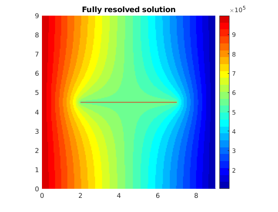
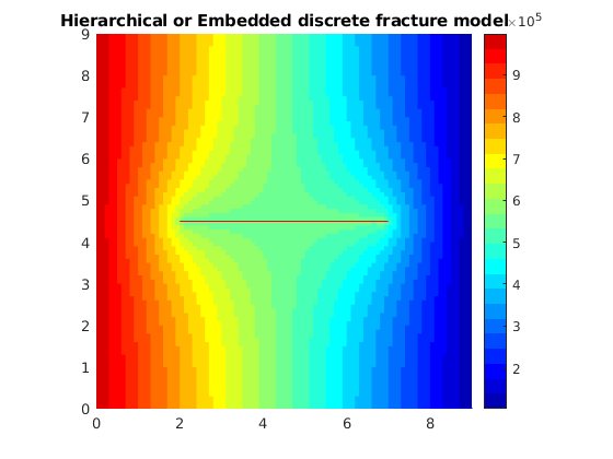
In this first introductory example to the HFM module, we consider a single-phase 2D example with Dirichlet boundary conditions and a horizontal central fracture in the centre. The example shows the effect of a single fracture on the reservoir pressure distribution. Moreover, the pressure solution obtained using an embedded discrete or hierarchical fracture model is compared to the results obtained from a fully resolved simulation where the fracture and matrix grid blocks are of the same size.
% Load necessary modules, etc
mrstModule add hfm;             % hybrid fracture module
mrstModule add incomp;          % Incompressible fluid models
checkLineSegmentIntersect;      % ensure lineSegmentIntersect.m is on path
Grid and fracture lines
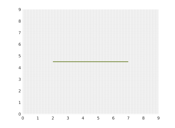
Construct a Cartesian grid comprising 90-by-90 cells, where each cell has dimension 0.1-by-0.1 m^2. Define a horizontal fracture line, 5 m in length, in the centre of the domain by supplying its end points (2, 4.5) and (7, 4.5) as a 1-by-4 array of the format [x1 y1 x2 y2].
celldim = [90 90];
physdim = [9 9];
G = cartGrid(celldim, physdim);
G = computeGeometry(G);

fl = [20, 45, 70, 45]./10 ; % fractures lines in [x1 y1 x2 y2] format.
Process fracture lines
Using the input fracture lines, we identify independent fracture networks comprising of connected lines. In this example, there is only 1 fracture network consisting of 1 fracture line. We also identify the fine-cells in the matrix containing these fractures. Fracture aperture is set to 0.04 meters. The matrix grid and fracture lines are plotted.
dispif(mrstVerbose, 'Processing user input...\n\n');
[G,fracture] = processFracture2D(G,fl);
fracture.aperture = 1/25; % Fracture aperture
figure;
plotFractureLines(G,fracture);
axis tight;
box on
Compute CI and construct fracture grid
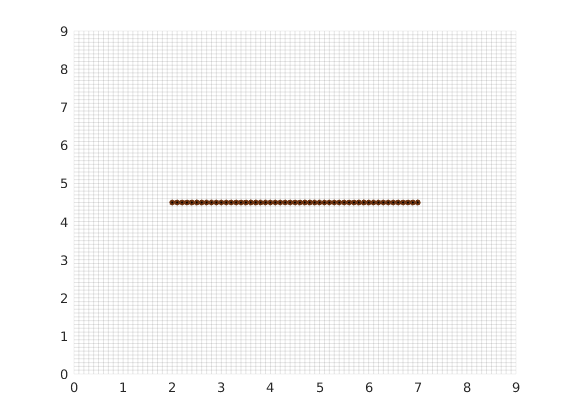
For each matrix block containing a fracture, we compute a fracture-matrix conductivity index (CI) in accordance with the hierarchical fracture model (a.k.a. embedded discrete fracture model). Following that, we compute a fracture grid where the fracture cell size is defined to be 0.1 m. Next, the fracture grid is plotted on top of the matrix grid.
dispif(mrstVerbose, 'Computing CI and constructing fracture grid...\n\n');
G = CIcalculator2D(G,fracture);
min_size = 0.05; cell_size = 0.1; % minimum and average cell size.
[G,F,fracture] = gridFracture2D(G,fracture,'min_size',min_size,'cell_size',cell_size);
clf; plotFractureNodes2D(G,F,fracture); box on
Set rock properties in fracture and matrix
Set the permeability (K) as 1 Darcy in the matrix and 10000 Darcy in the fractures.
dispif(mrstVerbose, 'Initializing rock and fluid properties...\n\n');
G.rock.perm = ones(G.cells.num,1) * darcy;
K_frac = 10000; % Darcy
G = makeRockFrac(G, K_frac);
Define fluid properties
Define a single fluid of viscosity 1 cP and density 1000 kg/m3.
fluid = initSingleFluid('mu', 1*centi*poise, 'rho', 1000*kilogram/meter^3);
Define fracture connections as NNC and compute the transmissibilities
In this section, we use the function defineNNCandTrans to combine the fracture and matrix grid structures into a single grid structure. In addition to that, we assign a ‘non-neighbouring connection (NNC)’ status to every fracture-matrix connection. For example, if fracture cell ‘i’ is located in the matrix cell ‘j’, then the connection i-j is defined as an NNC. To compute the flux between these elements, we compute a transmissibility for each NNC using the CI’s computed earlier. Vector T contains the transmissibility for each face in the combined grid and each NNC.
[G,T] = defineNNCandTrans(G,F,fracture);
Define completely resolved grid
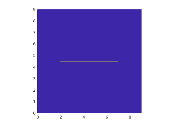
We now define the fully resolved grid where the matrix and fracture cells are of the same size. Rock properties for this new grid are defined such that a 5 m long horizontal line of cells in the centre of the domain has a permeability of 10000 Darcy whereas the rest of the grid has a permeability of 1 Darcy.
celldim = [225 225];
physdim = [9 9];
Gr = cartGrid(celldim, physdim);
Gr = computeGeometry(Gr);
Gr.rock.perm = ones(Gr.cells.num,1) * darcy;
fractureCells = 225*112+50:225*112+175;
Gr.rock.perm(fractureCells) = 10000*darcy;
clf; plotCellData(Gr,Gr.rock.perm,'EdgeColor', 'none'); axis equal tight
Initialize state variables
Here, we initialize the solution structure for the two grids.
dispif(mrstVerbose, 'Computing coefficient matrix...\n\n');
state  = initResSol (G, 5*barsa);
state_r  = initResSol (Gr, 5*barsa);
Add BC
Set boundary condition P = 10 bars on the left face and P = 1 bar on the right face of the domain.
bc = [];
bc  = pside(bc, G, 'LEFT', 10*barsa);
bc  = pside(bc, G, 'RIGHT', 1*barsa);

bcr = [];
bcr  = pside(bcr, Gr, 'LEFT', 10*barsa);
bcr  = pside(bcr, Gr, 'RIGHT', 1*barsa);
Compute pressure
The fine scale pressure solution is computed for both the grids using the boundary conditions provided and the transmissiblity matrix computed earlier.
dispif(mrstVerbose, '\nSolving fine-scale system...\n\n');
state = incompTPFA(state, G, T, fluid, 'bc', bc, 'use_trans',true);
state_r = incompTPFA(state_r, Gr, computeTrans(Gr,Gr.rock), fluid, 'bc', bcr);
Plot results
Use a reduced number of color levels to better compare and contrast the two solutions
figure
plotCellData(Gr, state_r.pressure,'EdgeColor','none')
line(fl(:,1:2:3)',fl(:,2:2:4)','Color','r','LineWidth',0.5);
colormap jet(25)
view(0, 90); colorbar; axis equal tight, cx = caxis();
title('Fully resolved solution')

figure
plotCellData(G, state.pressure,'EdgeColor','none')
line(fl(:,1:2:3)',fl(:,2:2:4)','Color','r','LineWidth',0.5);
colormap jet(25)
view(0, 90); colorbar; axis equal tight, caxis(cx);
title('Hierarchical or Embedded discrete fracture model');
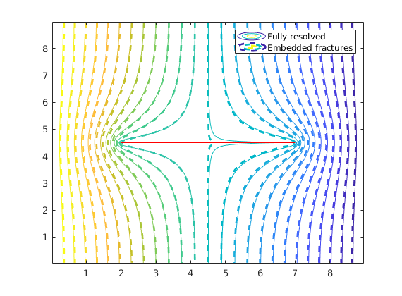
Add a contour plot
igure
contour(reshape(Gr.cells.centroids(:,1),Gr.cartDims),...
   reshape(Gr.cells.centroids(:,2),Gr.cartDims),...
   reshape(state_r.pressure,Gr.cartDims),25);
hold on
nc = prod(G.cartDims);
contour(reshape(G.cells.centroids(1:nc,1),G.cartDims),...
   reshape(G.cells.centroids(1:nc,2),G.cartDims),...
   reshape(state.pressure(1:nc),G.cartDims),25,'--','LineWidth',2);
line(fl(:,1:2:3)',fl(:,2:2:4)','Color','r','LineWidth',0.5);
hold off
legend('Fully resolved','Embedded fractures');

% <html>
% <p><font size="-1
Two-Phase Problem with a Quarter Five-Spot Well Pattern
Generated from fineScale2phWells.m
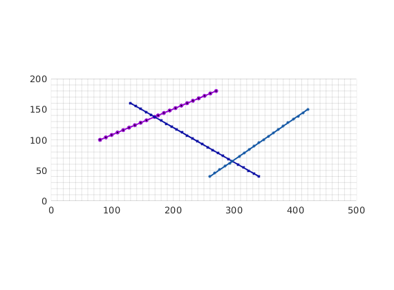
In this second introductory example to the HFM module, we show the impact of fractures on fluid migration using the hierarchical/embedded fracture model. To this end, we consider a two-phase example with three intersecting fractures in the center of the model. Oil is recovered by a production well in the NE corner, which is supported by a water-injector in the SW corner.
% Load necessary modules, etc
mrstModule add hfm;             % hybrid fracture module
mrstModule add mrst-gui;        % plotting routines
mrstModule add incomp;          % Incompressible fluid models
checkLineSegmentIntersect;      % ensure lineSegmentIntersect.m is on path
Grid and fracture lines
Construct a Cartesian grid comprising 50-by-20 cells, where each cell has dimension 10-by-10 m^2. Define 3 fracture lines by supplying their end points in the form [x1 y1 x2 y2].
celldim = [50 20];
physdim = [500 200];
G = cartGrid(celldim, physdim);
G = computeGeometry(G);

fl = [80,  100, 270, 180;...
      130, 160, 340,  40;...
      260,  40, 420, 150] ; % fractures lines in [x1 y1 x2 y2] format.
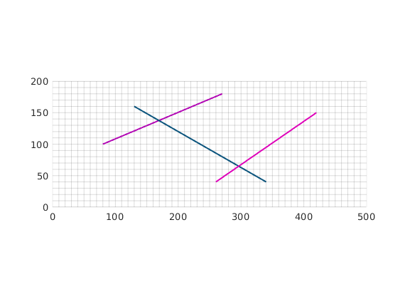
Process fracture lines
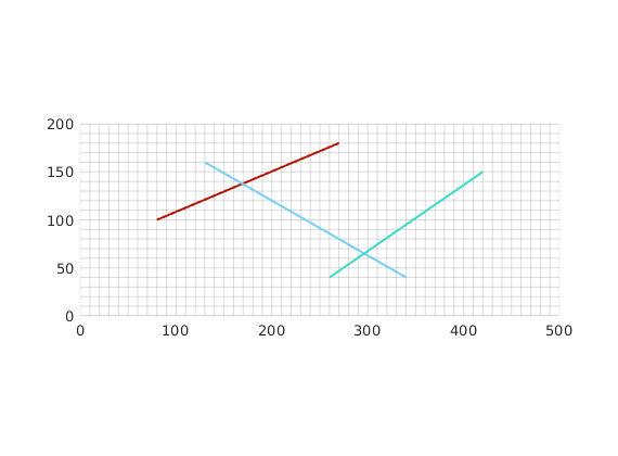
Using the input fracture lines, we identify independent fracture networks comprising of connected lines. In this example, there is only 1 fracture network consisting of 3 fracture lines. We also identify the fine-cells in the matrix containing these fractures. Fracture aperture is set to 0.04 meters. The matrix grid and fracture lines are plotted.
dispif(mrstVerbose, 'Processing user input...\n\n');
[G,fracture] = processFracture2D(G, fl, 'verbose', mrstVerbose);
fracture.aperture = 1/25; % Fracture aperture
figure;
plotFractureLines(G,fracture);
axis equal tight;
box on
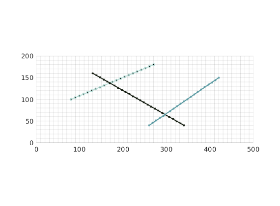
Compute CI and construct fracture grid
For each matrix block containing a fracture, we compute a fracture-matrix conductivity index (CI) in accordance with the hierarchical fracture model (a.k.a. embedded discrete fracture model). Following that, we compute a fracture grid where the fracture cell size is defined to be 10 m. Next, the fracture grid is plotted on top of the matrix grid.
dispif(mrstVerbose, 'Computing CI and constructing fracture grid...\n\n');
G = CIcalculator2D(G,fracture);
min_size = 5; cell_size = 10; % minimum and average cell size.
[G,F,fracture] = gridFracture2D(G,fracture,'min_size',min_size,'cell_size',cell_size);
clf; plotFractureNodes2D(G,F,fracture);
axis equal tight; box on
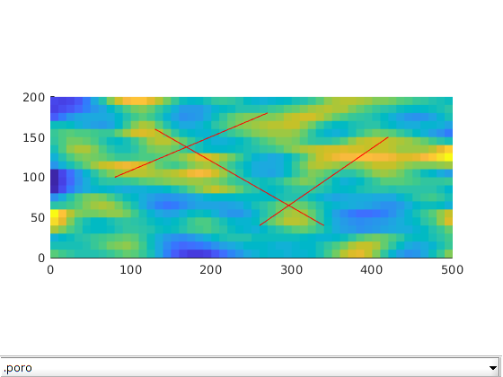
Set rock properties in fracture and matrix
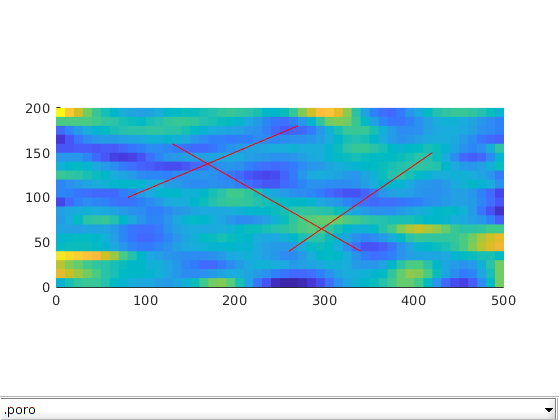
For this example, we will generate the porosity as a Gaussian field. To get a crude approximation to the permeability-porosity relationship, we assume that our medium is made up of uniform spherical grains of diameter dp = 10 m, for which the specic surface area is Av = 6 = dp. With these assumptions, using the Carman Kozeny relation, we can then calculate the isotropic permeability (K). The rock properties are then plotted.
dispif(mrstVerbose, 'Initializing rock and fluid properties...\n\n');
p = gaussianField(celldim, [0.2 0.4], [11 3], 2.5);
K = p.^3.*(1e-5)^2./(0.81*72*(1-p).^2);
G.rock.poro = p(:);
G.rock.perm = K(:);
K_frac = 10000; % Darcy
G = makeRockFrac(G, K_frac, 'porosity', 0.8);
clf; plotToolbar(G, G.rock); axis equal tight;
line(fl(:,1:2:3)',fl(:,2:2:4)',1e-3*ones(2,size(fl,1)),'Color','r','LineWidth',0.5);
Define fluid properties
Define a two-phase fluid model without capillarity. The fluid model has the values:
fluid = initSimpleFluid('mu' , [   1,  1] .* centi*poise     , ...
    'rho', [1000, 700] .* kilogram/meter^3, ...
    'n'  , [   2,   2]);
Define fracture connections as NNC and compute the transmissibilities
In this section, we use the function defineNNCandTrans to combine the fracture and matrix grid structures into a single grid structure. In addition to that, we assign a ‘non-neighbouring connection (NNC)’ status to every fracture-matrix connection. For example, if fracture cell ‘i’ is located in the matrix cell ‘j’, then the connection i-j is defined as an NNC. To compute the flux between these elements, we compute a transmissibility for each NNC using the CI’s computed earlier. Vector T contains the transmissibility for each face in the combined grid and each NNC.
[G,T] = defineNNCandTrans(G,F,fracture);
Add wells
We will include two wells, one rate-controlled injector well and the producer controlled by bottom-hole pressure. The injector and producer are located at the bottom left and top right corner of the grid, respectively. Wells are described using a Peaceman model, giving an extra set of equations that need to be assembled, see simpleWellExample.m for more details on the Peaceman well model.
inj = 1;
prod = celldim(1)*celldim(2);
wellRadius = 0.1;

W = addWell([], G.Matrix, G.Matrix.rock, inj,'InnerProduct', 'ip_tpf','Type', ...
    'rate', 'Val', 10, 'Radius', wellRadius, 'Comp_i', [1, 0]);
W = addWell(W, G.Matrix, G.Matrix.rock, prod, 'InnerProduct', 'ip_tpf', 'Type', ...
    'bhp' , 'Val', 50*barsa, 'Radius', wellRadius, 'Comp_i', [0, 1]);
Initialize state variables
Here, we initialize the solution structure using the combined grid and the wells defined above.
dispif(mrstVerbose, 'Computing coefficient matrix...\n\n');
state  = initResSol (G, 0);
state.wellSol = initWellSol(W, 0);
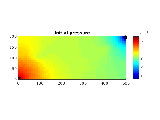
Compute initial pressure
dispif(mrstVerbose, '\nSolving fine-scale system...\n\n');
state = incompTPFA(state, G, T, fluid, 'Wells', W, 'MatrixOutput', true, 'use_trans',true);
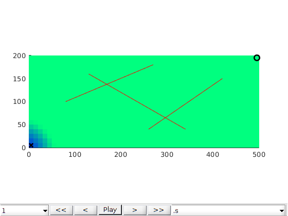
Plot initial pressure
clf
hp = plotCellData(G, state.pressure,'EdgeColor','none');
xw = G.cells.centroids(vertcat(W.cells),:);
hold on
plot3(xw(1,1),xw(1,2),1e-3,'xk','LineWidth',2,'MarkerSize',8);
plot3(xw(2,1),xw(2,2),1e-3,'ok','LineWidth',2,'MarkerSize',8);
hold off
colormap jet
view(0, 90); colorbar; axis equal tight;
title('Initial pressure');
Incompressible Two-Phase Flow
We solve the two-phase system using a sequential splitting in which the pressure and fluxes are computed by solving the flow equation and then held fixed as the saturation is advanced according to the transport equation. This procedure is repeated for a given number of time steps (here we use 60 equally spaced time steps amounting to 50 % PV Injected). The error introduced by this splitting of flow and transport can be reduced by iterating each time step until e.g., the residual is below a certain user-prescribed threshold (this is not done herein).
pv     = poreVolume(G,G.rock);
nt     = 60;
Time   = 0.5*(sum(pv)/state.wellSol(1).flux);
dT     = Time/nt;
dTplot = Time/3;
N      = fix(Time/dTplot);

pvi = zeros(nt,1);
sol = cell(nt,1);

t  = 0;
count = 1; title('Saturation');
colorbar off; colormap(flipud(winter));
while t < Time,
    state = implicitTransport(state, G, dT, G.rock, fluid, 'wells', W, 'Trans', T,'verbose',true);

    % Check for inconsistent saturations
    assert(max(state.s(:,1)) < 1+eps && min(state.s(:,1)) > -eps);

    % Plot saturation
    delete(hp)
    hp = plotCellData(G,state.s,state.s>0); drawnow; pause(.1);

    % Update solution of pressure equation.
    state  = incompTPFA(state, G, T, fluid, 'wells', W, 'use_trans',true);
    sol{count,1} = state;

    t = t + dT;
    pvi(count) = 100*(sum(state.wellSol(1).flux)*t)/sum(pv);
    count = count + 1;

end
implicitTransport:
----------------------------------------------------------------------
Time interval (s)     iter  relax   residual          rate
----------------------------------------------------------------------
 [0.0e+00, 2.3e+01]:   1    1.00    2.07848e+00              NaN
 [0.0e+00, 2.3e+01]:   2    0.25    1.17721e+00             0.42
 [0.0e+00, 2.3e+01]:   3    1.00    5.38623e-01             1.38
...
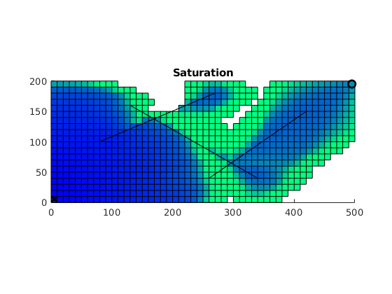
Plot saturations
lf, plotToolbar(G,cellfun(@(x) struct('s', x.s(:,1)), sol,'UniformOutput', false));
line(fl(:,1:2:3)',fl(:,2:2:4)',1e-3*ones(2,size(fl,1)),'Color','r','LineWidth',0.5);
hold on
plot3(xw(1,1),xw(1,2),1e-3,'xk','LineWidth',2,'MarkerSize',8);
plot3(xw(2,1),xw(2,2),1e-3,'ok','LineWidth',2,'MarkerSize',8);
hold off
colormap(flipud(winter)); caxis([0 1]); axis equal tight;

% <html>
% <p><font size="-1
Gas injection problem
Generated from fineScale3ph.m
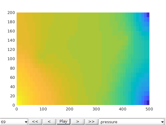
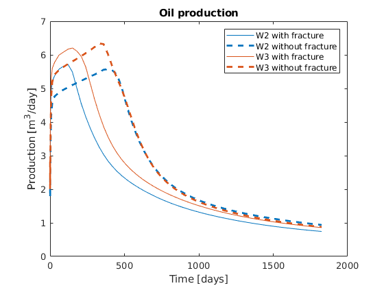
In this example, we consider the same setup as in the two-phase example with wells, except that we now assume a three-phase, compressible model with gas injection. For comparison, we also simulate injection in the same reservoir geometry without (embedded) fractures. The purpose of the example is to demonstrate how the methods from the HFM module easily can be combined with solvers from the ad-blackoil module.
% Load necessary modules, etc
mrstModule add hfm;             % hybrid fracture module
mrstModule add mrst-gui;        % plotting routines
mrstModule add ad-props ad-core % AD framework
mrstModule add ad-blackoil      % Three phase simulator
checkLineSegmentIntersect;      % ensure lineSegmentIntersect.m is on path
Grid and fracture lines
Construct a Cartesian grid comprising 50-by-20 cells, where each cell has dimension 10-by-10 m^2. Define 3 fracture lines by supplying their end points in the form [x1 y1 x2 y2].
celldim = [50 20];
physdim = [500 200];
G = cartGrid(celldim, physdim);
G = computeGeometry(G);

fl = [80,  100, 270, 180;...
      130, 160, 340,  40;...
      260,  40, 420, 150] ; % fractures lines in [x1 y1 x2 y2] format.
Process fracture lines
Using the input fracture lines, we identify independent fracture networks comprising of connected lines. In this example, there is only 1 fracture network consisting of 3 fracture lines. We also identify the fine-cells in the matrix containing these fractures. Fracture aperture is set to 0.04 meters. The matrix grid and fracture lines are plotted.
dispif(mrstVerbose, 'Processing user input...\n\n');
[G,fracture] = processFracture2D(G, fl, 'verbose', mrstVerbose);
fracture.aperture = 1/25; % Fracture aperture
figure;
plotFractureLines(G,fracture);
axis equal tight;
box on
Compute CI and construct fracture grid
For each matrix block containing a fracture, we compute a fracture-matrix conductivity index (CI) in accordance with the hierarchical fracture model (a.k.a. embedded discrete fracture model). Following that, we compute a fracture grid where the fracture cell size is defined to be 10 m. Next, the fracture grid is plotted on top of the matrix grid.
dispif(mrstVerbose, 'Computing CI and constructing fracture grid...\n\n');
G = CIcalculator2D(G,fracture);
min_size = 5; cell_size = 10; % minimum and average cell size.
[G,F,fracture] = gridFracture2D(G,fracture,'min_size',min_size,'cell_size',cell_size);
clf; plotFractureNodes2D(G,F,fracture);
axis equal tight; box on
Set rock properties in fracture and matrix
For this example, we will generate the porosity as a Gaussian field. To get a crude approximation to the permeability-porosity relationship, we assume that our medium is made up of uniform spherical grains of diameter dp = 10 m, for which the specic surface area is Av = 6 = dp. With these assumptions, we can then use the Carman Kozeny relation to calculate the isotropic permeability (K). The rock properties are then plotted. We also identify fracture-matrix and fracture-fracture connections and compute transmissibility for each connection.
dispif(mrstVerbose, 'Initializing rock and fluid properties...\n\n');
p = gaussianField(celldim, [0.2 0.4], [11 3], 2.5);
mp = 0.01;
p(p < mp) = mp;
K = p.^3.*(1e-5)^2./(0.81*72*(1-p).^2);

p = p(:);
K = K(:);

G.rock.poro = p(:);
G.rock.perm = K(:);
K_frac = 10000; % Darcy
G = makeRockFrac(G, K_frac, 'porosity', 0.8);

clf; plotToolbar(G, G.rock); axis tight equal
line(fl(:,1:2:3)',fl(:,2:2:4)',1e-3*ones(2,size(fl,1)),'Color','r','LineWidth',0.5);

[G,T] = defineNNCandTrans(G,F,fracture);
Define fluid properties
Define a two-phase fluid model without capillarity. The fluid model has the values:
fluid = initSimpleADIFluid('mu' , [   1,  5, 0.2] .* centi*poise     , ...
                           'rho', [1000, 700, 250] .* kilogram/meter^3, ...
                           'n'  , [   2,   2, 2]);

pRef = 100*barsa;
c_w = 1e-8/barsa;
c_o = 1e-5/barsa;
c_g = 1e-3/barsa;

fluid.bW = @(p) exp((p - pRef)*c_w);
fluid.bO = @(p) exp((p - pRef)*c_o);
fluid.bG = @(p) exp((p - pRef)*c_g);
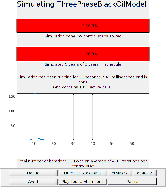
Define three-phase compressible flow model
We define a three-phase black-oil model without dissolved gas or vaporized oil. This is done by first instantiating the blackoil model, and then manually passing in the internal transmissibilities and the topological neighborship from the embedded fracture grid. This will cause a warning that can simply be ignored.
model = ThreePhaseBlackOilModel(G, [], fluid, 'disgas', false, 'vapoil', false);
N = getNeighbourship(G, 'topological', true);
intx = all(N ~= 0, 2);

% Send in internal transmissibility and neighborship to the operator setp

model.operators = setupOperatorsTPFA(G, G.rock, 'trans', T(intx), 'neighbors', N(intx, :));
Add wells
We have a single gas injector that injects a total of one pore volume of gas at surface conditions over a period of five years. Two producers are added and set to bottom hole pressure controls of 50 bar.
totTime = 5*year;
tpv = sum(model.operators.pv);

inj = 1;
prod1 = celldim(1)*celldim(2);
prod2 = celldim(1);
wellRadius = 0.1;

% Injector
W = addWell([], G.Matrix, G.Matrix.rock, inj,'InnerProduct', 'ip_tpf','Type', ...
    'rate', 'Val', tpv/totTime, 'Radius', wellRadius, 'Comp_i', [0, 0, 1]);
% First producer
W = addWell(W, G.Matrix, G.Matrix.rock, prod1, 'InnerProduct', 'ip_tpf', 'Type', ...
    'bhp' , 'Val', 50*barsa, 'Radius', wellRadius, 'Comp_i', [1, 1, 1]/3);
% Second producer
W = addWell(W, G.Matrix, G.Matrix.rock, prod2, 'InnerProduct', 'ip_tpf', 'Type', ...
    'bhp' , 'Val', 50*barsa, 'Radius', wellRadius, 'Comp_i', [1, 1, 1]/3);
Set up initial state and schedule
We set up a initial state with the reference pressure and a mixture of water and oil initially. We also set up a simple-time step strategy that ramps up gradually towards 30 day time-steps.
s0 = [0.2, 0.8, 0];
state  = initResSol(G, pRef, s0);
dt = rampupTimesteps(totTime, 30*day, 8);
schedule = simpleSchedule(dt, 'W', W);
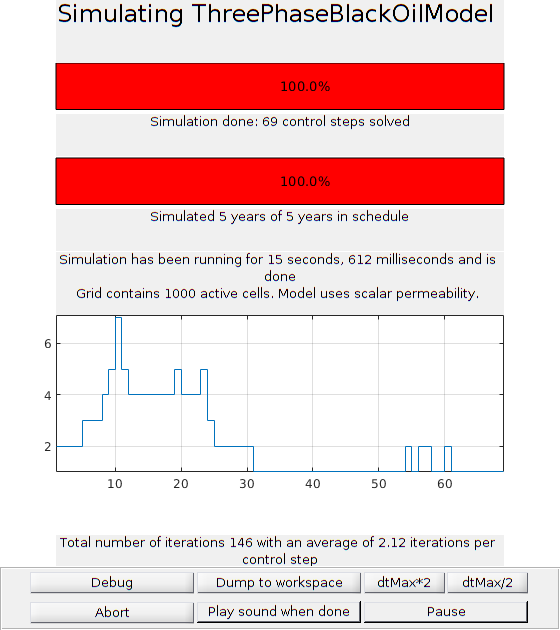
Simulate problem
%fn = getPlotAfterStep(state, model, schedule);
[ws, states, report] = simulateScheduleAD(state, model, schedule, ...
   'afterStepFn', getPlotAfterStep(state, model, schedule));
Solving timestep 01/69:         -> 2 Hours, 2925 Seconds
Solving timestep 02/69: 2 Hours, 2925 Seconds -> 5 Hours, 2250 Seconds
Solving timestep 03/69: 5 Hours, 2250 Seconds -> 11 Hours, 900 Seconds
Solving timestep 04/69: 11 Hours, 900 Seconds -> 22 Hours, 1800 Seconds
Solving timestep 05/69: 22 Hours, 1800 Seconds -> 1 Day, 21 Hours
Solving timestep 06/69: 1 Day, 21 Hours -> 3 Days, 18 Hours
Solving timestep 07/69: 3 Days, 18 Hours -> 7 Days, 12 Hours
Solving timestep 08/69: 7 Days, 12 Hours -> 15 Days
...
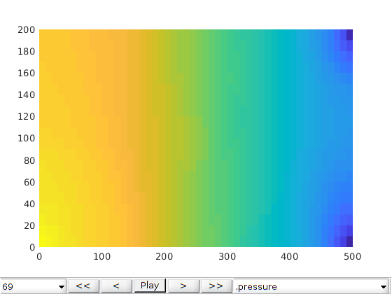
Create and solve the same problem without any fractures present
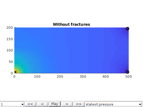
Fractures can have a large impact on fluid displacement, but are often associated with great uncertainty in terms of locations, orientation and permeability. To demonstrate the effect of fractures on the transport, we create another problem where the fractures themselves have been omitted.
G0 = cartGrid(celldim, physdim);
G0 = computeGeometry(G0);
% Create rock without fractures
rock0 = makeRock(G0, K, p);
% Same model, but different grid and rock
model0 = ThreePhaseBlackOilModel(G0, rock0, fluid, 'disgas', false, 'vapoil', false);
state0  = initResSol(G0, pRef, s0);

% Make a copy of the wells in the new grid
W0 = [];
for i = 1:numel(W)
    w = W(i);
    W0 = addWell(W0, G0, rock0, w.cells, 'type', w.type, 'val', w.val, ...
                 'wi', w.WI, 'comp_i', w.compi);
end
% Set up and simulate the schedule
schedule0 = simpleSchedule(dt, 'W', W0);
[ws0, states0, report0] = simulateScheduleAD(state0, model0, schedule0, ...
   'afterStepFn', getPlotAfterStep(state0, model0, schedule0));
Solving timestep 01/69:         -> 2 Hours, 2925 Seconds
Solving timestep 02/69: 2 Hours, 2925 Seconds -> 5 Hours, 2250 Seconds
Solving timestep 03/69: 5 Hours, 2250 Seconds -> 11 Hours, 900 Seconds
Solving timestep 04/69: 11 Hours, 900 Seconds -> 22 Hours, 1800 Seconds
Solving timestep 05/69: 22 Hours, 1800 Seconds -> 1 Day, 21 Hours
Solving timestep 06/69: 1 Day, 21 Hours -> 3 Days, 18 Hours
Solving timestep 07/69: 3 Days, 18 Hours -> 7 Days, 12 Hours
Solving timestep 08/69: 7 Days, 12 Hours -> 15 Days
...
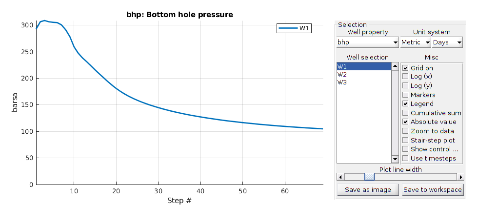
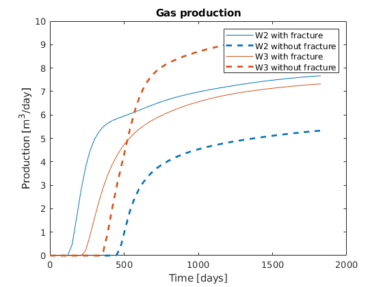
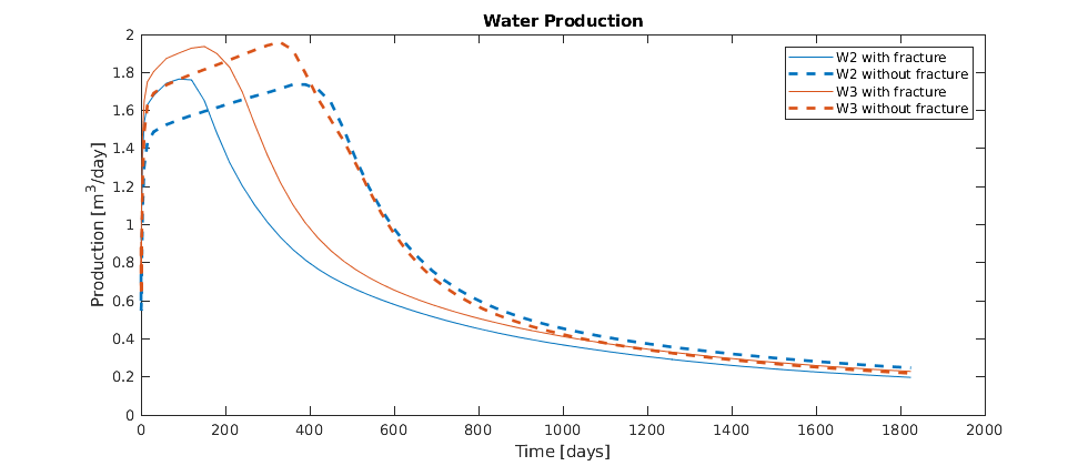
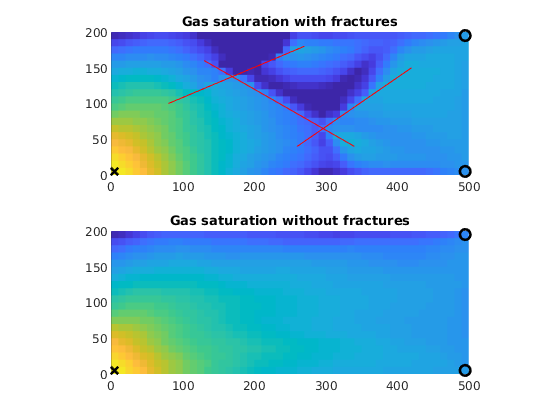
Plot the results
We plot the production curves for the two wells and compare between the two cases, as well as the final gas saturation.
tm = report.ReservoirTime/day;
flds = {'qGs', 'qWs', 'qOs'};
names = {'Gas production', 'Water Production', 'Oil production'};
sgn = vertcat(W.sign);
inj = find(sgn > 0);
prod = find(sgn <= 0);
colors = lines(nnz(prod));

for i = 1:numel(flds)
    figure(i); clf
    q0 = -getWellOutput(ws0, flds{i}, prod)*day;
    q =  -getWellOutput(ws, flds{i}, prod)*day;
    l = {};
    for j = 1:numel(prod)
        c = colors(j, :);

        plot(tm, q(:, j), 'color', c);
        hold on
        plot(tm, q0(:, j), '--', 'color', c, 'linewidth', 2);
        title(names{i})
        ylabel('Production [m^3/day]');
        xlabel('Time [days]')
        n = W(prod(j)).name;
        l = [l, {[n, ' with fracture'], [n, ' without fracture']}]; %#ok
    end
    legend(l)
end

figure;
subplot(2, 1, 1)
plotCellData(G0, states{end}.s(1:G0.cells.num, 3), 'EdgeColor', 'none')
line(fl(:,1:2:3)',fl(:,2:2:4)',1e-3*ones(2,size(fl,1)),'Color','r','LineWidth',0.5);
axis equal tight
caxis([0, 1])
title('Gas saturation with fractures')
subplot(2, 1, 2)
plotCellData(G0, states0{end}.s(1:G0.cells.num, 3), 'EdgeColor', 'none')
title('Gas saturation without fractures')
axis equal tight
caxis([0, 1])
xw = G.cells.centroids(vertcat(W.cells),:);
for i=1:2,
   subplot(2,1,i)
   hold on
   plot3(xw(1,1),xw(1,2),1e-3,'xk','LineWidth',2,'MarkerSize',8);
   plot3(xw(2,1),xw(2,2),1e-3,'ok','LineWidth',2,'MarkerSize',8);
   plot3(xw(3,1),xw(3,2),1e-3,'ok','LineWidth',2,'MarkerSize',8);
   hold off
end
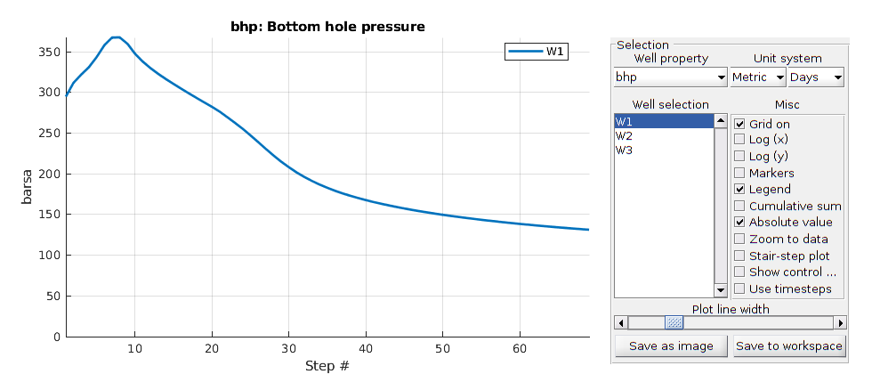
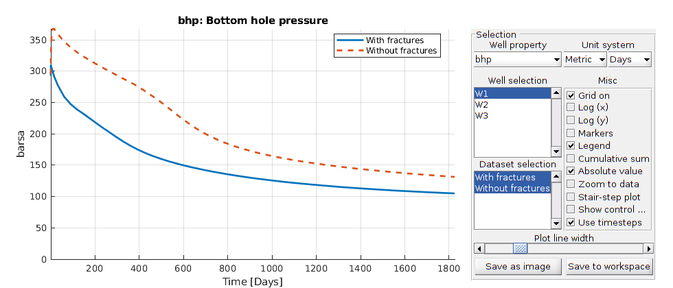
Interactive plotting
Compare the well cruves
lotWellSols({ws, ws0}, report.ReservoirTime, 'datasetnames', {'With fractures', 'Without fractures'})
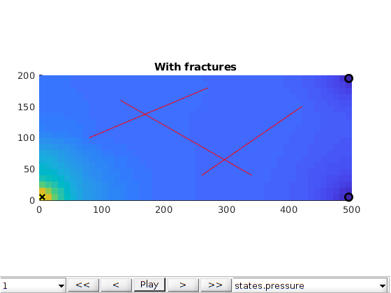
figure;
plotToolbar(G, states)
line(fl(:,1:2:3)',fl(:,2:2:4)',1e-3*ones(2,size(fl,1)),'Color','r','LineWidth',0.5);
hold on
plot3(xw(1,1),xw(1,2),1e-3,'xk','LineWidth',2,'MarkerSize',8);
plot3(xw(2,1),xw(2,2),1e-3,'ok','LineWidth',2,'MarkerSize',8);
plot3(xw(3,1),xw(3,2),1e-3,'ok','LineWidth',2,'MarkerSize',8);
hold off
axis equal tight
title('With fractures')
figure;
plotToolbar(G0, states0)
hold on
plot3(xw(1,1),xw(1,2),1e-3,'xk','LineWidth',2,'MarkerSize',8);
plot3(xw(2,1),xw(2,2),1e-3,'ok','LineWidth',2,'MarkerSize',8);
plot3(xw(3,1),xw(3,2),1e-3,'ok','LineWidth',2,'MarkerSize',8);
hold off
axis equal tight
title('Without fractures')
% <html>
% <p><font size="-1
Water injection into a 3D fractured porous media
Generated from simple2phHorizontalWell3D.m
Two-phase example with a horizontal producer and injector simulating water injection in a 3-dimensional fractured porous media using the HFM module. Note that the 3D solvers are not capable of handling intersecting fracture planes.
% Load necessary modules, etc
mrstModule add hfm;             % hybrid fracture module
mrstModule add coarsegrid;      % functionality for coarse grids
mrstModule add ad-core;         % NNC support for coarse grids
mrstModule add msrsb;           % MsRSB solvers
mrstModule add mrst-gui;        % plotting routines
mrstModule add incomp;          % Incompressible fluid models
checkMATLABversionHFM;
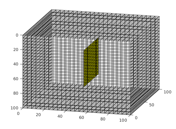
Grid and fracture(s)
Construct a Cartesian grid comprising 25-by-25-by-25 cells, where each cell has dimension 4-by-4-by-4 m^3. Define a fracture plane using a coplanar set of points supplied as rows in the matrix [X Y Z]. In this example, we define a fracture plane of size 50-by-50 m^2, extending in the y-direction through the centre of the domain. Fracture aperture is set to 0.02 meters. Additionally, we compute a triangulation using the matrix grid nodes. The triangulation is used to locate cells penetrated by the fracture plane in the next section.
celldim = [25, 25, 25];
physdim = [100 100 100];
G = cartGrid(celldim, physdim);
G = computeGeometry(G);
GlobTri = globalTriangulation(G);
fracplanes = struct;
fracplanes(1).points = [50 25 25;
                        50 25 75;
                        50 75 75;
                        50 75 25];
fracplanes(1).aperture = 1/50;
checkIfCoplanar(fracplanes)
Process fracture(s)
Using the input fracture, we identify fine-cells in the matrix containing these fractures. Next, a global conductivity index (CI) is computed for the fracture plane and a grid is defined over it. A ‘non-neighboring connection (NNC)’ status is given to each fracture-matrix connection and we compute the transmissibility for each NNC using the global CI.
dispif(mrstVerbose, 'Processing user input...\n\n');
[G,fracplanes] = preProcessingFractures(G, fracplanes, ...
                 'GlobTri', GlobTri, ...
                 'fractureCellSize', 0.3);
fprintf('\nProcessing complete...\n');

figure; plotGrid(G,'facealpha',0);
for i = 1:numel(fieldnames(G.FracGrid))
    plotGrid(G.FracGrid.(['Frac',num2str(i)]));
end
view(15,20);
Processing complete...
Set rock properties in fracture and matrix
Set the permeability (K) as 1 Darcy in the matrix and 10000 Darcy in the fractures. Additionally, set the porosity of the matrix and fractures to 20% and 50%, respectively.
dispif(mrstVerbose, 'Initializing rock and fluid properties...\n\n');
G.rock.perm = ones(G.cells.num,1)*darcy();
G.rock.poro = 0.2*ones(G.cells.num, 1);
K_frac = 10000; % Darcy
poro_frac = 0.5;
G = makeRockFrac(G, K_frac, 'permtype','homogeneous','porosity', poro_frac);
Define fluid properties
Define a two-phase fluid model without capillarity. The fluid model has the values:
fluid = initSimpleFluid('mu' , [   1,  1] .* centi*poise     , ...
    'rho', [1000, 700] .* kilogram/meter^3, ...
    'n'  , [   2,   2]);
Assemble global grid and compute transmissibilities
In this section, we combine the fracture and matrix grids into one grid. The transmissibility for each face in the combined grid and each NNC is computed and stored in the vector T.
G = assembleGlobalGrid(G);
G = computeEffectiveTrans(G);
G.faces.tag = zeros(G.faces.num,1);
x = ismember(G.faces.neighbors,G.nnc.cells,'rows');
G.faces.tag(x) = 1; % Tag NNC faces.
%
T = computeTrans(G, G.rock);
cf = G.cells.faces(:,1);
nf = G.faces.num;
T  = 1 ./ accumarray(cf, 1./T, [nf, 1]);
T = [T;G.nnc.T];
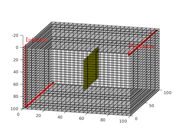
Add wells
We will include two horizontal wells, a rate-controlled injector well through the bottom left corner of the grid and a producer, controlled by bottom-hole pressure, through the top right section of the grid. Wells are described using a Peaceman model, giving an extra set of equations that need to be assembled, see simpleWellExample.m for more details on the Peaceman well model.
[nx, ny, nz] = deal(G.cartDims(1), G.cartDims(2), G.cartDims(3));
cellinj = nx*ny*(nz-1)+1:nx:nx*ny*nz;
cellprod = nx:nx:nx*ny;
W   = addWell([], G.Matrix, G.Matrix.rock, flipud(cellinj), 'Type', 'rate',...
    'Val', 500/day, 'Sign',1, 'Comp_i', [1, 0], 'Name', 'Injector');
W   = addWell(W, G.Matrix, G.Matrix.rock, cellprod, 'Type', 'bhp', ...
    'Val', 100*barsa, 'Sign', -1, 'Comp_i', [0, 1], 'Name', 'Producer');
plotWell(G,W);
Initialize state variables
Once the transmissibilities are computed, we can generate the transmissiblity matrix ‘A’ using the ‘two-point flux approximation’ scheme and initialize the solution structure.
dispif(mrstVerbose, 'Computing coefficient matrix...\n\n');
state  = initResSol (G, 0);
state.wellSol = initWellSol(W, 0);
[A,q] = getSystemIncompTPFA(state, G, T, fluid, 'use_trans', true);
Setup multiscale grids
Next, we define a 5-by-5-by-5 matrix coarse grid such that each coarse block contains 5-by-5-by-5 fine cells. The fracture plane is partitioned into 3-by-4 coarse blocks leading to a coarsening ratio of around 30. Additionally, we also define the support regions for the fracture and matrix basis functions. Fracture support region is defined based on a topological distance based algorithm. The matrix and fracture coarse grids are plotted in the next section.
nw = struct;
for i = 1:numel(fracplanes)
    nw(i).lines = i;
end

% Partition matrix
coarseDims = [5 5 5];
pm = partitionMatrix(G, 'coarseDims', coarseDims, 'use_metis', false);
CGm = getRsbGridsMatrix(G, pm, 'Wells', W);

% Partition fracture
coarseDimsF = [3 4];
p  = partitionFracture(G, pm, nw, 'partition_frac'   , true   , ...
    'use_metisF'       , false  , ...
    'coarseDimsF'      , coarseDimsF );

% p = processPartition(G,compressPartition(p));
pf = p(G.Matrix.cells.num+1:end)-max(p(1:G.Matrix.cells.num));

% Coarse Grids
CG = generateCoarseGrid(G, p);

% Add centroids / geometry information on coarse grid
CG = coarsenGeometry(CG);
Gf = assembleFracGrid(G);
CGf = generateCoarseGrid(Gf, pf);
CGf = coarsenGeometry(CGf);

% Support Regions
[CG,CGf] = storeFractureInteractionRegion(CG, CGf, CGm, ...
    'excludeBoundary' , false , ...
    'removeCenters'   , false , ...
    'fullyCoupled'    , false );
Compute initial pressure
dispif(mrstVerbose, '\nSolving fine-scale system...\n\n');
state_fs = incompTPFA(state, G, T, fluid,  ...
    'Wells', W, 'MatrixOutput', true, 'use_trans',true);
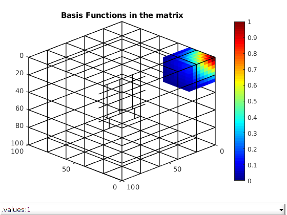
Compute basis functions
Using the transmissibility matrix ‘A’ we compute the basis functions for each fracture and matrix coarse block using the restriction smoothed basis method. Note that the matrix ‘A’ does not contain any source terms or boundary conditions. They are added to the coarse linear system when computing the multiscale pressure in the next section.
dispif(mrstVerbose, 'Computing basis functions...\n\n');
basis_sb = getMultiscaleBasis(CG, A, 'type', 'msrsb');
clf; plotToolbar(G,basis_sb.B,'filterzero',true); view(-135,30)
plotGrid(CG,'FaceColor','none','LineWidth',1);
axis tight; colormap(jet); colorbar;
title('Basis Functions in the matrix');
Compute multiscale solution
dispif(mrstVerbose, 'Computing multiscale solution...\n\n');
[state_ms,~] = incompMultiscale(state, CG, T, fluid, basis_sb,...
    'Wells', W,'use_trans',true);
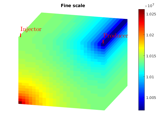
Plot initial pressure
figure;
plotToolbar(G, state_fs.pressure); plotWell(G,W);
colormap jet; colorbar
view(15,20)
axis tight off
title('Fine scale')
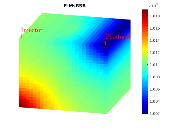
figure;
plotToolbar(G, state_ms.pressure); plotWell(G,W);
colormap jet; colorbar
view(15,20)
axis tight off
title('F-MsRSB')
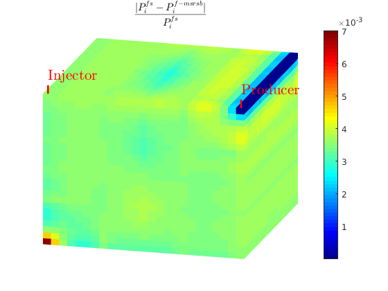
L1 = abs(state_ms.pressure-state_fs.pressure)./state_fs.pressure;
figure;
plotToolbar(G, L1)
plotWell(G,W); view(15,20);
colormap jet; colorbar
axis tight off
L1_eq = '$$ \frac{| P_i^{fs}-P_i^{f-msrsb} | }{ P_i^{fs} } $$';
title(L1_eq,'interpreter','latex');
Incompressible Two-Phase Flow
We solve the two-phase system using a sequential splitting in which the pressure and fluxes are computed by solving the flow equation and then held fixed as the saturation is advanced according to the transport equation. Note that the flow equations are solved in the fine scale as well as on the coarse scale using an algebraic multiscale strategy. The multiscale flux field obtained at fine scale resolution is reconstructed to be conservative before solving the transport equation. This procedure is repeated for a given number of time steps (here we use 30 equally spaced time steps amounting to 90 % PV Injected). The error introduced by this splitting of flow and transport can be reduced by iterating each time step until e.g., the residual is below a certain user-prescribed threshold (this is not done herein).
pv     = poreVolume(G,G.rock);
nt     = 30;
Time   = 0.9*(sum(pv)/abs(sum(state_fs.wellSol(1).flux)));
dT     = Time/nt;

pvi = zeros(nt,1);
sol_fs = cell(nt,1); sol_ms = cell(nt,1);
e = zeros(nt,1);

% Prepare plotting
clf, set(gcf,'Position',[0 0 980 400]); colormap(flipud(winter));
txt = {'Reference','F-MsRSB'};
for i=1:2, subplot(1,2,i),
   plotGrid(cartGrid([1 1 1],physdim), 'FaceColor','none','EdgeColor','k','LineWidth',1);
   plotWell(G,W); axis tight; view(20,15); title(txt{i});
end
[hfs,hms]=deal([]);

t  = 0;
B = basis_sb.B;
R = controlVolumeRestriction(CG.partition);
count = 1;
hwb = waitbar(0,'Time loop');
while t < Time,
    state_fs = implicitTransport(state_fs, G, dT, G.rock, fluid, 'wells', W, 'Trans', T,'verbose',true);
    state_ms = implicitTransport(state_ms, G, dT, G.rock, fluid, 'wells', W, 'Trans', T);
    % Check for inconsistent saturations
    s = [state_fs.s(:,1); state_ms.s(:,1)];
    assert(max(s) < 1+eps && min(s) > -eps);

    % Plot solution
    subplot(1,2,1); delete(hfs);
    hfs = plotCellData(G, state_fs.s(:,1),state_fs.s(:,1)>1e-3);
    subplot(1,2,2); delete(hms);
    hms = plotCellData(G, state_fs.s(:,1),state_ms.s(:,1)>1e-3);

    % Update solution of pressure equation.
    state_fs  = incompTPFA(state_fs , G, T, fluid, 'wells', W, 'use_trans',true);

    %-------------------------------Multiscale----------------------------%
    A = getSystemIncompTPFA(state_ms, G, T, fluid, 'use_trans', true);
    B = iteratedJacobiBasis(A, CG, 'interpolator', basis_sb.B);
    basis_sb = struct('B', B, 'R', R);
    state_ms = incompMultiscale(state_ms, CG, T, fluid, basis_sb, 'Wells', W,...
        'use_trans',true);
    %---------------------------------------------------------------------%

    sol_fs{count,1} = state_fs; sol_ms{count,1} = state_ms;
    % Increase time
    t = t + dT;
    waitbar(t/Time, hwb);
    pvi(count) = 100*(sum(state_fs.wellSol(1).flux)*t)/sum(pv);
    e(count,1) = sum(abs(state_fs.s(:,1) - state_ms.s(:,1)).*pv)/sum(pv.*state_fs.s(:,1));

    fprintf([num2str(pvi(count)), '%% PV injected \n']);
    count = count + 1;
end
close(hwb);
implicitTransport:
----------------------------------------------------------------------
Time interval (s)     iter  relax   residual          rate
----------------------------------------------------------------------
 [0.0e+00, 1.0e+06]:   1    1.00    2.45433e+00              NaN
 [0.0e+00, 1.0e+06]:   2    0.25    1.40030e+00             0.28
 [0.0e+00, 1.0e+06]:   3    0.50    6.43549e-01             1.39
...
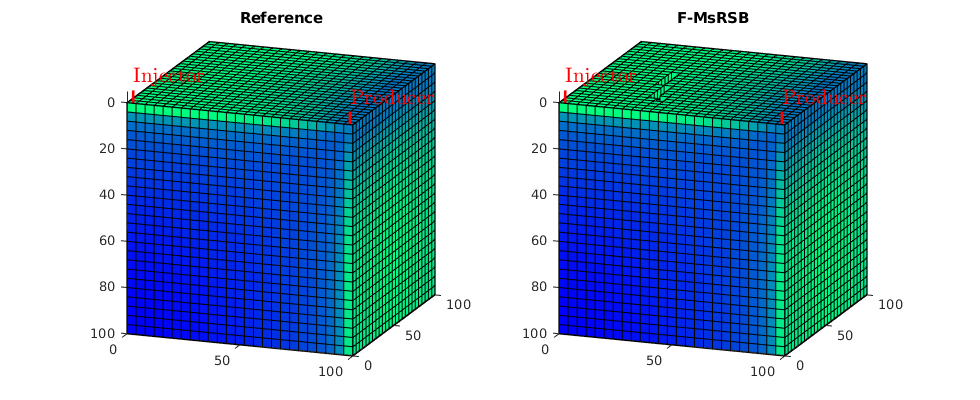
Plot saturations
To better see the evolution of the saturation front, you should change the patch properties (click the colored triangle in the bottom row of the menu) and set the faces to be semi-transparent (e.g., a value .5 to .7)
figure; plotToolbar(G,sol_fs); colormap(flipud(winter)); plotWell(G,W); view(15,20);
figure; plotToolbar(G,sol_ms); colormap(flipud(winter)); plotWell(G,W); view(15,20)

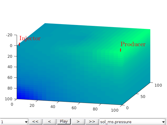
Plot error in saturation
igure;
plot(pvi,e*100, '--+b');
ylabel('e [%]')
xlabel('PVI [%]');
set(gca,'XGrid','on','YGrid','on');
axis tight

e_eq = '$$ e = \frac{ \sum ( |S_w^{fs}-S_w^{f-msrsb}| \times pv) }{ \sum (S_w^{fs} \times pv) } $$';
title(e_eq,'interpreter','latex');

% <html>
% <p><font size="-1
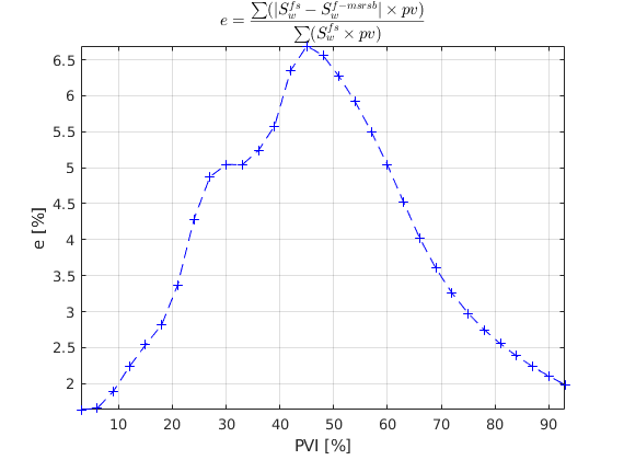
Water injection into a 3D fractured porous media
Generated from blackoil3D.m
Two-phase example with vertical producer/injector pair simulating water injection in a 3-dimensional fractured porous media using the EDFM method
Load necessary modules
mrstModule add hfm;             % hybrid fracture module
mrstModule add mrst-gui;        % plotting routines
mrstModule add ad-blackoil;     % AD blackoil solver
mrstModule add ad-core;         % AD core module
mrstModule add ad-props;        % AD properties
Set up a matrix grid
We first set up a Cartesian matrix grid with dimensions 500m x 200m x 100m with grid blocks that are 10m x 10m x 10m. Matrix permeability is 100mD and porosity is 30%.
celldim = [50, 20, 10];
physdim = [500, 200, 100];
G = cartGrid(celldim, physdim);
G = computeGeometry(G);
G.rock=makeRock(G,100*milli*darcy,0.3);

% Plot Matrix Grid
figure;
plotGrid(G,'facealpha',0,'edgealpha',0.5);
view(30,45);
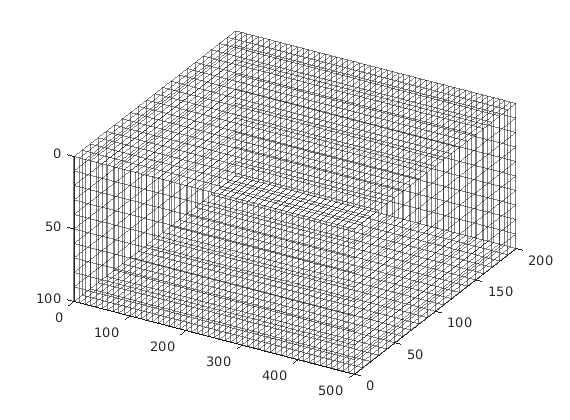
Set up fracture planes
Fracture planes are set up by defining their vertices. Additionally, the aperture, porosity and permeability of the fractures are provided. Fracture planes 1 and 3 will be vertical while fracture 2 is slanted.
% Fracture plane 1
fracplanes(1).points = [90 100 0;
                        140 160 0;
                        140 160 100;
                        90 100 100];
fracplanes(1).aperture = 1/25;
fracplanes(1).poro=0.8;
fracplanes(1).perm=10000*darcy;

% Fracture plane 2
points = [130 160 0
          340 40 0
          340 40 100
          130 160 100];

f2normal = getnormal(points);
points([1,2],:)=points([1,2],:)+f2normal*5; % displace top points
points([3,4],:)=points([3,4],:)-f2normal*5; % displace bottom points

fracplanes(2).points = points;
fracplanes(2).aperture = 1/25;
fracplanes(2).poro=0.8;
fracplanes(2).perm=10000*darcy;

% Fracture plane 3
fracplanes(3).points = [250 70 0
                        330 160 0
                        330 160 100
                        250 70 100];
fracplanes(3).aperture = 1/25;
fracplanes(3).poro=0.8;
fracplanes(3).perm=10000*darcy;

% Plot fracture planes
figure;
plotfracongrid(G,fracplanes); % visualize to check before pre-process
view(30,45)
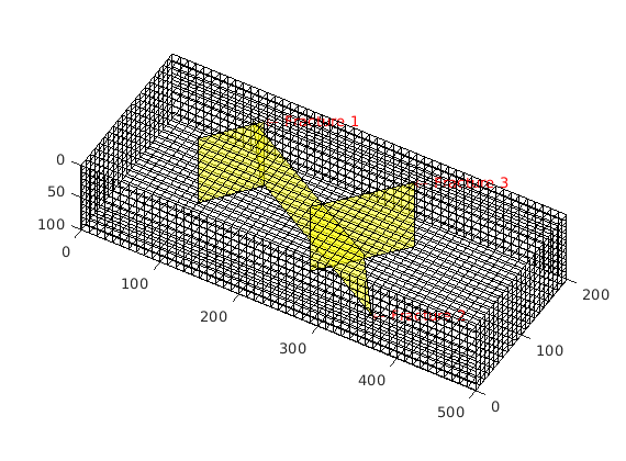
Construct fracture grid
The fracture grid is constructed using the matrix grid. The matrix grid will serve as a ‘cookie cutter’ to subdivide the fracture planes. Parallel processing can be used to speed up this process (Start a parallel pool to do this).
tol=1e-5;
[G,fracplanes]=EDFMgrid(G,fracplanes,...
    'Tolerance',tol,'fracturelist',1:3);

% Plot Fracture grid
figure;
plotGrid(cartGrid([1 1 1],physdim),'facealpha',0);
hold on;
plotGrid(G,G.Matrix.cells.num+1:G.cells.num);
axis tight equal
title('Fracture Grid')
view(30,45);
Processing 1 out of 3 fractures.
Processing 2 out of 3 fractures.
Processing 3 out of 3 fractures.
EDFM grid assembly took 4.3746 seconds.
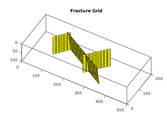
Fracture-Matrix non-Neighbouring Connections (NNC)
This calculates the transmissibilities between connected matrix and fracture grid blocks. Information is saved under G.nnc.
tol=1e-5;
G=fracturematrixNNC3D(G,tol);

% Plot matrix gridblocks that have NNCs with fractures
figure;
plotfracongrid(cartGrid([1 1 1],physdim),fracplanes);
hold on;
plotGrid(G,G.nnc.cells(:,1),'facealpha',0,'edgealpha',1);
axis tight equal
title('Matrix-Fracture NNCs')
view(30,45);
Processing Fracture-Matrix NNCs...
Processing Frac1...
Processing Frac2...
Processing Frac3...
Processing Fracture-Matrix NNCs completed in 6.8725 seconds!
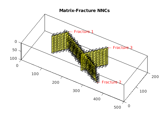
Fracture-Fracture NNCs
This calculates the transmissibilities between connected fracture and fracture grid blocks. Information is saved under G.nnc.
tol=1e-5;
[G,fracplanes]=fracturefractureNNCs3D(G,fracplanes,tol,'Verbose',true);

% Plot fracture gridblocks that have Fracture-Fracture NNCs
fraccells = G.nnc.cells(strcmp(G.nnc.type,'fracfrac'),:);
figure;
plotGrid(cartGrid([1 1 1],physdim),'facealpha',0);
hold on;
plotGrid(G,G.Matrix.cells.num+1:G.cells.num,'facealpha',0,'edgealpha',0.5);
plotGrid(G,fraccells);
axis equal tight;
title('Fracture-Fracture NNCs')
view(30,45);
Processing Fracture-Fracture NNCs...
Checking Frac1 vs Frac2.
Checking Frac1 vs Frac3.
Checking Frac2 vs Frac3.
Processing Fracture-Fracture NNCs completed in 2.2737 seconds!
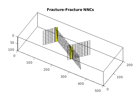
Setup TPFA Operators
Generate operators for the black oil model which incorporates all the NNCs identified above.
TPFAoperators = setupEDFMOperatorsTPFA(G, G.rock, tol);
Define fluid properties
Define a three-phase fluid model without capillarity.
fluid = initSimpleADIFluid('mu' , [   1,  5, 0.2] .* centi*poise     , ...
                           'rho', [1000, 700, 250] .* kilogram/meter^3, ...
                           'n'  , [   2,   2, 2]);

% Add compressibility to fluid
pRef = 100*barsa;
c_w = 1e-8/barsa;
c_o = 1e-5/barsa;
c_g = 1e-3/barsa;

fluid.bW = @(p) exp((p - pRef)*c_w);
fluid.bO = @(p) exp((p - pRef)*c_o);
fluid.bG = @(p) exp((p - pRef)*c_g);
Define three-phase compressible flow model
We define a three-phase black-oil model without dissolved gas or vaporized oil. This is done by first instantiating the blackoil model, and then manually passing in the internal transmissibilities and the topological neighborship from the embedded fracture grid.
gravity reset off
model = ThreePhaseBlackOilModel(G, [], fluid, 'disgas', false, 'vapoil', false);
model.operators = TPFAoperators;
Add wells
An injector/producer pair is added. 1PV of water is injected over the course of 5 years.
totTime = 5*year;
tpv = sum(model.operators.pv);
wellRadius = 0.1;
[nx, ny, nz] = deal(G.cartDims(1), G.cartDims(2), G.cartDims(3));

% Injector
cellinj = 1:nx*ny:(1+(nz-1)*nx*ny);
W   = addWell([], G.Matrix, G.Matrix.rock, cellinj,'InnerProduct', 'ip_tpf','Type', ...
    'rate', 'Val', tpv/totTime, 'Radius', wellRadius, 'Comp_i', [1, 0, 0], 'Name', 'Injector');

% Producer
cellprod = nx*ny:nx*ny:nz*nx*ny;
W   = addWell(W, G.Matrix, G.Matrix.rock, cellprod, 'InnerProduct', 'ip_tpf', 'Type', ...
    'bhp' , 'Val', 50*barsa, 'Radius', wellRadius, 'Comp_i', [1, 1, 0], 'Name', 'Producer');

% Plot setup
plotEDFMgrid(G);
hold on;
plotWell(G,W);
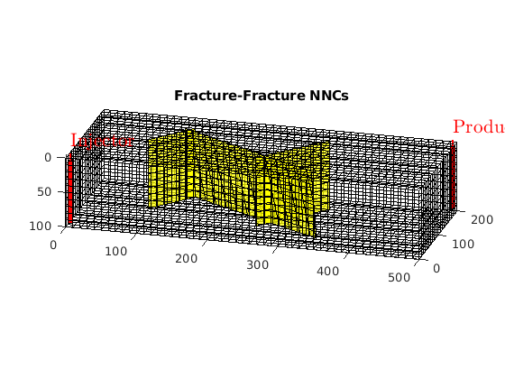
Set up initial state and schedule
We set up a initial state with the reference pressure and a mixture of water and oil initially. We also set up a simple-time step strategy that ramps up gradually towards 30 day time-steps.
s0 = [0.2, 0.8, 0];
state  = initResSol(G, pRef, s0);
dt = rampupTimesteps(totTime, 30*day, 8);
schedule = simpleSchedule(dt, 'W', W);
Simulate problem
[ws, states, report] = simulateScheduleAD(state, model, schedule, ...
   'afterStepFn', getPlotAfterStep(state, model, schedule));
Solving timestep 01/69:         -> 2 Hours, 2925 Seconds
Solving timestep 02/69: 2 Hours, 2925 Seconds -> 5 Hours, 2250 Seconds
Solving timestep 03/69: 5 Hours, 2250 Seconds -> 11 Hours, 900 Seconds
Solving timestep 04/69: 11 Hours, 900 Seconds -> 22 Hours, 1800 Seconds
Solving timestep 05/69: 22 Hours, 1800 Seconds -> 1 Day, 21 Hours
Solving timestep 06/69: 1 Day, 21 Hours -> 3 Days, 18 Hours
Solving timestep 07/69: 3 Days, 18 Hours -> 7 Days, 12 Hours
Solving timestep 08/69: 7 Days, 12 Hours -> 15 Days
...
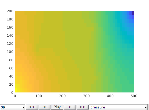
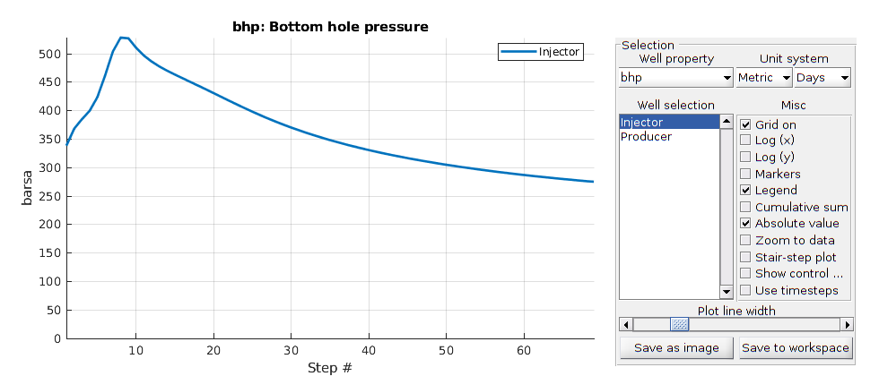
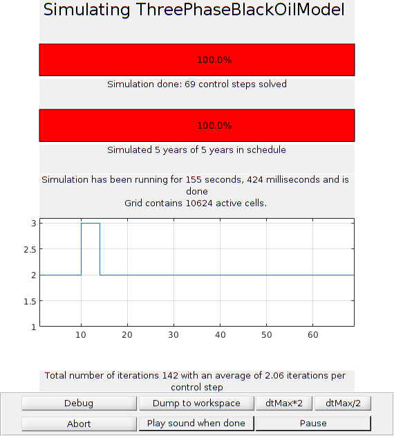
Single phase 2.5D problem
Generated from simpleExtruded.m
The matrix and fractures are represented in 3D by extruding their corresponding 2D grids.
% Load necessary modules, etc
mrstModule add hfm;             % hybrid fracture module
mrstModule add coarsegrid;      % functionality for coarse grids
mrstModule add ad-core;         % NNC support for coarse grids
mrstModule add msrsb;           % MsRSB solvers
mrstModule add mrst-gui;        % plotting routines
mrstModule add incomp;          % Incompressible fluid models
checkLineSegmentIntersect;      % ensure lineSegmentIntersect.m is on path
Grid and fracture lines
We start by constructing a 2D Cartesian grid comprising 50-by-50 cells, where each cell has dimension 1-by-1 m^2. Next, define 2 fracture lines in the form of a ‘x’ through the centre of the domain. We also define the number of layers in the extruded 3D grid and the indices of layers through which the fracture grid would extend. In this example, we extrude the matrix grid by 50 layers resulting in 50-by-50-by-50 fine cells. The fracture grid is extruded from layer 11 through 40.
celldim = [50 50];
G = cartGrid(celldim);
G = computeGeometry(G);
fl = [5 5 45 45; 5 45 45 5];
layers = 50;
flayers = 11:40;
Process fracture lines
Using the input fracture lines, we identify independent fracture networks comprising of connected lines. In this example, there is only 1 fracture network consisting of 2 fracture lines. We also identify the fine-cells in the matrix containing these fractures. Fracture aperture is set to 0.04 meters. The matrix grid and fracture lines are plotted.
dispif(mrstVerbose, 'Processing user input...\n\n');
a = 1/25;
[G,fracture] = processFracture2D(G,fl); fracture.aperture = a;
figure;
plotFractureLines(G,fracture);
axis tight; box on
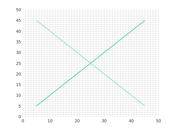
Compute CI and construct fracture grid
For each matrix block containing a fracture, we compute a fracture-matrix conductivity index (CI) in accordance with the hierarchical fracture model (a.k.a. embedded discrete fracture model). Following that, we compute a fracture grid where the fracture cell size is defined to be 0.5 m. Next, the fracture grid is plotted on top of the matrix grid.
dispif(mrstVerbose, 'Computing CI and constructing fracture grid...\n\n');
G = CIcalculator2D(G,fracture);
min_size = 0.5; cell_size = 0.5; % minimum and average cell size.
[G,F,fracture] = gridFracture2D(G,fracture,'min_size',min_size,'cell_size',cell_size);
clf; plotFractureNodes2D(G,F,fracture); box on
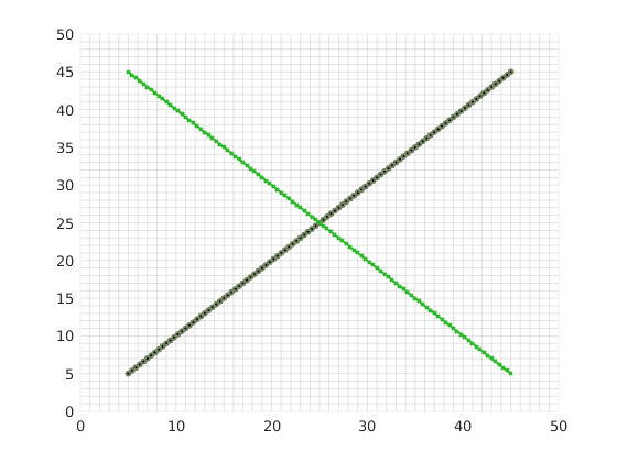
Make layered grid
Using makeLayers, we extrude the matrix grid and each fracture grid along the z-direction. The fracture grid is extruded and readjusted in accordance with ‘flayers’.
Gl = makeLayers(G,layers,flayers);
Set rock properties in fracture and matrix
For this example, we will generate the matrix porosity as a Gaussian field. To get a crude approximation to the permeability-porosity relationship, we assume that our medium is made up of uniform spherical grains of diameter dp = 10 m, for which the specic surface area is Av = 6 = dp. With these assumptions, using the Carman Kozeny relation, we can then calculate the isotropic matrix permeability (K). The rock properties are then plotted. Fracture permeability is set to 1000 Darcy with 50% porosity in each fracture grid cell. The rock properties are then plotted.
p = gaussianField(Gl.cartDims, [0.2 0.4], [9 5 5], 3.5);
K = p.^3.*(1e-5)^2./(0.81*72*(1-p).^2);

Gl.rock = makeRock(Gl, K(:), p(:));
K_frac = 10000; % Scaling factor = K_frac/K_mat D
poro_frac = 0.5;
Gl = makeRockFrac(Gl, K_frac, 'permtype','homogeneous','porosity',poro_frac);

clf; plotToolbar(Gl,Gl.rock);
colormap(jet); view (-135,30);
axis tight equal off
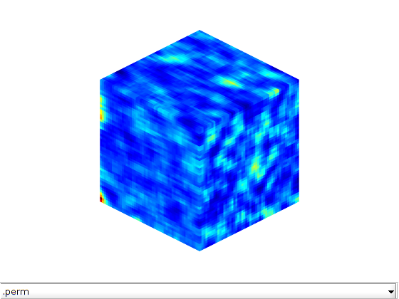
Define fluid properties
Define a single fluid of viscosity 1 cP and density 1000 kg/m3.
fluid = initSingleFluid('mu' , 1*centi*poise, ...
    'rho', 1000*kilogram/meter^3);
Global grid with NNC’s and corresponding transmissibility
In this section, we use the function makeNNCextruded to combine the layered fracture and matrix grid structures into a single grid structure. Additionally, we assign a ‘non-neighbouring connection (NNC)’ status to every fracture-matrix connection. For example, if fracture cell ‘i’ is located in the matrix cell ‘j’, then the connection i-j is defined as an NNC. To compute the flux between these elements, we compute a transmissibility for each NNC using the CI’s computed earlier. Vector T contains the transmissibility for each face in the combined grid and each NNC.
[Gl,T] = makeNNCextruded(G,Gl,F,fracture,flayers);
G = Gl; clear Gl
Add Wells
We will include two horizontal wells, a rate-controlled injector well through the bottom left corner of the grid and a producer, controlled by bottom-hole pressure, through the top right section of the grid. Wells are described using a Peaceman model, giving an extra set of equations that need to be assembled, see simpleWellExample.m for more details on the Peaceman well model.
[nx, ny, nz] = deal(G.cartDims(1), G.cartDims(2), G.cartDims(3));
cellinj = nx*ny*(nz-1)+1:nx:nx*ny*nz;
cellprod = nx:nx:nx*ny;

W = [];
W   = addWell(W, G.Matrix, G.Matrix.rock, cellinj, 'Type', 'rate',...
    'Val', 1000/day, 'Sign',1, 'Comp_i', 1, 'Name', 'Injector');
W   = addWell(W, G.Matrix, G.Matrix.rock, cellprod, ...
    'Type', 'bhp', 'Val', 50*barsa(), 'Sign', -1, 'Comp_i', 1, 'Name', 'Producer');
Initialize state variables
Once the transmissibilities are computed, we can generate the transmissiblity matrix ‘A’ using the ‘two-point flux approximation’ scheme and initialize the solution structure.
dispif(mrstVerbose, 'Computing coefficient matrix...\n\n');
state  = initResSol (G, 0);
state.wellSol = initWellSol(W, 0);
[A,q] = getSystemIncompTPFA(state, G, T, fluid, 'use_trans', true);
Solve fine-scale problem
The fine-scale pressure solution is computed using the boundary conditions provided and the transmissiblity matrix computed earlier.
dispif(mrstVerbose, '\nSolving fine-scale system...\n\n');
state_fs = incompTPFA(state, G, T, fluid,  ...
    'Wells', W, 'MatrixOutput', true, 'use_trans',true);
Setup multiscale grids
Next, we define a 10-by-10-by-10 matrix coarse grid such that each coarse block contains 5-by-5-by-5 fine cells. Each of the two fracture planes is partitioned into 3-by-3 coarse blocks. In total, the fracture grid has 18 degrees of freedom at coarse scale giving a coarsening ratio of ~333. Additionally, we also define the support regions for the fracture and matrix basis functions. Fracture support region is defined based on a topological distance based algorithm. The matrix and fracture coarse grids are plotted in the next section.
G.type{1,1} = 'layered';

% Partition matrix
coarseDims = [10 10 10];
pm = partitionMatrix(G, 'coarseDims', coarseDims, 'use_metis', false);
CGm = getRsbGridsMatrix(G, pm, 'fullyCoupled', false, 'Wells', W);

% Partition fracture
nw = fracture.network;
coarseDimsF = [3 3];
p  = partitionFracture(G, pm, nw, 'partition_frac'   , true   , ...
    'use_metisF'       , false  , ...
    'coarseDimsF'      , coarseDimsF );

p = processPartition(G,compressPartition(p));
pf = p(G.Matrix.cells.num+1:end)-max(p(1:G.Matrix.cells.num));

% Coarse Grids
CG = generateCoarseGrid(G, p);

% Add centroids / geometry information on coarse grid
CG = coarsenGeometry(CG);
Gf = assembleFracGrid(G);
CGf = generateCoarseGrid(Gf, pf);
CGf = coarsenGeometry(CGf);

% Support Regions
[CG,CGf] = storeFractureInteractionRegion(CG, CGf, CGm, ...
    'excludeBoundary' , false , ...
    'removeCenters'   , false , ...
    'fullyCoupled'    , false );
Compute basis functions
Using the transmissibility matrix ‘A’ we compute the basis functions for each fracture and matrix coarse block using the restriction smoothed basis method. Note that the matrix ‘A’ does not contain any source terms or boundary conditions. They are added to the coarse linear system when computing the multiscale pressure in the next section.
dispif(mrstVerbose, 'Computing basis functions...\n\n');
basis_sb = getMultiscaleBasis(CG, A, 'type', 'msrsb');
clf; plotToolbar(G,basis_sb.B,'filterzero',true); view(-135,30)
plotGrid(CG, 'FaceColor', 'none', 'linewidth', 1);
axis tight; colormap(jet); colorbar;
title('Basis Functions in the matrix');
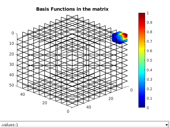
Compute multiscale solution
state_ms = incompMultiscale(state, CG, T, fluid, basis_sb, 'Wells', W, ...
    'use_trans',true);
Plot results
figure;
plotToolbar(G, state_fs.pressure)
colormap jet; colorbar
view(-135,30)
axis tight off
title('Fine scale')

figure;
plotToolbar(G, state_ms.pressure)
colormap jet; colorbar
view(-135,30)
axis tight off
title('F-MsRSB')

L1 = abs(state_ms.pressure-state_fs.pressure)./state_fs.pressure;
figure;
plotToolbar(G, L1)
colormap jet; colorbar
view(-135,30)
axis tight off
L1_eq = '$$| P_i^{fs}-P_i^{ms} | / P_i^{fs} $$';
title(L1_eq,'interpreter','latex');
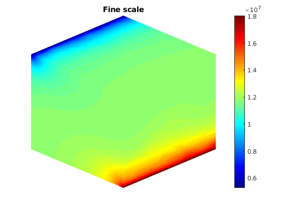
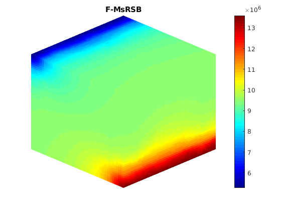
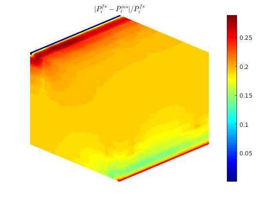
Solve using MS-ILU and MS-GMRES
As seen in the plots above, the multiscale method is able to capture the general trend of the solution, but can have large pointwise errors. To improve the approximation, we can compute iterative multiscale solutions using ILU and GMRES preconditioners.
fn = getSmootherFunction('type', 'ilu');

[~,report] = incompMultiscale(state, CG, T, fluid, basis_sb,...
    'Wells', W, 'use_trans', true, 'tolerance', 1e-8, 'iterations', 100,...
    'useGMRES', false, 'reconstruct', true, 'getSmoother', fn);

[~,report2] = incompMultiscale(state, CG, T, fluid, basis_sb,...
    'Wells', W, 'use_trans', true, 'tolerance', 1e-8, 'iterations', 100,...
    'useGMRES', true, 'reconstruct', true, 'getSmoother', fn);
Plot convergence
igure;
semilogy(report.resvec, ':+'); hold on;
semilogy(report2.resvec, 's-');
legend('Convergence of ILU(0)', 'Convergence of GMRES');
title('Iterative convergence');

% <html>
% <p><font size="-1