`mpfa`: Multi-point flux approximation solvers for pressure¶

Implementation of the multipoint flux-approximation (MPFA-O) method for incompressible (Poisson-type) pressure equations

Contents¶

Routines supporting the MPFA-O method for the pressure equation.

Files: computeMultiPointTrans - Compute multi-point transmissibilities. incompMPFA - Solve incompressible flow problem (fluxes/pressures) using MPFA-O method. matrixBlocksFromSparse - Extract block-diagonal matrix elements from sparse matrix

computeMultiPointTrans(g, rock, varargin)¶

Compute multi-point transmissibilities.

Synopsis:

T = computeMultiPointTrans(G, rock)

Parameters:

G – Grid data structure as described by grid_structure.
rock –
Rock data structure with valid field ‘perm’. The permeability is assumed to be in measured in units of metres squared (m^2). Use function ‘darcy’ to convert from (milli)darcies to m^2, e.g.,

perm = convertFrom(perm, milli*darcy)

if the permeability is provided in units of millidarcies.

The field rock.perm may have ONE column for a scalar permeability in each cell, TWO/THREE columns for a diagonal permeability in each cell (in 2/3 D) and THREE/SIX columns for a symmetric full tensor permeability. In the latter case, each cell gets the permeability tensor

K_i = [ k1 k2 ] in two space dimensions

[ k2 k3 ]

K_i = [ k1 k2 k3 ] in three space dimensions

[ k2 k4 k5 ] [ k3 k5 k6 ]

OPTIONAL PARAMETERS

verbose - Whether or not to emit informational messages throughout the: computational process. Default value depending on the settings of function ‘mrstVerbose’.

facetrans -

invertBlocks -

Method by which to invert a sequence of small matrices that arise in the discretisation. String. Must be one of

MATLAB – Use an function implemented purely in MATLAB

(the default).

MEX – Use two C-accelerated MEX functions to

extract and invert, respectively, the blocks along the diagonal of a sparse matrix. This method is often faster by a significant margin, but relies on being able to build the required MEX functions.

Returns:	T – half-transmissibilities for each local face of each grid cell in the grid. The number of half-transmissibilities equal the number of rows in G.cells.faces.

COMMENTS:: PLEASE NOTE: Face normals have length equal to face areas.

See also

incompMPFA, mrstVerbose.

incompMPFA(state, g, T, fluid, varargin)¶

Solve incompressible flow problem (fluxes/pressures) using MPFA-O method.

Synopsis:

state = incompMPFA(state, G, T, fluid)
state = incompMPFA(state, G, T, fluid, 'pn1', pv1, ...)

Description:

This function assembles and solves a (block) system of linear equations defining interface fluxes and cell pressures at the next time step in a sequential splitting scheme for the reservoir simulation problem defined by Darcy’s law and a given set of external influences (wells, sources, and boundary conditions).

This function uses a multi-point flux approximation (MPFA) method with minimal memory consumption within the constraints of operating on a fully unstructured polyhedral grid structure.

Keyword Arguments:
Parameters:	state – Reservoir and well solution structure either properly initialized from functions ‘initResSol’ and ‘initWellSol’ respectively, or the results from a previous call to function ‘incompMPFA’ and, possibly, a transport solver such as function ‘implicitTransport’. T (G,) – Grid and half-transmissibilities as computed by the function ‘computeMultiPointTrans’. fluid – Fluid object as defined by function ‘initSimpleFluid’.
	W – Well structure as defined by functions ‘addWell’ and ‘assembleWellSystem’. May be empty (i.e., W = struct([])) which is interpreted as a model without any wells. bc – Boundary condition structure as defined by function ‘addBC’. This structure accounts for all external boundary conditions to the reservoir flow. May be empty (i.e., bc = struct([])) which is interpreted as all external no-flow (homogeneous Neumann) conditions. src – Explicit source contributions as defined by function ‘addSource’. May be empty (i.e., src = struct([])) which is interpreted as a reservoir model without explicit sources. LinSolve – Handle to linear system solver software to which the fully assembled system of linear equations will be passed. Assumed to support the syntax x = LinSolve(A, b) in order to solve a system Ax=b of linear equations. Default value: LinSolve = @mldivide (backslash). MatrixOutput – Whether or not to return the final system matrix ‘A’ to the caller of function ‘incompMPFA’. Logical. Default value: MatrixOutput = FALSE. Verbose – Whether or not to time portions of and emit informational messages throughout the computational process. Logical. Default value dependent on global verbose setting in function ‘mrstVerbose’.
Returns:	xr – Reservoir solution structure with new values for the fields: - pressure – Pressure values for all cells in the discretised reservoir model, ‘G’. boundaryPressure – Pressure values for all boundary interfaces in the discretised reservoir model, ‘G’. flux – Flux across global interfaces corresponding to the rows of ‘G.faces.neighbors’. A – System matrix. Only returned if specifically requested by setting option ‘MatrixOutput’. xw – Well solution structure array, one element for each well in the model, with new values for the fields: flux – Perforation fluxes through all perforations for corresponding well. The fluxes are interpreted as injection fluxes, meaning positive values correspond to injection into reservoir while negative values mean production/extraction out of reservoir. pressure – Well pressure.

Note

If there are no external influences, i.e., if all of the structures ‘W’, ‘bc’, and ‘src’ are empty and there are no effects of gravity, then the input values ‘xr’ and ‘xw’ are returned unchanged and a warning is printed in the command window. This warning is printed with message ID

‘incompMPFA:DrivingForce:Missing’

Example:

G   = computeGeometry(cartGrid([3,3,5]));
f   = initSingleFluid('mu' ,    1*centi*poise     , ...
                      'rho', 1014*kilogram/meter^3);
rock.perm = rand(G.cells.num, 1)*darcy()/100;
bc  = pside([], G, 'LEFT', 2);
src = addSource([], 1, 1);
W   = verticalWell([], G, rock, 1, G.cartDims(2), ...
                   (1:G.cartDims(3)), 'Type', 'rate', 'Val', 1/day(), ...
                   'InnerProduct', 'ip_tpf');
W   = verticalWell(W, G, rock, G.cartDims(1),   G.cartDims(2), ...
                   (1:G.cartDims(3)), 'Type', 'bhp', ...
                   'Val',  1*barsa(), 'InnerProduct', 'ip_tpf');
T   = computeMultiPointTrans(G, rock);

state = initState(G, W, 100*barsa);
state = incompMPFA(state, G, T, f, 'bc', bc, 'src', src, ...
                   'W', W, 'MatrixOutput',true);

plotCellData(G, xr.pressure);

Examples¶

Example 1: Cartesian Grid with Anistropic Permeability¶

Generated from mpfaExample1.m

The multipoint flux-approximation (MPFA-O) method is developed to be consistent on grids that are not K-orthogonal. In this example, we introduce how to use the method by applying it to a problem with anisotropic permeability. For comparison, we also compute solutions with two other methods: (i) the two-point flux-approximation (TFPA) method, which is not consistent and only convergent on K-orthogonal grids; and the mimetic finite-difference (MFD) method, which is consistent and applicable to general polyhedral grids. For the MFD method, we will use an inner product that simplifies to a two-point method on K-orthogonal grids. To compare the methods, we consider the single-phase pressure equation

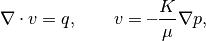
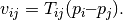
$\nabla\cdot v = q, \qquad v=\textbf{--}\frac{K}{\mu}\nabla p,$

for a two-dimensional Cartesian grid with anisotropic, homogeneous permeability which will violate the K-orthogonality condition. To drive the flow, we impose a single well and zero Dirichlet boundary conditions. The main idea of the TPFA method is to approximate the flux v over a face f by the difference of the cell centered pressures in the neighboring cells (sharing the face f) weigthed by a face transmissibility T:

$v_{ij} = T_{ij}(p_i \textbf{--} p_j).$

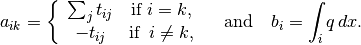
The pressure in each cell is approximated by solving a linear system Ap = b. When ignoring wells, sources, and bc, A and b are given by

$a_{ik} = \left\{\begin{array}{cc} \sum_j t_{ij} & \textrm{if } i=k, \\ -t_{ij} & \textrm{if }\, i\neq k, \end{array} \right. \quad \textrm{and} \quad b_i = \int_{i} q \, dx.$

Once the pressure is known, the flux is calculated using the expression given above. In the same manner, the MPFA method approximates the flux v over a face f as a linear combination of the cell pressure and cell pressures in neighbor cells sharing at least one vertex with the face f. The mimetic method approximates the face flux as a linear combination of cell pressures and face pressures. Only in special cases is it possible to make a local stencil for the face flux in terms of cell pressures, while the stencil for the flux in terms of face pressures is always local. In this example we show non-monotone solutions to the pressure equation that arise from both the MPFA-method and the Mimetic method.

verbose = false;
MODS = mrstModule;
mrstModule add mimetic mpfa incomp

Define and process geometry¶

Construct a Cartesian grid of size 10-by-10-by-4 cells, where each cell has dimension 1-by-1-by-1. Because our flow solvers are applicable for general unstructured grids, the Cartesian grid is here represented using an unstructured formate in which cells, faces, nodes, etc. are given explicitly.

nx = 11; ny = 11;
G = cartGrid([nx, ny]);
G = computeGeometry(G);

Set rock and fluid data¶

The only parameters in the single-phase pressure equation are the permeability

, which here is homogeneous, isotropic and equal 100 mD. The fluid has density 1000 kg/m^3 and viscosity 1 cP. We make a non diagonal rock tensor

theta=30*pi/180;
U=[cos(theta),sin(theta);-sin(theta),cos(theta)];
rocktensor = U'*diag([0.1,10])*U;
rocktensor =[rocktensor(1,1),rocktensor(1,2),rocktensor(2,2)];
rock = makeRock(G, rocktensor .* 1e-3*darcy, 1);
fluid     = initSingleFluid('mu' ,    1*centi*poise     , ...
                            'rho', 1014*kilogram/meter^3);

gravity off

Introduce wells¶

We will include two wells, one rate-controlled vertical well and one horizontal well controlled by bottom-hole pressure. Wells are described using a Peacemann model, giving an extra set of equations that need to be assembled. We need to specify (‘InnerProduct’, ‘ip_tpf’) to get the correct well model for TPFA. The first well is vertical well (vertical is default):

cellsWell1 =  sub2ind(G.cartDims,floor(nx/2)+1,floor(ny/2)+1);
radius     = .1;
% well with wellindex calculated for TPFA
bhp=1;
W = addWell([], G, rock, cellsWell1, 'Comp_i', 1, ...
            'Type', 'bhp', 'Val', bhp*barsa(),    ...
            'Radius', radius, 'InnerProduct', 'ip_tpf');
% well with wellindex calculated for MIMETIC
W_mim = addWell([], G, rock, cellsWell1, 'Comp_i', 1, ...
            'Type', 'bhp', 'Val', bhp*barsa(),        ...
            'Radius', radius, 'InnerProduct', 'ip_simple');

Impose Dirichlet boundary conditions¶

Our flow solvers automatically assume no-flow conditions on all outer (and inner) boundaries; other type of boundary conditions need to be specified explicitly. Here, we impose Neumann conditions (flux of 1 m^3/day) on the global left-hand side. The fluxes must be given in units of m^3/s, and thus we need to divide by the number of seconds in a day (day()). Similarly, we set Dirichlet boundary conditions p = 0 on the global right-hand side of the grid, respectively. For a single-phase flow, we need not specify the saturation at inflow boundaries. Similarly, fluid composition over outflow faces (here, right) is ignored by pside.

bc = pside([], G, 'LEFT',  0);
bc = pside(bc, G, 'RIGHT', 0);
bc = pside(bc, G, 'BACK', 0);
bc = pside(bc, G, 'FRONT', 0);

APPROACH 1: Direct/Classic TPFA¶

Initialize solution structure with reservoir pressure equal 0. Compute one-sided transmissibilities for each face of the grid from input grid and rock properties. The harmonic averages of ones-sided transmissibilities are computed in the solver incompTPFA.

T = computeTrans(G, rock);

Initialize well solution structure (with correct bhp). No need to assemble well system (wells are added to the linear system inside the incompTPFA-solver).

resSol1 = initState(G, W, 0);

% Solve linear system construced from T and W to obtain solution for flow
% and pressure in the reservoir and the wells. Notice that the TPFA solver
% is different from the one used for mimetic systems.
resSol1 = incompTPFA(resSol1, G, T, fluid, 'wells', W, 'bc',bc);

APPROACH 2: Mimetic with TPFA-inner product¶

Initialize solution structure with reservoir pressure equal 0. Compute the mimetic inner product from input grid and rock properties.

IP = computeMimeticIP(G, rock, 'InnerProduct', 'ip_simple');
resSol2 = initState(G, W, 0);

Solve mimetic linear hybrid system¶

resSol2 = incompMimetic(resSol2, G, IP, fluid, 'wells', W_mim, 'bc', bc);

APPROACH 3: MPFA method¶

Compute the transmisibility matrix for mpfa

T_mpfa = computeMultiPointTrans(G, rock,'eta',1/3);
resSol3 = initState(G, W, 0);

Solve MPFA pressure¶

resSol3 = incompMPFA(resSol3, G, T_mpfa, fluid, 'wells', W,'bc',bc);

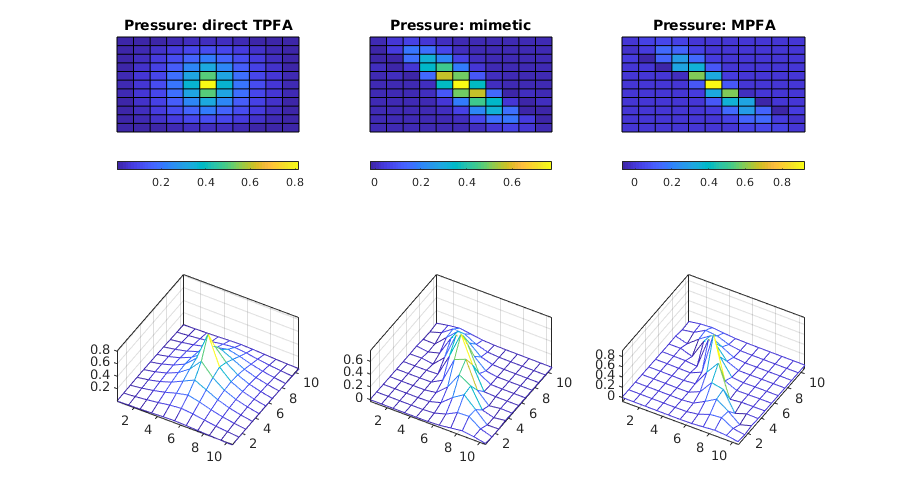
Plot solutions¶

Plot the pressure and producer inflow profile make Caresian grid

X=reshape(G.cells.centroids(:,1),G.cartDims);
Y=reshape(G.cells.centroids(:,2),G.cartDims);
clf
p = get(gcf,'Position'); set(gcf,'Position', [p(1:2) 900 500]);
subplot(2,3,1)
   plotCellData(G, resSol1.pressure(1:G.cells.num) ./ barsa());
   title('Pressure: direct TPFA'); view(2), axis tight off
   colorbar('Location','SouthOutside');
subplot(2,3,4)
   mesh(X,Y,reshape(resSol1.pressure(1:G.cells.num) ./ barsa(),G.cartDims));
   axis tight, box on, view(30,60);

subplot(2,3,2)
   plotCellData(G, resSol2.pressure(1:G.cells.num) ./ barsa());
   title('Pressure: mimetic'), view(2), axis tight off
   colorbar('Location','SouthOutside');
subplot(2,3,5)
   mesh(X,Y,reshape(resSol2.pressure(1:G.cells.num) ./ barsa(),G.cartDims));
   axis tight, box on, view(30,60);

subplot(2,3,3)
   plotCellData(G, resSol3.pressure(1:G.cells.num) ./ barsa());
   title('Pressure: MPFA'); view(2), axis tight off
   colorbar('Location','SouthOutside');
subplot(2,3,6)
   mesh(X,Y,reshape(resSol3.pressure(1:G.cells.num) ./ barsa(),G.cartDims));
   axis tight, box on, view(30,60);

% display the flux in the well for tpfa, mimetic and mpfa
disp('');
disp('Flux in the well for the three different methods:');
disp(['     TPFA   : ',num2str(resSol1.wellSol(1).flux .* day())]);
disp(['     Mimetic: ',num2str(resSol2.wellSol(1).flux .* day())]);
disp(['     MPFA-O : ',num2str(resSol3.wellSol(1).flux .* day())]);

Flux in the well for the three different methods:
     TPFA   : 0.060183
     Mimetic: 0.036858
     MPFA-O : 0.025232

mrstModule clear
mrstModule('add', MODS{:})

<html>
% <p><font size="-1

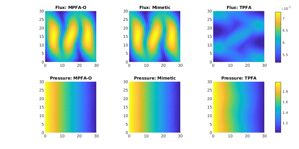
Example 2: Grid-orientation effect¶

Generated from mpfaExample2.m

The multipoint flux-approximation (MPFA-O) scheme is developed to be consistent on grids that are not necessarily K-orthogonal. This example demonstrates the basic use of the MPFA-O pressure solver by applying it to a single-phase flow problem posed on a square [0,30]x[0,30] m^2 with homogeneous and isotropic permeability. To discretize the problem, we introduce a skewed, curvilinear grid in which the majority of the grid cells are not K-orthogonal. The classical TPFA scheme can therefore be expected to give significant grid-orientation effects. To investigate this, we consider a single-phase flow problem with a prescribed pressure drop from the left to the right boundary, which gives an analytical solution p(x,y)=2-x/30. We compare the MPFA-O solution with solutions computed by the TPFA method and a mimetic method.

mrstModule add incomp mimetic mpfa

Set up simulation model¶

gravity off
G = cartGrid([30, 30]);
G.nodes.coords = twister(G.nodes.coords);
G = computeGeometry(G);

rock.perm = 0.1*darcy*ones(G.cells.num, 1);

bc  = pside([], G, 'left',  2);
bc  = pside(bc, G, 'right', 1);

fluid = initSingleFluid('mu' ,    1*centi*poise     , ...
                        'rho', 1014*kilogram/meter^3);

MPFA-O method¶

fprintf('MPFA-O method\t...
')
tic
T1  = computeMultiPointTrans(G, rock);
xr1 = incompMPFA(initResSol(G, 0, 0), G, T1, fluid, ...
                 'bc', bc,'MatrixOutput',true);
toc

MPFA-O method ... Elapsed time is 0.227233 seconds.

Mimetic method¶

fprintf('Mimetic method\t...
')
tic
S = computeMimeticIP(G, rock);
xr2 = incompMimetic(initResSol(G, 0, 0), G, S, fluid, 'bc', bc);
toc

Mimetic method        ... Elapsed time is 0.111970 seconds.

TPFA method¶

fprintf('TPFA Method\t...
')
tic
T2  = computeTrans(G, rock);
xr3 = incompTPFA(initResSol(G, 0, 0), G, T2, fluid, ...
                 'bc', bc,'MatrixOutput',true);
toc

TPFA Method   ... Elapsed time is 0.015765 seconds.

Plot solutions¶

hf2cn      = gridCellNo(G);
flux_int   = @(x) accumarray(hf2cn, abs(x.flux(G.cells.faces(:,1))));
plot_var   = @(v) plotCellData(G, v, 'EdgeColor','none');
plot_press = @(x) plot_var(x.pressure(1:G.cells.num));
plot_flux  = @(x) plot_var(convertTo(flux_int(x), meter^3/day));

clf, set(gcf,'Position',[300 250 1000 500]);

subplot(2,3,1),
plot_flux(xr1); cax=caxis();  axis equal tight, title('Flux: MPFA-O')

subplot(2,3,2),
plot_flux(xr2); caxis(cax); axis equal tight, title('Flux: Mimetic')

subplot(2,3,3),
plot_flux(xr3); caxis(cax);  axis equal tight, title('Flux: TPFA')
colorbar('Position',[.92 .58 .02 .34])

subplot(2,3,4),
plot_press(xr1); cax=caxis();  axis equal tight, title('Pressure: MPFA-O')

subplot(2,3,5),
plot_press(xr2); caxis(cax); axis equal tight, title('Pressure: Mimetic')

subplot(2,3,6),
plot_press(xr3); caxis(cax);  axis equal tight, title('Pressure: TPFA')
colorbar('Position',[.92 .11 .02 .34])

Compute discrepancies in flux and errors in pressure¶

= struct();
p.pressure = 2 - G.cells.centroids(:,1)/G.cartDims(1);
err_press  = @(x1, x2) ...
    norm(x1.pressure - x2.pressure, inf) / norm(x1.pressure, inf);
err_flux   = @(x1, x2) norm(flux_int(x1) - flux_int(x2), inf);

fprintf(['\nMaximum difference in face fluxes:\n', ...
         '\to MPFA-O /TPFA   : %.15e\n',   ...
         '\to MPFA-O /Mimetic: %.15e\n',   ...
         '\to Mimetic/TPFA   : %.15e\n\n', ...
         ], ...
        err_flux(xr1, xr3), err_flux(xr1, xr2), err_flux(xr2, xr3));

fprintf(['Relative error in cell pressures:\n', ...
         '\to MPFA-O         : %.15e\n',  ...
         '\to Mimetic        : %.15e\n',  ...
         '\to TPFA           : %.15e\n',  ...
         ], ...
         err_press(xr1, p), err_press(xr2, p), err_press(xr3, p));

Maximum difference in face fluxes:
      o MPFA-O /TPFA   : 2.299989914878246e-12
      o MPFA-O /Mimetic: 1.597815675419813e-24
      o Mimetic/TPFA   : 2.299989914878142e-12

Relative error in cell pressures:
      o MPFA-O         : 5.593419636395030e-15
...

mpfa: Multi-point flux approximation solvers for pressure¶

Examples¶

Example 1: Cartesian Grid with Anistropic Permeability¶

Define and process geometry¶

Set rock and fluid data¶

Introduce wells¶

Impose Dirichlet boundary conditions¶

APPROACH 1: Direct/Classic TPFA¶

APPROACH 2: Mimetic with TPFA-inner product¶

Solve mimetic linear hybrid system¶

APPROACH 3: MPFA method¶

Solve MPFA pressure¶

Plot solutions¶

Example 2: Grid-orientation effect¶

Set up simulation model¶

MPFA-O method¶

Mimetic method¶

TPFA method¶

Plot solutions¶

Compute discrepancies in flux and errors in pressure¶

`mpfa`: Multi-point flux approximation solvers for pressure¶