`coarsegrid`: Generation of coarse grids¶

Utilities¶

Contents¶

COARSEGRID

Files: cellPartitionToFacePartition - Construct partition of all grid faces from cell partition. compressPartition - Renumber coarse block partitioning to remove any empty coarse blocks. generateCoarseGrid - Form coarse grid from partition of fine-scale grid. partitionCartGrid - Partition a Cartesian grid. partitionLayers - Partition grid uniformly in logical (I,J) direction, non-uniformly in K. partitionMETIS - Partition grid according to connection strengths partitionUI - Partition grid uniformly in logical space. partitionTensor - Partition Logically Cartesian Grid Into Tensor Product Blocks processFacePartition - Ensure that all coarse faces are connected collections of fine faces. processPartition - Split disconnected coarse blocks into new blocks. refineNearWell - Partition a set of points based on proximity to a well point sortSubEdges - Sorts subfaces in a 2D coarse grid. subFaces - Extract fine-grid faces constituting individual coarse grid faces.

cellPartitionToFacePartition(g, p, varargin)¶

Construct partition of all grid faces from cell partition.

Synopsis:

pf = cellPartitionToFacePartition(g, p)
pf = cellPartitionToFacePartition(g, p, 'pn1', pv1, ...)

Description:

Define unique partition ID for each pair of cell partition IDs occurring in a partition vector, and construct a partitioning of all faces in a grid.

Parameters:

g – Grid structure as described by grid_structure.
p – Cell partition
'pn'/pv –
List of ‘key’/value pairs for supplying optional parameters. The supported options are

AllBoundaryFaces -

Flag indicating whether or not every fine-scale boundary face should be assigned a separate, unique partition ID number to force individual inclusion in the coarse grid.
Logical. Default value: AllBoundaryFaces=false (do not assign separate partition IDs to each fine-grid boundary face).

Returns:

pf – Face partition. One non-negative integer per face in ‘g’. Fine-scale faces that are not on the boundary between coarse blocks are assigned a partition ID number of zero.

See also

processFacePartition

compressPartition(p)¶

Renumber coarse block partitioning to remove any empty coarse blocks.

Synopsis:

p = compressPartition(p)

Parameters:	p – Original partition vector, may contain empty coarse blocks.
Returns:	p – Updated partition vector. Renumbered so as to remove empty coarse blocks.

Note

If the original partition does not contain any empty coarse blocks, applying this function is an expensive way of doing nothing.

Example:

p = partitionCartGrid([4, 4, 1], [2, 2, 2]);
[p, compressPartition(p)]

generateCoarseGrid(G, p, varargin)¶

Form coarse grid from partition of fine-scale grid.

Synopsis:

CG = generateCoarseGrid(G, pv)
CG = generateCoarseGrid(G, pv, pf)

Parameters:

G – grid_structure data structure describing fine-scale discretisation of reservoir geometry.
pv – Partition vector of size [G.cells.num, 1] describing the coarse grid. We assume that all coarse blocks are connected. The partition vector is often created by function partitionCartGrid or function partitionUI.
pf – Partition vector on faces of ‘G’. This indicator enables construction of coarse grids with multiple connections between coarse block pairs. OPTIONAL. Default value (unset) corresponds to generating coarse faces defined by unique block pairs only.

Returns:

CG – Coarse grid structure. A master structure having the following
fields –
- cells –
  
  A structure specifying properties for each individual block in the grid. See CELLS below for details.
- faces –
  
  A structure specifying properties for each individual block connections in the grid. See FACES below for details.
- partition –
  
  A copy of the partition vector ‘pv’
- parent –
  
  A copy of the grid structure for the parent grid
- type –
  
  A cell array of strings describing the history of grid constructor and modifier functions through which a particular grid structure has been defined.
- griddim –
  
  The dimension of the grid which in most cases will equal ‘size(G.nodes.coords,2)’.
CELLS – Cell structure G.cells: - num –

Number of cells in global grid.
- facePos –
  
  Indirection map of size [num+1,1] into the ‘cells.faces’ array. Specifically, the connection information of block ‘i’ is found in the submatrix
  
  CG.cells.faces(facePos(i) : facePos(i+1)-1, :)
  
  The number of connections of each block may be computed using the statement DIFF(facePos).
- faces –
  
  A (CG.cells.facePos(end)-1)-by-2 array of global connections associated with a given block. Specifically, if ‘cells.faces(i,1)==j’, then global connection ‘cells.faces(i,2)’ is associated with global block ‘j’.
  
  To conserve memory, only the second column is actually stored in the grid structure. The first column may be reconstructed using the statement
  
  rldecode(1 : CG.cells.num, diff(CG.cells.facePos), 2) .’
  
  Optionally, one may append a third column to this array that contains a tag that has been inherited from the parent grid.
FACES – Face structure G.faces: - num –

Number of global connections in grid.
- connPos, fconn –
  
  Packed data-array representation of coarse->fine connection mapping. Specifically, the elements
  
  fconn(connPos(i) : connPos(i + 1) - 1)
  
  are the connections in the parent grid (i.e., rows of the neighborship definition ‘G.faces.neighbors’) that constitute coarse-grid connection ‘i’.
- neighbors –
  
  A CG.faces.num-by-2 array of neighbouring information. Global connection ‘i’ is shared by global blocks neighbors(i,1) and neighbors(i,2). One of ‘neighbors(i,1)’ or ‘neighbors(i,2)’, but not both, may be zero, meaning that connection ‘i’ is between a single block and the exterior of the grid.
The coarse grid consists entirely of topological information
stored in the same topological fields as in the fine – scale grid
described in ‘grid_structure’. Specifically, the fields – CG.cells.num, CG.cells.facePos, CG.cells.faces CG.faces.num, and CG.faces.neighbors
have the same interpretation in the coarse grid as in the
fine – scale grid.

partitionCartGrid(cartDims, partDims)¶

Partition a Cartesian grid.

Synopsis:

partition = partitionCartGrid(cartDims, partDims)

Parameters:	cartDims – [nx ny nz] vextor of fine-grid cell dimensions. partDims – [cnx cny cnz] vector of coarse-grid block dimensions.
Returns:	partition – Vector of size [nxnynz 1] with entries equal to coarse block index.

See also

processPartition.

partitionLayers(G, coarseDim, L)¶

Partition grid uniformly in logical (I,J) direction, non-uniformly in K.

Synopsis:

blockIx = partitionLayers(G, coarseDim, L)

Description:

Partitions a corner point grid in grid_structure format (relatively) non-uniformly in k-direction and uniformly in ij-directions in index (logical) space. In the ij-directions, each coarse block is comprised of roughly the same number of cells from the fine grid.

Parameters:	G – grid_structure structure having either a valid field ‘G.cells.ijkMap’ or both valid fields ‘G.cartDims’ and ‘G.cells.indexMap’. coarseDim – Number of coarse blocks in each ij direction. Assumed to be a LENGTH 2 vector of integers. L – A run-length-encoded vector of the desired layers.
Returns:	blockIx – A G.cells.num-by-1 vector mapping cells to coarse blocks.

Example:

See simpleCornerPointExampleMS

See also

processPartition, partitionUI.

partitionMETIS(G, T, n, varargin)¶

Partition grid according to connection strengths

Synopsis:

p = partitionMETIS(G, T, n)
p = partitionMETIS(G, T, n, 'pn1', pv1, ...)

Keyword Arguments:
Parameters:	G – Grid structure. T – One-sided transmissibilities as defined by function ‘computeTrans’. Possibly affected by mobility. n – Number of blocks into which to partition the grid ‘G’.
	ufactor – Percentage overweight allowed in coarse blocks. Examples: 1.01: Largest difference in cells per coarse block is equal to or less than 1%. 1.50: Largest difference in cells per coarse block is equal to or less than 50%. (DEFAULT) no2hop – Do not use multiple hops when coarsening. Passed onto METIS. seed – METIS seeding parameter to create consistent results for given platform. Default: 0. ncuts – Passed onto METIS. useLog – Log_10 transform transmissibilities before creating connection matrix. This can be useful when transmissibilities vary by several orders of magnitude locally.
Returns:	p – Partition vector. Contains no empty or multiply connected blocks. A – Matrix used for partitioning.

partitionTensor(G, di, dj, dk)¶

Partition Logically Cartesian Grid Into Tensor Product Blocks

Synopsis:

% In two space dimensions
p = partitionTensor(G, di, dj)

% In three space dimensions
p = partitionTensor(G, di, dj, dk)

Parameters:

G – MRST grid as described in grid_structure. Assumed to carry an underlying logically Cartesian structure (i.e., each cell can be identified by its (I,J) pair or (I,J,K) triplet in two and three space dimensions, respectively.
di,dj,dk –
Tensor product block sizes. Vectors of positive integers. Specifically, the block at position (x,y,z) consists of

di(x)-by-dj(y)-by-dk(z)

cells from the underlying fine-scale grid (i.e., G)–at least if all cells are active. These inputs play the same roles, and are subject to the same restrictions like

ALL([SUM(di), SUM(dj), SUM(dk)] == G.cartDims)

as the ‘dimDist’ inputs of function MAT2CELL.

Returns:

p – Partition vector. Contains no empty or multiply connected blocks.

See also

partitionUI, partitionLayers, mat2cell.

partitionUI(G, coarseDim)¶

Partition grid uniformly in logical space.

Synopsis:

blockIx = partitionUI(G, coarseDim)

Description:

Partitions a corner point grid in grid_structure format (relatively) uniformly in index (logical) space. Each coarse block is comprised of roughly the same number of cells from the fine grid.

Parameters:	G – grid_structure structure having valid ‘G.cartDims’ and ‘G.cells.indexMap’ fields. coarseDim – Number of coarse blocks in each physical direction. Assumed to be a LENGTH 2 or 3 vector of integers.
Returns:	blockIx – A G.cells.num-by-1 vector mapping cells to coarse blocks.

See also

processPartition, partitionLayers.

processFacePartition(g, p, pf)¶

Ensure that all coarse faces are connected collections of fine faces.

Synopsis:

pf = processFacepartition(g, p, pf)

Parameters:	g – Grid structure as described by grid_structure. p – Partition vector of size [G.cells.num, 1] describing the coarse grid. We assume that all coarse blocks are connected. The partition vector is often created by function partitionCartGrid or function partitionUI. pf – Partition vector on faces of ‘G’.
Returns:	pf – Processed partition face vector.

COMMENTS:: Currently only implemented for 2D grids.

processPartition(G, partition, facelist)¶

Split disconnected coarse blocks into new blocks.

Synopsis:

q = processPartition(G, p)
q = processPartition(G, p, facelist)

Parameters:

G – Grid structure as described by grid_structure.
p – Vector of size G.cells.num-by-1 of initial cell-to-block mappings. Assumed to be a vector of positive integers. The coarse block numbers are preserved for all blocks that are internally connected. Consequently, if all coarse blocks are connected then ALL(q == p).
facelist – List of faces across which the connections between cells should be removed before the processing

Returns:

q – Updated partition with only connected coarse blocks.

refineNearWell(pts, wellpt, varargin)¶

Partition a set of points based on proximity to a well point

Synopsis:

p = refineNearWell(points, wellpoint)

Parameters:

pts – Set of points that are to be partitioned (for example G.cells.centroids)
wellpt – A single point to be used for partitioning (for example the well heel. Routine currently only partitions in xy-plane.

Keyword Arguments:

maxRadius – The distance in meters for which a partition will be applied. (Defaults to inf, i.e. all points). If maxRadius is a two-vector, the partition is applied inside a rectangle rather than inside a circle.
angleBins – The number of sectors the region will be divided into along the angle around the point.
radiusBins – Number of distinct regions produced as the radius increases.
logBins – If true (default) then the radius bins will have width that drops off as a log(r). Otherwise, will distribute in a linear fashion.

Returns:

p – Partition vector. One entry for each point. Will contain: zero for any points that are out of bounds for the maxRadius parameter.

binAngle - The partition used for the sector partitioning.

binRadius - The partition used for the radius partitioning.

dist - Distance per point used for cutoff by maxRadius.

See also

grid_structure, generateCoarseGrid.

Contents¶: Files callMetisMatrix - Partition connectivity graph whilst accounting for connection strengths coarseDataToFine - Convert coarse grid dataset into fine grid representation coarsenBC - Construct coarse-grid boundary conditions from fine-grid boundary cond. coarsenFlux - Compute net flux on coarse faces coarsenGeometry - Add geometry (centroids, face normals, areas, …) to a coarse grid fineToCoarseSign - Compute sign change between fine faces and coarse faces. invertPartition - Invert partition (cell->block mapping) to create block->cell mapping. isSamePartition - Check if two partition vectors represent the same grid partition

callMetisMatrix(A, n, varargin)¶

Partition connectivity graph whilst accounting for connection strengths

Synopsis:

p = callMetisMatrix(A, n)

Parameters:

A – Symmetric connectivity graph represented as a sparse matrix. The magnitude (absolute value) of the off-diagonal non-zero entries is used to measure the strengths of the individual connections.
n – Number of blocks into which the vertices of the connectivity graph ‘A’ should be partitioned. Must be an integer value exceeding one.
x – Any additional arguments will be interpreted as options, and will require metis5 to be installed. The function will then call gpmetis.

Returns:

p – A SIZE(A,1)-by-1 partition vector with semantics similar to those implied by other partitioning functions such as ‘partitionUI’.

Note

This function is a simple wrapper around the ‘kmetis’ or ‘gpmetis’ utilities from the METIS package (http://glaros.dtc.umn.edu/gkhome/metis/metis/overview). The ‘kmetis’/ ‘gpmetis’ utility is invoked through ‘system’ on a temporary file whose name is constructed by the ‘tempname’ function.

If the METIS function is not avilable in the search path used by the ‘system’ function, then function ‘callMetisMatrix’ will fail and an appropriate diagnostic message will be issued to the command window. To inform the system about where to find METIS, we use a global variable ‘METISPATH’ that can be set in your ‘startup_user’ function. If you, for instance, use Linux and have installed METIS in /usr/local/bin, you add the following line to your ‘startup_user’ file:

global METISPATH; METISPATH = fullfile(‘/usr’,’local’,’bin’);

Example:

% Partition a 10-by-10-by-3 Cartesian grid into 10 blocks according to
% the transmissibility field derived from isotropic permeabilities.
%
G = computeGeometry(cartGrid([10, 10, 3]));
K = convertFrom(10 * logNormLayers(G.cartDims), milli*darcy);
rock = struct('perm', K);

T = computeTrans(G, rock);
t = 1 ./ accumarray(G.cells.faces(:,1), 1 ./ T, [G.faces.num, 1]);

i = ~ any(G.faces.neighbors == 0, 2);
N = double(G.faces.neighbors(i, :));
A = sparse(N, fliplr(N), [ t(i), t(i) ]);

p = callMetisMatrix(A, 10);

See also

callMetis, partitionUI, processPartition, system, tempname.

coarseDataToFine(CG, data)¶: Convert coarse grid dataset into fine grid representation

coarsenBC(cg, bc)¶

Construct coarse-grid boundary conditions from fine-grid boundary cond.

Synopsis:

bc = coarsenBC(cg, bc)

Description:

All ‘pressure’ boundary conditions are mapped from fine-grid to the coarse-grid faces by sampling the value at cg.faces.centerFace *). All flux boundaries are accumulated

Parameters:	cg – Coarse-grid including parent grid. bc – MRST boundary conditions struct as returned by addBC.
Returns:	bc – MRST boundary conditions for coarse-grid cg. For ‘pressure’ conditions, the value is sampled in cg.faces.centerFace. For ‘flux’ conditions, the nex flux accoss the coarse face is computed. Mixed conditions are not supported.

coarsenFlux(cg, flux)¶

Compute net flux on coarse faces

Synopsis:

cflux = coarsenFlux(cg, flux)

Parameters:	cg – Coarse grid including parent grid. flux – Fine grid fluxes.
Returns:	cflux – Accumulated net flux on coarse faces

See also

coarsenGeometry, coarseConnections

coarsenGeometry(cg)¶

Add geometry (centroids, face normals, areas, …) to a coarse grid

Synopsis:

cg = coarsenGeometry(cg)

Parameters:	cg – Coarse grid including parent (fine) grid. (New definition).
Returns:	cg – Coarse grid with accumulated areas or volumes, area- or volume-weighted centroids and accumulated area-weighted normals accounting for sign convention in coarse and fine grid.

Note

The coarse geometry is derived from the geometry on the underlying fine grid. For this reason, the underlying fine grid should be the output from a call to computeGeometry(G).

See also

generateCoarseGrid, computeGeometry

fineToCoarseSign(cg)¶

Compute sign change between fine faces and coarse faces.

Synopsis:

sgn = fineToCoarseSign(cg)

Parameters:	cg – Coarse grid including parent (fine) grid. (New definition).
Returns:	sgn – fine-to-coarse sign for fine faces in cg.faces.fconn.

invertPartition(p)¶

Invert partition (cell->block mapping) to create block->cell mapping.

Synopsis:

[b2c_pos, b2c, locno] = invertPartition(p)

Parameters:

p – Partition vector.

Returns:

b2c_pos – Indirection map of size [MAX(p) + 1, 1] into the ‘b2c’ map array. Specifically, the cells of block ‘b’ are stored in

b2c(b2c_pos(b) : b2c_pos(b + 1) - 1)
b2c – Inverse cell map. The entries in b2c_pos(b) : b2c_pos(b+1)-1 correspond to the result of FIND(p == b).
locno –

A SIZE(p) array of local cell numbers. Specifically,

locno(c) == i

means that cell ‘c’ is the ‘i’th cell of block p(c).

Note

This function uses SORTROWS. Its use is therefore discouraged in situations where the partition vector changes frequently, as the cost of the SORTROWS call(s) may become prohibitive.

Example:

G = cartGrid([4, 4]);
p = partitionUI(G, [2, 2]);

[b2c_pos, b2c, locno] = invertPartition(p);

rot90(reshape(locno, [4, 4]))
plotCellData(G, locno), colorbar

isSamePartition(p1, p2)¶

Check if two partition vectors represent the same grid partition

Synopsis:

b = isSamePartition(p1, p2)

Parameters:	p2 (p1,) – Partition vectors.
Returns:	b – Whether or not partitions p1 and p2 are exactly equal or, failing that, whether or not one is a renumbering/permutation of the other. Logical scalar.

Note

This function uses sortrows in all but the most trivial cases.

Example:

p1 = partitionCartGrid([9, 9, 9], [3, 3, 3]);
i  = randperm(max(p1));
p2 = 10 * i(p1);              % Note: Holes in partition vector.
b  = isSamePartition(p1, p2)

Plotting¶

Contents¶

PLOTTING

Files: explosionView - Plot a partition as an explosion view plotCellNumbers - Debug function which plots cell numbers on a (subset) of cells plotFaceNumbers - Debug utility which plots face numbers on a (subset) of faces.

explosionView(G, q, varargin)¶

Plot a partition as an explosion view

Synopsis:

explosionView(G, p)
explosionView(G, p, r)
explosionView(G, p, r, o)
explosionView(G, p, r, o)
explosionView(G, p, r, o, a, 'pn', 'pv', ..)

Parameters:	G – Grid data structure. p – partition vector (cells with zero value are not shown) r – radius multiplier, will determine the relative distance each grid block will be moved in the radial direction (r>0, default: 0.2) o – origin to use for the explosion view (default: grid center) a – transparency value for faces, one value per coarse block

Example:

1) Partition a 2D Cartesian grid
G = computeGeometry(cartGrid([10 10]));
p = partitionCartGrid(G.cartDims, [3 3]);
explosionView(G, p);

2) Partition a cup-shaped grid
x = linspace(-2,2,41);
G = tensorGrid(x,x,x);
G = computeGeometry(G);
c = G.cells.centroids;
r = c(:,1).^2 + c(:,2).^2+c(:,3).^2;
G = removeCells(G, (r>1) | (r<0.25) | (c(:,3)<0));
p = compressPartition(partitionUI(G,[5 5 4]));
explosionView(G, p, .4); view(3), axis tight

plotCellNumbers(g, varargin)¶: Debug function which plots cell numbers on a (subset) of cells

plotFaceNumbers(g, varargin)¶: Debug utility which plots face numbers on a (subset) of faces.

Examples¶

Introduction to Coarse Grids in MRST¶

Generated from coarsegridExample1.m

In MRST, a coarse grid always refers to a grid that is defined as a partition of another grid, which is referred to as the ‘fine’ grid. The coarsegrid module defines a basic grid structure for such coarse grids and supplies simple tools for partitioning fine grids. In this example, we will show you the basics of the coarse-grid structure and how to define partitions of simple 2D Cartesian grids.

mrstModule add coarsegrid
plotPartition = @(G, p) plotCellData(G, p, 'EdgeColor','w','EdgeAlpha',.2);

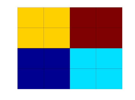
2x2 partition of a 4x4 Cartesian grid¶

To define a coarse grid, we must first compute a partition. To this end, we use partitionCartGrid, which exploits the logical structure and creates a uniform partitioning in logical space.

G = computeGeometry(cartGrid([4,4]));
p = partitionCartGrid(G.cartDims, [2,2]);
plotPartition(G, p);
colormap(jet), axis tight off

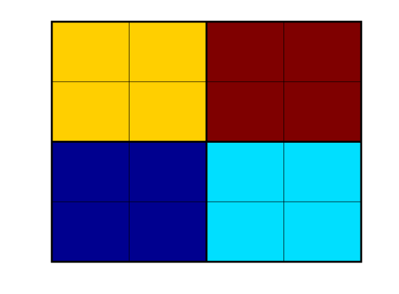
Generate coarse-grid structure¶

We can then call the routine that builds the structure representing the coarse grid. As a naming convention, we usually call this grid CG. The coarse grid can be passed on to any plotting routine in MRST. By calling coarsenGeometry on a grid which has been returned from processGeometry, we can get coarse centroids, volumes and so on.

CG = generateCoarseGrid(G, p);
CG = coarsenGeometry(CG);

cla
plotCellData(CG, (1:CG.cells.num)', 'EdgeColor','w','EdgeAlpha',.5);
plotFaces(CG, (1:CG.faces.num)', 'FaceColor','none','LineWidth', 2);

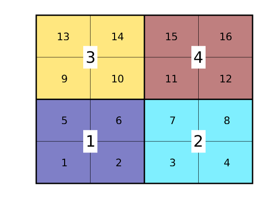
Show cell/block indices¶

In its basic form, the structure only represents topological information that specifies the relationship between blocks and block interfaces, etc. The structure also contains information of the underlying fine grid. Let us start by plotting cell/block indices

tg = text(G.cells.centroids(:,1), G.cells.centroids(:,2), ...
   num2str((1:G.cells.num)'),'FontSize',16, 'HorizontalAlignment','center');
tcg = text(CG.cells.centroids(:,1), CG.cells.centroids(:,2), ...
   num2str((1:CG.cells.num)'),'FontSize',24, 'HorizontalAlignment','center');
axis off;
set(tcg,'BackgroundColor','w','EdgeColor','none');
colormap(.5*jet+.5*ones(size(jet)));

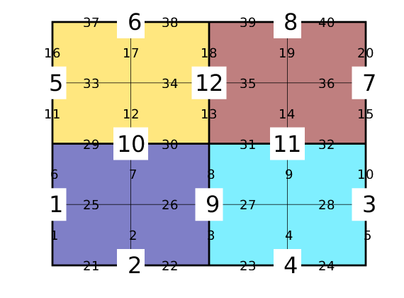
Show face indices of fine/coarse grids¶

delete([tg; tcg]);
tg = text(G.faces.centroids(:,1), G.faces.centroids(:,2), ...
   num2str((1:G.faces.num)'),'FontSize',14, 'HorizontalAlignment','center');
tcg = text(CG.faces.centroids(:,1), CG.faces.centroids(:,2), ...
   num2str((1:CG.faces.num)'),'FontSize',24, 'HorizontalAlignment','center');
set(tcg,'BackgroundColor','w','EdgeColor','none');

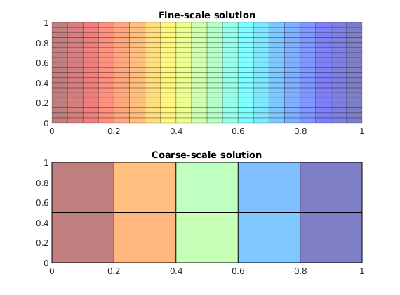
Solvers using coarse grids¶

The coarse grid will in most aspects behave as the standard grids and can be used in many of the solvers in MRST. Utilities such as ‘coarsenBC’ makes it easier to solve problems at several scales.

rstModule add incomp;

% Make a somewhat larger grid
G  = cartGrid([20, 20], [1 1]);
G  = computeGeometry(G);
p  = partitionCartGrid(G.cartDims,[5 2]);
CG = generateCoarseGrid(G, p);
CG = coarsenGeometry(CG);

% Trivial fluid
fluid = initSingleFluid('mu', 1, 'rho', 1);

% Uniform permeability and a pressure drop
rock.perm = ones(G.cells.num, 1);
T = computeTrans(G, rock);
state = initState(G, [], 0);
bc = pside([], G, 'left', 100*barsa);
bc = pside(bc, G, 'right', 0*barsa);

% Solve for fine scale
state = incompTPFA(state, G, T, fluid, 'bc', bc);

% Create the same trivial permeability for the coarse grid. This could be
% replaced by for example an upscaling routine from the upscaling module if
% the permeability was non-uniform.
rock.perm = ones(CG.cells.num, 1);
T_coarse = computeTrans(CG, rock);
state_coarse = initState(CG, [], 0);

% Take the existing boundary condition and sample it in the coarse grid.
bc_coarse = coarsenBC(CG, bc);
state_coarse = incompTPFA(state_coarse, CG, T_coarse, fluid, 'bc', bc_coarse);

% Plot the solutions
subplot(2,1,1)
plotCellData(G, state.pressure,'EdgeColor','k','EdgeAlpha',.2)
title('Fine-scale solution')
subplot(2,1,2)
plotCellData(CG, state_coarse.pressure,'EdgeColor','none')
plotFaces(CG,(1:CG.faces.num)','FaceColor','none');
title('Coarse-scale solution')

% <html>
% <p><font size="-1

Second Coarse-Grid Tutorial: Partitioning More Complex Grids¶

Generated from coarsegridExample2.m

In this tutorial, we will take a look at how to partition grids that have more complex geometries than the simple 2D grids we used in the first tutorial.

mrstModule add coarsegrid;

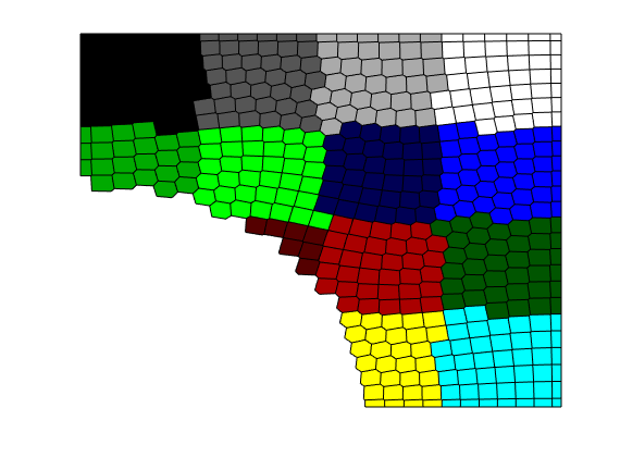
Partition a Non-rectangular 2D Grid¶

If the grid indices do not form a logical rectangle, we need to use the function ‘partitionUI’, which computes a uniform partition of the bounding box of the grid. To illustrate, we consider a rectilinear grid with a semi-circular cut-out along the lower edge.

dx = 1-0.5*cos((-1:0.1:1)*pi);
x = -1.15+0.1*cumsum(dx);
y = 0:0.05:1;
G = computeGeometry(tensorGrid(x, y.^.75));
r = sqrt(sum(G.cells.centroids.^2,2));
G = extractSubgrid(G, r>0.6);

clf
CG = generateCoarseGrid(G, partitionUI(G,[5 4]));
plotCellData(CG,(1:CG.cells.num)','EdgeColor','w','EdgeAlpha',.2);
plotFaces(CG,(1:CG.faces.num)', 'FaceColor','none','LineWidth',2);
colormap(.5*(colorcube(20) + ones(20,3))); axis off

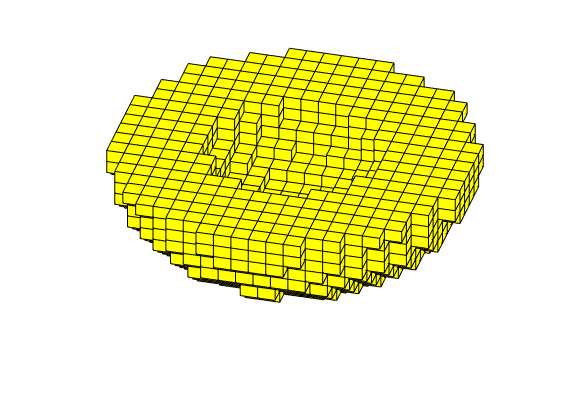
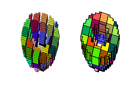
Partitioning a Cup-Formed Grid¶

3D Cartesian grid can be partitioned in the exact same way as 2D rectangular grids, using partitionCartGrid for grids that completely fill a hexahedron and partitionUI for grids that do not. As an illustration, we will partition a domain formed as a cup

clf
x = linspace(-2,2,41);
G = tensorGrid(x,x,x);
G = computeGeometry(G);
c = G.cells.centroids;
r = c(:,1).^2 + c(:,2).^2+c(:,3).^2;
G = removeCells(G, (r>1) | (r<0.25) | (c(:,3)<0));
plotGrid(G); view(15,60); axis tight off

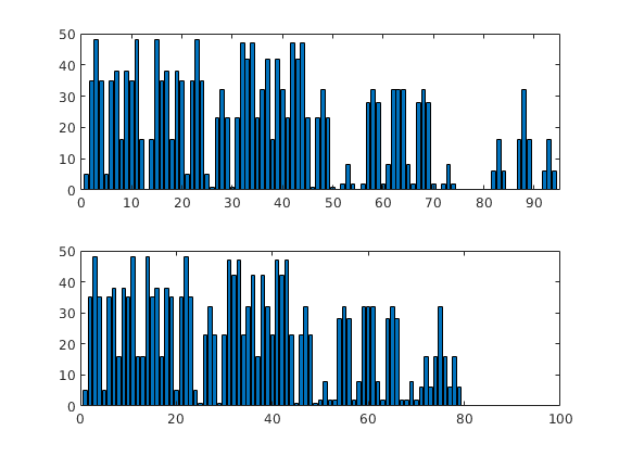
Since the grid only covers subregion of its bounding box, the partition vector will not be contiguous. To avoid having to treat special cases arising from non-contigous partition vectors, most routines in MRST require partition vectors to be contiguous. To get a contigous partition vector, we use the function ‘compressPartition’

clf
p = partitionUI(G,[5 5 4]);
subplot(2,1,1); bar(accumarray(p,1)); shading flat
q = compressPartition(p);
subplot(2,1,2); bar(accumarray(q,1)); shading flat
set(gca,'XLim',[0 100]);

And then we are ready to make the coarse grid. The figure below shows two different ways of visualizing the grid

CG = generateCoarseGrid(G, q);

subplot(1,2,1)
explosionView(G,q,.4);
view(15,60); axis tight off
colormap(colorcube(max(q)));

subplot(1,2,2)
plotCellData(CG,(1:CG.cells.num)','EdgeColor','w','EdgeAlpha',.2);
plotFaces(CG,(1:CG.faces.num)', 'FaceColor','none','LineWidth',2);
view(15,60); axis tight off

Partitioning an Unstructured Grid¶

The same principle applies to unstructured grids. So let us try to partition a Voronoi grid into a semi-rectangular coarse grid. The function partitionUI only works for fine grids with an underlying Cartesian topography, so we can rely on the function ‘sampleFromBox’ which uses the cell centroids to sample from a uniform Cartesian grid covering the bounding box of the grid

[x,y] = meshgrid(linspace(0,1,25));
pt = twister([x(:) y(:)]);
G = pebi( triangleGrid(pt, delaunay(pt)));
G = computeGeometry(G);
r = sqrt(sum(G.cells.centroids.^2,2));
G = extractSubgrid(G, r>0.6);
p = sampleFromBox(G, reshape(1:16,4,4));
clf
plotCellData(G,p); colormap(colorcube(16)); axis tight off

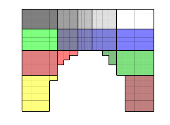
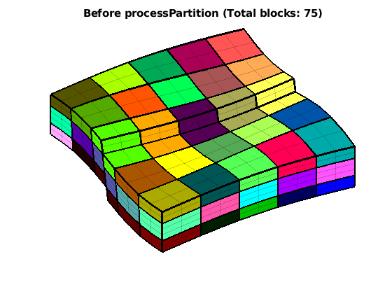
Create a faulted grid and partition it¶

We create a grid and partition it logically in ij-space and along specific layers along the k-space.

rdecl = simpleGrdecl([10 10 7], .15);
G = computeGeometry( processGRDECL(grdecl) );
% Layer 1 will go from 1 to 3 - 1, layer 2 from 3 to 6 - 1 and so on
L = [1 3 6 8];
% We can easily find the thickness of the layers
diff(L)

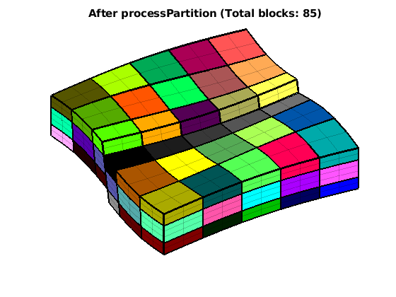
% The partition is disconnected across the fault. processPartition can
% amend this by adding new coarse blocks.
p_initial = partitionLayers(G, [5,5], L);
p = processPartition(G, p_initial); mp = max(p);

figure
CGi = generateCoarseGrid(G,p_initial);
plotCellData(G, p_initial, 'EdgeAlpha', .2);
plotFaces(CGi,(1:CGi.faces.num),'FaceColor','none','EdgeColor','w','LineWidth',2);
title(['Before processPartition (Total blocks: ' num2str(max(p_initial)) ')'])
view(60,65); colormap(colorcube(mp)); caxis([1 mp]); axis tight off

figure
CG = coarsenGeometry( generateCoarseGrid(G,p) );
plotCellData(G, p, 'EdgeAlpha', .2);
plotFaces(CG,(1:CG.faces.num),'FaceColor','none','EdgeColor','w','LineWidth',2);
title(['After processPartition (Total blocks: ' num2str(mp) ')'])
view(60,65); colormap(colorcube(mp)); caxis([1 mp]); axis tight off

% <html>
% <p><font size="-1

ans =

     2     3     2

More About Coarsegrid Geometry/Topology¶

Generated from coarsegridExample3.m

In this example, we will take a closer look at ways of working with the geometry and topology of the coarse grids

mrstModule add coarsegrid

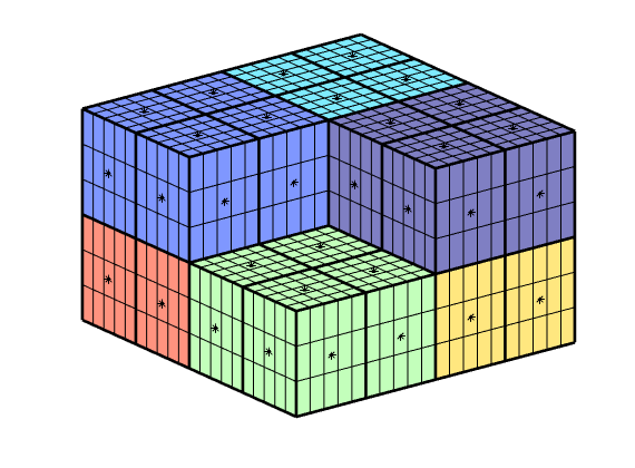
Subdivision of Coarse Faces¶

So far, we have assumed that there is only a single connection between two neighboring coarse blocks. This connection is built up of all faces between pairs of fine cells that belong to the two different coarse blocks. However, we can make coarse grids that have multiple connections between neighboring grid blocks, as the following examples shows.

G = computeGeometry(cartGrid([20 20 6]));
c = G.cells.centroids;
G = removeCells(G, (c(:,1)<10) & (c(:,2)<10) & (c(:,3)<3));

p = partitionUI(G,[2, 2, 2]); p = compressPartition(p); mp = max(p);
q = partitionUI(G,[4, 4, 2]);
CG = generateCoarseGrid(G, compressPartition(p), ...
                        cellPartitionToFacePartition(G,q));
clf
plotCellData(CG,(1:mp)');
plotFaces(CG,1:CG.faces.num,'FaceColor' , 'none' , 'LineWidth' ,2);
view(3); axis off
colormap(.5*(jet(128)+ones(128,3)));

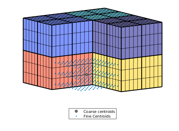
Adding geometry information to the coarse grid¶

Unlike the fine grids, the coarse grid structure only contains topological information by default. This means, in particular, that coarse grids do not have nodes. By calling coarsenGeometry, we can get coarse block and face centroids, volumes, and so on.

CG = coarsenGeometry(CG);

plotPts = @(pts, varargin) plot3(pts(:,1), pts(:,2), pts(:,3), varargin{:});
hold on
h=plotPts(CG.faces.centroids, 'k*');
hold off;

Let us look more in detail on the relationship between centroids in the fine and coarse grid

i = false(mp,1); i(4) = true;
cla, hold
cg_cent = CG.cells.centroids(i,:);   plotPts(cg_cent, 'ok','MarkerFaceColor',[.5 .5 .5]);
g_cent = G.cells.centroids(p==4,:);  plotPts(g_cent, '.');
plotCellData(CG,(1:mp)',~i);
plotFaces(CG,gridCellFaces(CG,find(~i)),'FaceColor','none','LineWidth',2);
view(-35,15);
legend({'Coarse centroids', 'Fine Centroids'}, 'Location', 'SouthOutside')

Current plot held

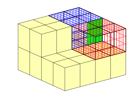
The coarse grid also contains lookup tables for mapping blocks and interfaces in the coarse grid to cells and faces in the fine grid. To demonstrate this, we visualize a single coarse face consisting of several fine faces along with the cells its block neighbors in red and blue respectively on the fine grid.

ace  = 66;
sub   = CG.faces.connPos(face):CG.faces.connPos(face+1)-1;
ff    = CG.faces.fconn(sub);
neigh = CG.faces.neighbors(face,:);

clf
show = false(1,CG.faces.num);
show(boundaryFaces(CG)) = true;
show(boundaryFaces(CG,neigh)) = false;
plotFaces(CG, show,'FaceColor',[1 1 .7]);
plotFaces(CG,boundaryFaces(CG,neigh),'FaceColor','none','LineWidth', 2);
plotFaces(G, ff, 'FaceColor', 'g')
plotGrid(G, p == neigh(1), 'FaceColor', 'none', 'EdgeColor', 'r')
plotGrid(G, p == neigh(2), 'FaceColor', 'none', 'EdgeColor', 'b')
view(3); axis off

% <html>
% <p><font size="-1

More about partition vectors¶

Generated from coarsegridExample4.m

In this tutorial, we will take a closer look at partition vectors and discuss how different types of partitions can be combined into one.

mrstModule add coarsegrid

Partition according to polar coordinate¶

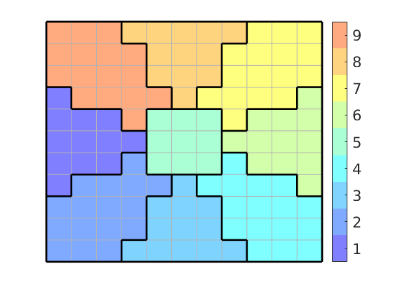
In the first example, we partition the box [-1,1]x[-1,1] into nine different blocks using the polar coordinates of the cell centroids. The first block is defined as r<=.3, while the remaining eight are defined by segmenting 4 theta/pi:

clf
G = cartGrid([11, 11],[2,2]);
G.nodes.coords = bsxfun(@minus, G.nodes.coords, 1);
G = computeGeometry(G);
c = G.cells.centroids;
[th,r] = cart2pol(c(:,1),c(:,2));
p = mod(round(4*th/pi)+4,4)+1;
p(r<.3) = max(p)+1;

plotCellData(G,p,'EdgeColor',[.7 .7 .7]);
outlineCoarseGrid(G,p,'k');
caxis([.5 max(p)+.5]);
colormap(.5*(jet(max(p))+ones(max(p),3)));
set(colorbar,'YTick',1:max(p),'FontSize',16);
axis off

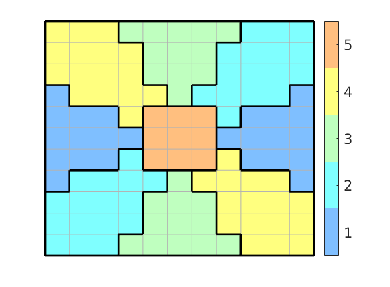
In the figure it is simple to distinguish nine different coarse blocks, but since we only have five colors, there are actually five blocks. Four of these are disconnected in the sense that they contain cells that cannot be connected by a path that only crosses faces between cells inside the block. We use the routine ‘processPartition’ to split these blocks

p = processPartition(G, p);
figure
plotCellData(G,p,'EdgeColor',[.7 .7 .7]);
outlineCoarseGrid(G,p,'k');
caxis([.5 max(p)+.5]);
colormap(.5*(jet(max(p))+ones(max(p),3)));
set(colorbar,'YTick',1:max(p),'FontSize',16);
axis off

No need for logical indices¶

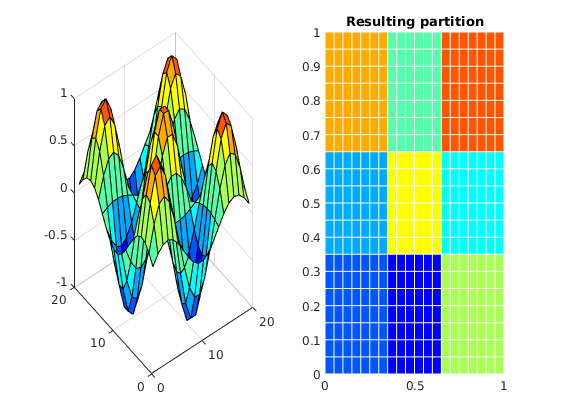
As you have seen in the previous example, the partition vector is just a vector that tells the index of the block a given cell belongs to. This means that we can generate an arbitrary coarse grid without using any information relating to the geometry or topology of the grid. For instance, if we want to partition a grid uniformly in space based on cell coordinates, the product of two periodic functions will do nicely. To illustrate this, we can divide a rectangular grid into a 3x3 coarse grid by exploiting that the sine function changes sign in intervals of pi.

nx = 3; ny = 3;
G = computeGeometry(cartGrid([20, 20], [1 1]));

% First create the periodic function
f = @(v) sin(pi*nx*v(:,1)) .* sin(pi*ny*v(:,2));
% Evaluate it in the centroids
fval = f( G.cells.centroids);

% We divide the grid into two parts based on the sign of the function
% and postprocess to create connected domains.
p = double(fval > 0) + 1;
p = processPartition(G, p);

% This vector can generate coarse grids just as partitionUI did.
CG = generateCoarseGrid(G, p);
clf
subplot(1,2,1); title('f(x)')
v = reshape(f(G.cells.centroids), G.cartDims(1), G.cartDims(2));
surf(v)

subplot(1,2,2); title('Resulting partition')
plotCellData(G, mod(p, 13), 'EdgeColor', 'w');
colormap(jet)

Combining multiple partition vectors¶

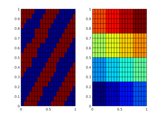
A very efficient way to generate coarse partitions is to combine two or more partition vectors that each implement a coarsening principle. As an examples, let us consider a case where our geological model contains two different facies. We can use this information, together with a standard partition, to make a coarse grid that adapts to the geology in the sense that we only get coarse blocks that contain a single facies. This could, for instance, be important when upscaling properties that are very different.

clf

% Make a diagonal and periodic facies distribution
f  = @(c) sin(4*pi*(c(:,1)-c(:,2)));
pf = 1 + (f(G.cells.centroids) > 0);
subplot(1,2,1);plotCellData(G,pf); view(2);

% Make a rectangular coarse partition
pc = partitionCartGrid(G.cartDims, [4 4]);
subplot(1,2,2), plotCellData(G,pc); view(2); colormap(jet(128));

Alternative 1: Collect the partitions as columns in an array and the use ‘unique’ to find all unique combinations. These will give the intersection of the two. This technique can be generalized to an arbitrary number of partition vectors, but is costly since ‘unique’ performs a search.

tic, [b,~,p] = unique([pf, pc], 'rows' ); toc

Elapsed time is 0.000545 seconds.

Alternative 2: We can treat the partition vectors as multiple subscripts, and use this to compute a linear index. This index will not be contiguous and thus needs to be compressed. This method is fast, but more difficult to extend to multiple partition vectors using a single statement.

tic, q = compressPartition(pf + max(pf)*pc); toc

Elapsed time is 0.000555 seconds.

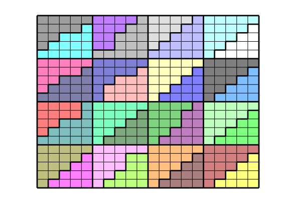
Plot the resulting grid

igure
plotCellData(G,p);
outlineCoarseGrid(G, p, 'k','LineWidth',2);
axis off
mp = max(p);
colormap(.5*(colorcube(mp)+ones(mp,3)))

% <html>
% <p><font size="-1

Coarsening the Norne Simulation Model¶

Generated from coarsegridExampleNorne.m

We show how to coarsen the simulation model of the Norne field by partitioning it uniformly in logical Cartesian space. We visualize some of the coarse blocks and show how they are connected with their neighbors.

mrstModule add coarsegrid

Read and process model¶

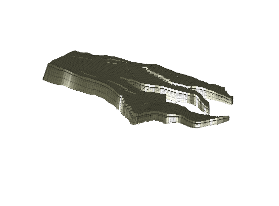
The Norne model is one of the standard data sets that have been used a lot with MRST. Unfortunately, you have to download the model manually. How to do this, can be found by typing getDatasetInfo('norne'). We pick the part of the model that represents the main reservoir and disregard the stack of twelve cells that are disconnected from the rest of the model.

dpath  = getDatasetPath('norne');
grdecl = fullfile(dpath, 'NORNE.GRDECL');
grdecl = readGRDECL(grdecl);
G = processGRDECL(grdecl);
G = computeGeometry(G(1));

clf,
plotGrid(G,'EdgeAlpha',.1,'FaceColor',[.9 .9 .7]);
view(70,70), zoom(2), axis tight off
set(gca,'Zdir','normal'); camlight headlight; set(gca,'Zdir','reverse');

Partition the grid in logical space¶

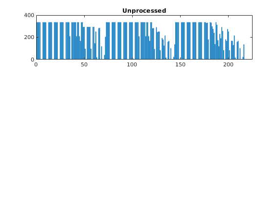
To construct a coarse grid, we try to partition the grid uniformly as 6x12x3 coarse blocks in index space. This will partition all cells in the logical 46x112x22 grid, including cells that are inactive. The number of active cells within each coarse block is shown in the bar plot below.

p = partitionUI(G,[6 12 3]);
newplot, subplot(3,1,1)
bar(accumarray(p,1)); set(gca,'XLim',[0 225]);
title('Unprocessed');

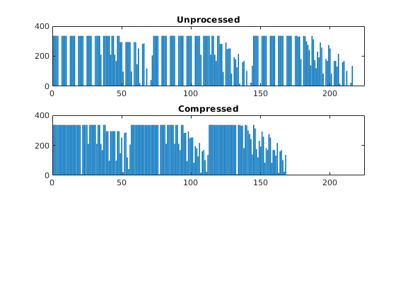
As we can see from the bar plot, there are several coarse block that contain no active cells. We therefore postprocess the partitioning to remove blocks that contain no active cells, and then renumber the overall partitioning, giving a new total of 168 blocks.

p = compressPartition(p); max(p)
subplot(3,1,2)
bar(accumarray(p,1)); set(gca,'XLim',[0 225]);
title('Compressed');

ans =

   168

Because the partitioning has been performed in logical index space, we have so far disregarded the fact the some of the blocks may contain disconnected cells because of erosion, faults, etc. We therefore postprocess the grid in physical space and split disconnected blocks.

p = processPartition(G,p); m=max(p);
subplot(3,1,3)
bar(accumarray(p,1)); set(gca,'XLim',[0 225]);
title('Processed');

assert (all(accumarray(p, 1) > 0))

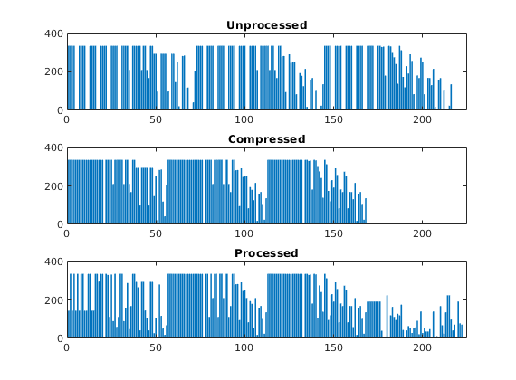
We have now obtained a partitioning consisting of 223 blocks, in which each coarse block consists of a set of connected cells in the fine grid. To show the partitioning, we plot the coarse blocks using a random and cyclic color scheme for the blocks.

newplot
subplot('position',[0.025 0.025 0.95 0.95])
plotCellData(G,p,'EdgeAlpha',.5);
axis tight off; view(0,75), colormap(colorcube(m));

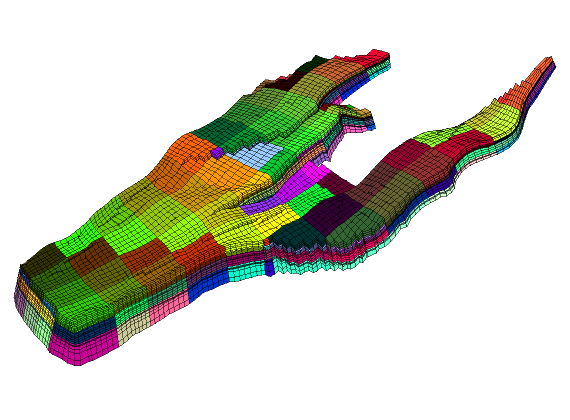
From the plot above, it is not easy to see the shape of the individual coarse blocks. In the next section, we will therefore show some examples of how individual blocks can be visualized.

Build the coarse-grid¶

Having obtained a partition we are satisfied with, we build the coarse-grid structure. This structure consists of three parts:

CG = generateCoarseGrid(G, p);
CG             %#ok<NOPTS> (intentional display)
CG.cells       %  (intentional display)
CG.faces       %  (intentional display)

CG =

  struct with fields:

        cells: [1×1 struct]
        faces: [1×1 struct]
    partition: [44915×1 double]
...

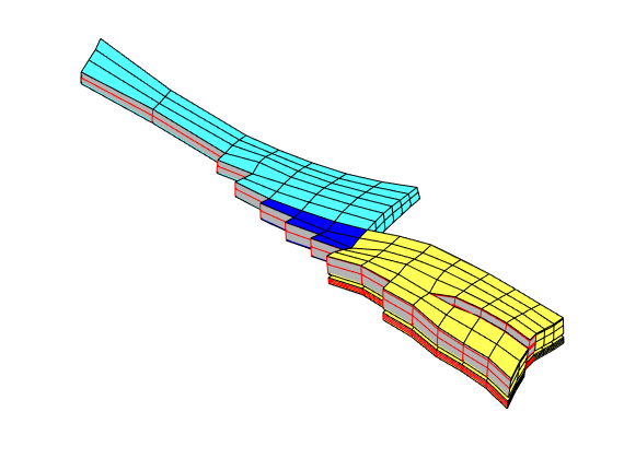
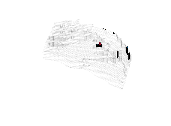
Let us now use CG to inspect some of the blocks in the coarse grid. To this end, we arbitrarily pick a few blocks and inspect these block and their neighbours. For the first block, we plot the cells and the faces that have been marked as lying on a fault

clf, plotBlockAndNeighbors(CG, 55), view(-90,70)

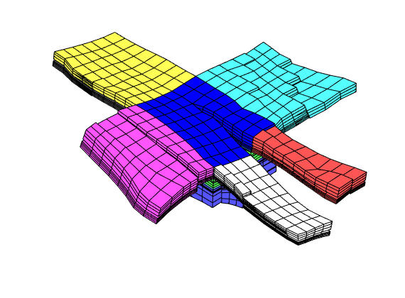
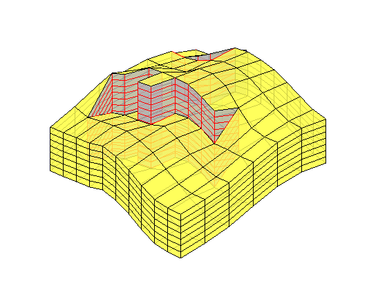
For the second block, we only plot the cells and not the faulted faces

clf
plotBlockAndNeighbors(CG, 19, 'PlotFaults', false([2, 1]))
view(90, 70)

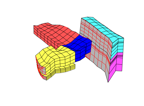
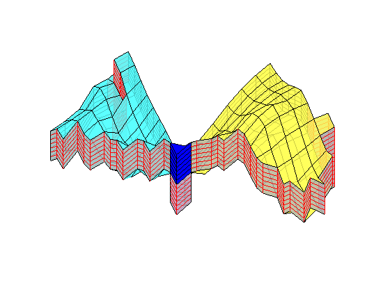
The third set of neighboring blocks contains more faults

clf, plotBlockAndNeighbors(CG, 191), view(100, 30)

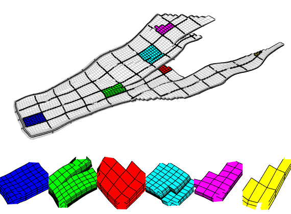
We end the example by highlight six representative blocks, including the three blocks we inspected above. Notice that this way of visualization only uses the fine grid and the partition vector, and thus does not require that the coarse-grid structure has been built.

clf
blocks = [3, 19, 191, 34, 196, 55];
col = ['b', 'g', 'r', 'c', 'm', 'y'];
axes('position', [0.01, 0.25, 0.99, 0.75]);
plotGrid(G, 'EdgeColor', [0.75, 0.75, 0.75], 'FaceColor', 'w');
outlineCoarseGrid(G, p, 'FaceColor', 'none', 'LineWidth', 2);

for i = 1 : 6,
   plotGrid(G, p == blocks(i), 'FaceColor', col(i));
end
axis tight off, view(10, 90)

% Plot the chosen 6 coarse blocks
for i = 1 : 6,
   axes('position', [(i-1)/6, 0.02, 1/6, 0.25]);

   plotGrid(G, p == blocks(i), 'FaceColor', col(i));

   axis tight off, view(0,75), zoom(1.2)
end

<html>
% <p><font size="-1

Coarsening the SAIGUP Model¶

Generated from coarsegridExampleSAIGUP.m

We show how to coarsen the SAIGUP model by partitioning it uniformly in logical Cartesian space. We visualize some of the coarse blocks and show how they are connected with their neighbors.

mrstModule add coarsegrid

Read and process model¶

The SAIGUP model is one of the standard data sets provided with MRST. We therefore check if it is present, and if not, download and install it.

pth    = getDatasetPath('SAIGUP');
grdecl = fullfile(pth, 'SAIGUP.GRDECL');
grdecl = readGRDECL(grdecl);
G = processGRDECL(grdecl);
G = computeGeometry(G);

Partition the grid in logical space¶

We construct a coarse grid by partitioning the grid uniformly as 6x12x3 coarse blocks in index space. This process partitions all cells in the logical 40x120x20 grid, including cells that are inactive. We therefore compress the partitioning to remove blocks that contain no active cells, and then renumber the overall partitioning. Some of the blocks may contain disconnected cells because of erosion, faults, etc. We therefore postprocess the grid in physical space and split disconnected blocks.

p = partitionUI(G,[6 12 3]);
p = compressPartition(p);
p = processPartition(G,p);
assert (all(accumarray(p, 1) > 0))

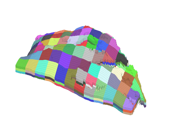
We have now obtained a partitioning consisting of 243 blocks, in which each coarse block consists of a set of connected cells in the fine grid. To show the partitioning, we plot the coarse blocks using a random permutation of the block numbers.

newplot
subplot('position',[0.025 0.025 0.95 0.95]);
m = max(p);
q = randperm(m)';
plotCellData(G,q(p),'EdgeAlpha',0.1);
set(gca,'dataasp',[15 15 2])
axis tight off; view(-60,40);
cmap = .7*colorcube(m)+.3*ones(m,3); colormap(cmap);

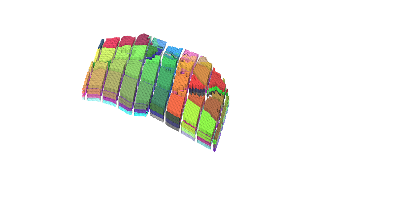
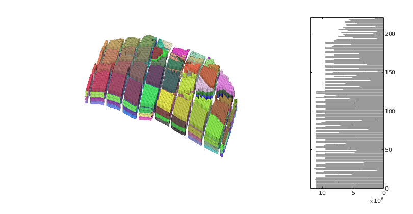
Alternatively, we can use the explosion technique

figure('Position',[0 60 800 420]);
axes('Position',[.01 .11 .775 .81]);
explosionView(G, p, 'EdgeAlpha', .1);
axis tight off; set(gca,'DataAspect',[1 1 0.1]);
view(-65,55); zoom(1.4); camdolly(0,-0.2,0)
colormap(cmap);

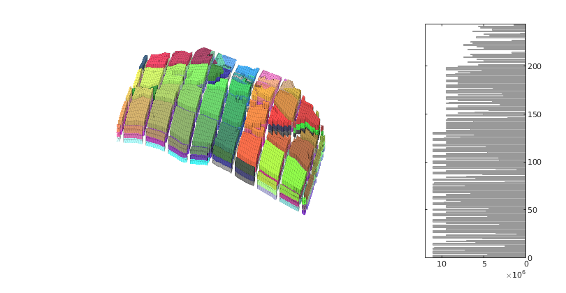
Build the coarse-grid and inspect the distribution of block volumes¶

The original fine-scale model has the peculiar characteristic that all cells have the same size. In the coarsened model there is almost two orders difference between the smallest and largest blocks.

CG = generateCoarseGrid(G, p); P=p;
CG = coarsenGeometry(CG);

axes('Position',[.75 .12 .18 .8]);
h = barh(CG.cells.volumes,'b');
set(gca,'xdir','reverse','YAxisLocation','right',...
   'Fontsize',8,'XLim',[0 12]*1e6);
set(h,'FaceColor',[.7 .7 .7],'EdgeColor',[.6 .6 .6]);

To get a more even size distribution for the coarse blocks, we will remove some of the smallest blocks by merging them with the neighbor that has the smallest block volume. This is done repeatedly until the volumes of all blocks are above a certain lower threshold. First, we visualize all blocks that have volume less than ten percent of the mean block volume.

blockVols = CG.cells.volumes;
meanVol   = mean(blockVols);
show = blockVols<.1*meanVol;
figure
plotGrid(G,'FaceColor','none','EdgeAlpha',.05);
bcol = zeros(max(p),1); bcol(show)=1:sum(show);
plotCellData(CG,bcol, show);
axis tight off; set(gca,'DataAspect',[1 1 0.1]);
view(-65,55); zoom(1.4); camdolly(0,-0.2,0)
colormap(lines);

The merging algorithm is quite simple: we compute the block volumes, select the block with the smallest volume, and then merge this block with one of its neighbors, depending on some criterion (e.g., the neighbor with the largest or smallest block volume). Then we update the partition vector by relabling all cells in the block with the new block number, compress the partition vector to get rid of empty entries, regenerate a coarse grid, recompute block volumes, pick the block with the smallest volume in the new grid, and so on. In each iteration, we plot the selected block and its neighbors.

[minVol, block] = min(blockVols);
i = 1;
while minVol<.1*meanVol
   % Find all neighbors of the block
   clist = any(CG.faces.neighbors==block,2);
   nlist = reshape(CG.faces.neighbors(clist,:),[],1);
   nlist = unique(nlist(nlist>0 & nlist~=block));

   % Alt 1: merge with neighbor having smallest volume
   % [~,merge] = min(blockVols(nlist));

   % Alt 2: sort neigbors by cell volume and merge with the one in the
   % middle
   % [~,ind] = sort(blockVols(nlist),1,'descend');
   % merge = ind(round(numel(ind)/2));

   % Alt 3: merge with neighbor having largest volume
   [~,merge] = max(blockVols(nlist));

   % Only plot three selected examples
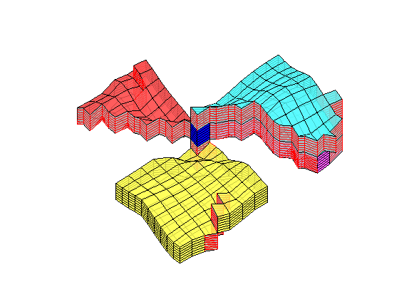
   if ismember(i,[12,13,15])
      figure;
      plotBlockAndNeighbors(CG, block, ...
         'PlotFaults', [false, true], 'Alpha', [1 .8 .8 .8]);
   end

   % Update partition vector
   p(p==block)  = nlist(merge);
   p = compressPartition(p);

   % Regenerate coarse grid and pick the block with the smallest volume
   CG = generateCoarseGrid(G, p);
   CG = coarsenGeometry(CG);
   blockVols = CG.cells.volumes;
   [minVol, block] = min(blockVols);
   i = i+1;
end

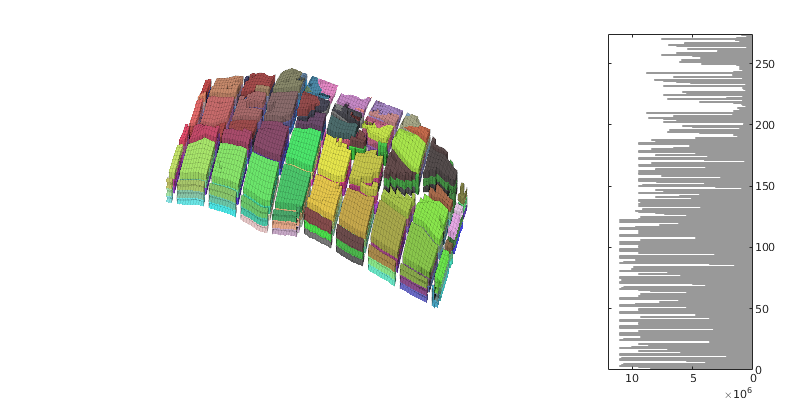
Make new plot with the revised coarse grid

figure('Position',[0 60 800 420]);
axes('Position',[.01 .11 .775 .81]);
explosionView(G, CG.partition, 'EdgeAlpha', .1);
axis tight off; set(gca,'DataAspect',[1 1 0.1]);
view(-65,55); zoom(1.4); camdolly(0,-0.2,0)
colormap(.3*(2*colorcube(CG.cells.num)+ones(CG.cells.num,3)));

axes('Position',[.75 .12 .18 .8]);
h = barh(CG.cells.volumes,'b');
set(gca,'xdir','reverse','YAxisLocation','right',...
   'Fontsize',8,'XLim',[0 12]*1e6);
set(h,'FaceColor',[.7 .7 .7],'EdgeColor',[.6 .6 .6]);

In the partition above, there were several blocks that were only connected through small face areas in their interior. To try to improve this problem, we recompute the partitioning, but now disregard couplings across small faces when postprocessing the initial, uniform partition

p = partitionUI(G,[6 12 3]);
p = compressPartition(p);
p = processPartition(G, p, G.faces.areas<250);
CG1 = generateCoarseGrid(G,p);
CG1 = coarsenGeometry(CG1);

The next step is to redo the merging of small blocks. The algorithm used above was written to make the visualization of the changing grid as simple as possible. The implementation is not very efficient since we in each step regenerate the coarse grid and compute all the block volumes. This time, we will use another implementation that is a bit more involved, but also more efficient.

blockVols       = CG1.cells.volumes;
meanVol         = mean(blockVols);
newBlockList    = 1:max(p);
[minVol, block] = min(blockVols);
while minVol<.1*meanVol
   nlist = reshape(CG1.faces.neighbors(any(CG1.faces.neighbors==block,2),:),[],1);
   nlist = newBlockList(nlist(nlist>0));
   nlist = unique(nlist(nlist~=block));

   [nVol,merge] = min(blockVols(nlist));

   newBlockNo   = nlist(merge);
   p(p==block)  = newBlockNo;
   newBlockList(block)   = newBlockNo;
   blockVols(block)      = inf;
   blockVols(newBlockNo) = minVol + nVol;

   [minVol, block] = min(blockVols);
end
p = compressPartition(p);
CG1 = generateCoarseGrid(G, p);
CG1 = coarsenGeometry(CG1);

Make new plot with the revised coarse grid

figure('Position',[0 60 800 420]);
axes('Position',[.01 .11 .775 .81]);
explosionView(G, CG1.partition, 'EdgeAlpha', .1);
axis tight off; set(gca,'DataAspect',[1 1 0.1]);
view(-65,55); zoom(1.4); camdolly(0,-0.2,0)
colormap(.3*(2*colorcube(CG1.cells.num)+ones(CG1.cells.num,3)));

axes('Position',[.75 .12 .18 .8]);
h = barh(CG1.cells.volumes,'b');
set(gca,'xdir','reverse','YAxisLocation','right',...
   'Fontsize',8,'XLim',[0 12]*1e6);
set(h,'FaceColor',[.7 .7 .7],'EdgeColor',[.6 .6 .6]);

<html>
% <p><font size="-1

coarsegrid: Generation of coarse grids¶

Utilities¶

Plotting¶

Examples¶

Introduction to Coarse Grids in MRST¶

2x2 partition of a 4x4 Cartesian grid¶

Generate coarse-grid structure¶

Show cell/block indices¶

Show face indices of fine/coarse grids¶

Solvers using coarse grids¶

Second Coarse-Grid Tutorial: Partitioning More Complex Grids¶

Partition a Non-rectangular 2D Grid¶

Partitioning a Cup-Formed Grid¶

Partitioning an Unstructured Grid¶

Create a faulted grid and partition it¶

More About Coarsegrid Geometry/Topology¶

Subdivision of Coarse Faces¶

Adding geometry information to the coarse grid¶

More about partition vectors¶

Partition according to polar coordinate¶

No need for logical indices¶

Combining multiple partition vectors¶

Coarsening the Norne Simulation Model¶

Read and process model¶

Partition the grid in logical space¶

Build the coarse-grid¶

Coarsening the SAIGUP Model¶

Read and process model¶

Partition the grid in logical space¶

Build the coarse-grid and inspect the distribution of block volumes¶

`coarsegrid`: Generation of coarse grids¶