msrsb: Multiscale Restriction-Smoothed Basis method for pressure

Implementation of the Multiscale Restricted-Smoothing Basis (MsRSB) method. MsRSB is a very robust and versatile multiscale method that can either be used as an approximate coarse-scale solver having mass-conservative subscale resolution, or as an iterative fine-scale solver that will provide mass-conservative solutions for any given tolerance.

Utilities

Contents

MSRSB

Files

getMultiscaleBasis - Get multiscale basis functions for a given coarse grid and system matrix incompMultiscale - Solve incompressible TPFA flow problem using approximate multiscale method

getMultiscaleBasis(CG, A, varargin)

Get multiscale basis functions for a given coarse grid and system matrix

Synopsis:

[basis, CG] = getMultiscaleBasis(CG, A, 'type', 'msfv')

Parameters:

• CG – Coarse grid.
• A – System matrix for which the basis functions are to be computed.

Keyword Arguments:  

• type – Type of basis functions. Available options are ‘MsRSB’ for basis functions based on restricted smoothing and ‘MsFV’ for basis functions based on localized flow problems and a dual grid.
• regularizeSys – Regularize system before computing basis functions, by ensuring that the row and column sum of the matrix is zero. Default on.
• iterations – Max number of iterations in MsRSB basis functions. No effect on other solvers.
• tolerance – Tolerance for MsRSB basis functions.
• implicitDual – Indicator if the MsFV basis functions are generated with implicit or explicit dual grid. Implicit generally makes it easier to generate dual grids, but the basis construction is no longer local in nature for complex grids.
• useControlVolume – Use a control volume restriction operator, required for flux reconstruction. If disabled, will set R = B^T, i.e. Galerkin/finite element type which will give better iterative convergence if the coarse scale stencil is unstable.

Returns:

basis – Struct suitable for incompMultiscale. Contains fields .B for basis functions and .R for the restriction operator as well as the name of the method in .type.

See also

incompMultiscale

incompMultiscale(state, CG, T, fluid, basis, varargin)

Solve incompressible TPFA flow problem using approximate multiscale method

Synopsis:

[state, report] = incompMultiscale(state, CG, T, fluid, basis)

Description:

This function supports the same types of problems as incompTPFA. Requires precomputed basis and coarsegrids. Supports flux reconstruction and iterative improvement of solution.

Parameters:

• state – See incompTPFA.
• CG – Coarsegrid used to generate basis functions
• T – See incompTPFA.
• fluid – See incompTPFA.
• basis – Basis functions from getMultiscaleBasis.

Keyword Arguments:  

• any – Additional options are passed onto incompTPFA.
• getSmoother – Smoother function from getSmootherFunction. Required if iterations is set to anything larger than zero.
• iterations – Number of multiscale iterations. Requires getSmoother option. Default option is zero, which means that the multiscale system will be solved a single time without any application of smoothers.
• tolerance – Tolerance for iterative solver. Interpreted as |A*x - b|_2 / |b|_2 <= tolerance for convergence.
• useGMRES – If enabled, GMRES will be used to accelerate the iterations.
• LinSolve – Linear solver function handle for coarse scale system. Typically only required if the coarse grid has several thousand blocks.
• reconstruct – If enabled, the solver will reconstruct a divergence-free velocity field suitable for transport. This is not required if the number of iterations is large enough that the pressure is completely resolved. Note that this requires that the restriction operator uses a control-volume form.

Returns:

• state – Solved reservoir state.
• report – Report from linear iterative solver.

Contents

UTILS

Files

addCoarseCenterPoints - Adds center points to each block. A center is typically the fine cell changeCoarseCenterToWellLocation - Designates coarse nodes to cells containing wells. For coarse blocks with controlVolumeRestriction - Control volume restriction operator for a given coarsegrid partition. eliminateWellEquations - Eliminate well equations from linear system formReconstructionMatrix - Form matrix for multiscale flux reconstruction getCellNeighbors - List of cell neighbors for a single cell. getEnclosingCellsByFace - Get cells enclosing a set of points using dot product with center-face getIncomp1PhMatrix - Get TPFA-like incompressible system matrix via incompTPFA. getSystemIncompTPFA - Extract linear system from two point solver without solving any linear mapCenters - Map fine cells as centers of coarse cells and faces. reconstructPressure - Solve reconstruction problem for multiscale methods recoverWellSolution - Recover previously eliminated well equations from solved system setCentersByWells - Small utility to set centers of coarse blocks to one of the well cells.

addCoarseCenterPoints(CG, varargin)

Adds center points to each block. A center is typically the fine cell closest to the geometrical centroid of the block.

changeCoarseCenterToWellLocation(CGm, W)

Designates coarse nodes to cells containing wells. For coarse blocks with multiple cells, it selects a random well location as coarse node

controlVolumeRestriction(partition)

Control volume restriction operator for a given coarsegrid partition.

eliminateWellEquations(A, q, nc)

Eliminate well equations from linear system

formReconstructionMatrix(A, partition, keepDiag)

Form matrix for multiscale flux reconstruction

getCellNeighbors(G, c)

List of cell neighbors for a single cell.

getEnclosingCellsByFace(G, pts, varargin)

Get cells enclosing a set of points using dot product with center-face vectors.

getIncomp1PhMatrix(G, T, state, fluid)

Get TPFA-like incompressible system matrix via incompTPFA.

getSystemIncompTPFA(state, G, T, fluid, varargin)

Extract linear system from two point solver without solving any linear systems.

mapCenters(CG, blockCenters, faceCenters)

Map fine cells as centers of coarse cells and faces.

reconstructPressure(partition, pressure, A, rhs, fixMethod)

Solve reconstruction problem for multiscale methods

recoverWellSolution(A_ww, A_wp, q_w, p)

Recover previously eliminated well equations from solved system

setCentersByWells(CG, W, varargin)

Small utility to set centers of coarse blocks to one of the well cells.

Contents

ACCELERATED

Files

boundaryNeighbors - cppMultiscaleBasis - Create MsRSB basis using MEX code cppMultiscaleBasisFromFile - mex_cppMultiscaleBasis - Internal build routine for MsRSB accelerated basis functions setupMexInteractionMapping - Setup mex mapping for cppMultiscaleBasis

cppMultiscaleBasis(CG, A, varargin)

Create MsRSB basis using MEX code

mex_cppMultiscaleBasis(varargin)

Internal build routine for MsRSB accelerated basis functions

setupMexInteractionMapping(CG, varargin)

Setup mex mapping for cppMultiscaleBasis

Contents

COARSEGRID

Files

basisToCoarseGrid - Create a coarse grid from a set of basis functions so that each coarse coarseNeighbors - Determine coarse neighbors for a given coarse cell (MPFA or TPFA-like). partitionUniformPadded - Equivialent to partitionUI from the coarsegrid module, with a small storeInteractionRegion - Store interaction region for coarse grid storeInteractionRegionCart - Store MPFA-like interaction region for coarse grid made from logical partitioning.

basisToCoarseGrid(G, I)

Create a coarse grid from a set of basis functions so that each coarse block corresponds to the places where that basis is the largest value.

coarseNeighbors(CG, cell, isMPFA, faceNodePos)

Determine coarse neighbors for a given coarse cell (MPFA or TPFA-like).

partitionUniformPadded(G, dims)

Equivialent to partitionUI from the coarsegrid module, with a small half-block at each end of the domain.

storeInteractionRegion(CG, varargin)

Store interaction region for coarse grid

Synopsis:

CG = storeInteractionRegion(CG);

Description:

Compute and store the interaction/support regions for coarse blocks. Each coares block will be assigned a set of fine cells for which a MsRSB basis function will be supported. The underlying functions use delaunay triangulation to get the support for unstructured models.

Parameters:CG – Desired coarse grid. Keyword Arguments:  localTriangulation – Use a local triangulation for each block. Usually gives the best results. Returns:CG – Coarsegrid with additional field CG.cells.interaction

See also

storeIteractionRegionCart

storeInteractionRegionCart(CG, varargin)

Store MPFA-like interaction region for coarse grid made from logical partitioning.

Synopsis:

CG = storeInteractionRegionCart(CG)

Description:

This function quickly computes the interaction regions based on logical indices for a coarse grid. The interaction region for a given coarse block I is defined as any cells within the convex hull of the coarse centroids from the nodal neighbors of I. This version relies on logical indices for speed, but it is not applicable for general grids.

Parameters:CG – Coarse grid. Returns:CG – Coarse grid with added field “CG.cells.interaction”, which is a cell array of length equal to CG.cells.num. Each entry j contains a list of fine cells designated as interacting with coarse block j.

See also

storeInteractionRegion

Contents

ITERATIVE

Files

getSmootherFunction - Get function for setting up smoother functions simpleIterativeSolver - Simple preconditioned iterative solver with same syntax as GMRES solveMultiscaleIteratively - Apply iterations to a multiscale problem twoStepMultiscalePreconditioner - Apply two step multiscale preconditioner. Internal routine.

getSmootherFunction(varargin)

Get function for setting up smoother functions

Synopsis:

fn = getSmootherFunction();
smoother = fn(A, b);

Description:

Generates a function handle on the format @(A, b) which will take in a given matrix and a right hand side and return another function handle on the format @(d, x) which applies a smoother to the system Ax = d.

Keyword Arguments:  

• Type – Type of smoother. Can be ‘jacobi’, ‘sor’, for successive over-relaxation (SOR), or ‘ilu’ for ilu(0).
• Iterations – How many iterations the smoother should apply. Default 5 for Jacobi and SOR, and 1 for ILU(0).
• Omega – If type = ‘sor’, parapeter for successive over-relaxation. 0 < omega < 2, omega = 1 gives the Gauss-Seidel method.

Returns:

fn – Function handle for setting up smoother (see description).

See also

incompTPFA, solveMultiscaleIteratively, twoStepMultiscalePreconditioner

simpleIterativeSolver(A, q, tol, it, prec, x)

Simple preconditioned iterative solver with same syntax as GMRES

solveMultiscaleIteratively(A, q, p_ms, basis, getSmootherFn, tol, iterations, LinSolve, useGMRES, verbose)

Apply iterations to a multiscale problem

Synopsis:

[p_ms, report] = solveMultiscaleIteratively(A, q, basis, getSmootherFn, tol, iterations, LinSolve, useGMRES)

Description:

Iteratively improve upon a solution using a multiscale preconditioner, either as standalone or accelerated by GMRES.

Parameters:

• A,q – Linear system and right hand side. This solver attempts to solve Ap = q.
• basis – Basis functions as given by getMultiscaleBasis.
• getSmootherFn – Smoother handle from getSmootherFunction.
• tol – Tolerance for convergence. A solution x is deemed to be converged if norm(A*x -q, 2)/norm(q) <= tol.
• iterations – Maximum number of iterations to apply.
• LinSolve – (OPTIONAL) Linear solver for coarse scale system.
• useGMRES – (OPTIONAL) Boolean indicating if GMRES should be used to accelerate the solution process. Default false.

Returns:

• p_ms – Solution, either converged or stopped by max iterations.
• report – Convergence report.

twoStepMultiscalePreconditioner(A, b, solveCoarse, smooth, it)

Apply two step multiscale preconditioner. Internal routine.

Contents

MSFV

Files

constructLocalMSFVBasis - Compute basis functions from explicit dual grid. makeExplicitDual - {

constructLocalMSFVBasis(CG, DG, A)

Compute basis functions from explicit dual grid.

Examples

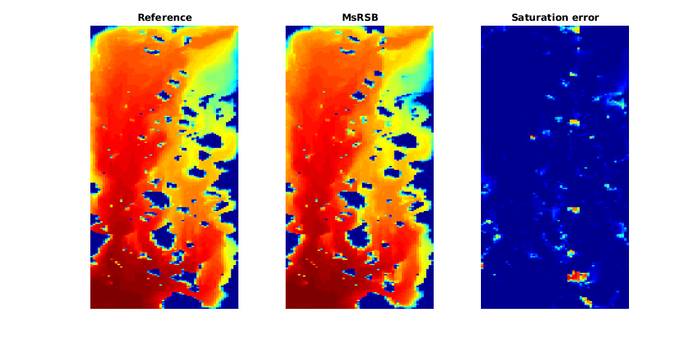
Simulate a transport problem with the MsRSB method

Generated from SPE10Layer2phMS.m

This example is a simple demonstration in how to use the multiscale solver to solve a transport problem using the incomp module.

mrstModule add mrst-gui spe10 coarsegrid incomp

Set up the fine-scale model

We set up a layer of SPE10, just as in the introductory single-phase exampleMs example.

% Grid an petrophysics
layerNo = 85;
[G, ~, rock] = getSPE10setup(layerNo);
mp = 0.01;
rock.poro(rock.poro < mp) = mp;

% Transmissibilities on fine scale
T = computeTrans(G, rock);

% Inject 1 PV over 10 years
time = 10*year;
Nt = 100;
pv = poreVolume(G, rock);

% Set up wells in each corner
injr = sum(pv)/(time);
W = [];
W = verticalWell(W, G, rock, 1, 1, [], 'type', 'rate', ...
    'val', injr, 'comp_i', [1, 0]);
W = verticalWell(W, G, rock, G.cartDims(1), G.cartDims(2), [],...
    'type', 'bhp' , 'val', 100*barsa, 'comp_i', [1, 0]);

% Plot the permeability field (log-scale).
figure(1); clf
plotToolbar(G, log10(rock.perm(:, 1)));
axis equal tight off
colormap jet
view(90, 90);

Define coarse partition and support regions

Set up a uniform coarsegrid

mrstModule add msrsb

coarsen = [5 10 5];
coarsedims = ceil(G.cartDims./coarsen);

% Generate partition vector
p = partitionUI(G, coarsedims);
% Grid structure from partition vector
CG = generateCoarseGrid(G, p);
% Add centroids / geometry information on coarse grid
CG = coarsenGeometry(CG);
% Store the support of each cell (used by multiscale basis construction)
CG = storeInteractionRegionCart(CG);

Set up basis functions

A = getIncomp1PhMatrix(G, T);
basis = getMultiscaleBasis(CG, A, 'type', 'msrsb');

Simulate the problem

We simulate the whole injection period with a fluid model with equal viscosities and quadratic Corey coefficients for the relative permeability. Since the total mobility does not change significantly, we opt to keep the basis functions static throughout the simulation. Moreover, we only use a single multiscale solve and do not introduce extra iterations to reduce the fine-scale residual towared machine precision. As a result, the multiscale approximation will deviate somewhat from the fine-scale TPFA solution.

dt = time/Nt;
figure(1);
set(gcf, 'position', [50, 50, 1000, 500])

fluid = initSimpleFluid('mu', [1, 1]*centi*poise, 'n', [2, 2], 'rho', [0, 0]);

state0 = initResSol(G, 0, [0, 1]);
gravity reset off

psolve = @(state) incompTPFA(state, G, T, fluid, 'Wells', W);
mssolve = @(state) incompMultiscale(state, CG, T, fluid, basis, 'Wells', W);
solver = @(state) implicitTransport(state, G, dt, rock, fluid, 'wells', W);

states = psolve(state0);
states_ms = mssolve(state0);

h = waitbar(0, 'Starting simulation...');
for i = 1:Nt
    waitbar(i/Nt, h, sprintf('Step %d of %d: ', i, Nt))

    state = psolve(states(end));
    states = [states; solver(state)];

    state = mssolve(states_ms(end));
    states_ms = [states_ms; solver(state)];

    s_ms = states_ms(end).s(:, 1);
    s_ref = states(end).s(:, 1);
    figure(1), clf
    subplot(1, 3, 1)
    plotCellData(G, s_ref, 'EdgeColor', 'none')
    axis tight off
    title('Reference');

    subplot(1, 3, 2)
    plotCellData(G, s_ms, 'EdgeColor', 'none')
    axis tight off
    title('MsRSB')

    subplot(1, 3, 3)
    plotCellData(G, abs(s_ref - s_ms), 'EdgeColor', 'none')
    axis tight off
    caxis([0, 1])
    title('Saturation error')
    drawnow
end
close(h)

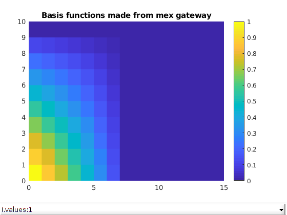
MsRSB basis function with mex acceleration

Generated from acceleratedMultiscaleBasisGenerationExample.m

The MsRSB basis functions can be efficiently computed using a compiled function written in C++. If a C++ compiler is available, this is generally an order of magnitude faster than using the Matlab version. In this example, we demonstrate the syntax for generating basis functions either directly from Matlab or via a flat file format.

mrstModule add coarsegrid msrsb libgeometry incomp
% Some different test cases
testcase = 'simple';

switch lower(testcase)
    case 'simple'
        G = cartGrid([15, 10]);
        rock = makeRock(G, 1, 1);
        p = partitionUI(G, [3, 2]);
    case 'medium'
        G = cartGrid([80, 40]);
        rock = makeRock(G, 1, 1);
        p = partitionUI(G, [8, 4]);
    case 'big'
        G = cartGrid([50, 50, 20]);
        rock = makeRock(G, 1, 1);
        p = partitionUI(G, [5, 5, 2]);
    case 'huge'
        G = cartGrid([200, 200, 100]);
        rock = makeRock(G, 1, 1);
        p = partitionUI(G, [10, 10, 10]);
        G = mcomputeGeometry(G);
    case 'spe10'
        mrstModule add spe10
        layers = 1:85;
        [G, ~, rock] = getSPE10setup(layers);
        p = partitionUI(G, [6, 11, ceil(G.cartDims(3)./5)]);
    otherwise
        error('Unknown test case %s', testcase);
end

if ~isfield(G.cells, 'centroids')
    G = computeGeometry(G);
end

T = computeTrans(G, rock);
A = getIncomp1PhMatrix(G, T);

CG = generateCoarseGrid(G, p);
CG = coarsenGeometry(CG);
CG = storeInteractionRegionCart(CG);

Add extra data to coarse grid

The function setupMexInteractionMapping adds additional mappings to the coarse grid which are required for the compiled interface. This can be done once for a specific coarse-fine grid pair and reused throughout a simulation.

CG = setupMexInteractionMapping(CG);

Generate basis functions via regular mex interface

Typical usage. We send in the coarsegrid and the mex layer passes values onto the C++ code.

I = cppMultiscaleBasis(CG, A, 'verbose', true, 'omega', 2/3,...
                              'maxiter', 250, 'tolerance', 0.001);

Recieved 9 input arguments and requested 1 outputs
Matlab matrix processed in 0 ms
Discovered problem with 150 cells and 6 blocks
Problem has 150 equations with up to 4 connections and support in 612 cells total.
Max number of threads: 8
Creating mappings...
Starting basis generation...
Starting smoothing iterations... done after 75 iterations.
...

Generate basis functions via general interface

This is also supported through the general interface for basis functions.

basis = getMultiscaleBasis(CG, A, 'useMex', true, 'type', 'msrsb');

Recieved 9 input arguments and requested 1 outputs
Matlab matrix processed in 0 ms
Discovered problem with 150 cells and 6 blocks
Problem has 150 equations with up to 4 connections and support in 612 cells total.
Max number of threads: 8
Creating mappings...
Starting basis generation...
Starting smoothing iterations... done after 50 iterations.
...

Write a testcase to flatfiles on disk

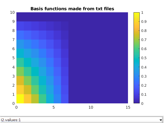
We can also write basis functions to disk as a series of text files. This is not efficient, but it is useful for setting up and running testcases without running a full Matlab session, or for generating basis functions for some other purpose.

fn = fullfile(mrstDataDirectory(), 'tmp', ['basis_', lower(testcase)]);
if ~exist(fn, 'dir')
    cppMultiscaleBasis(CG, A, 'doSolve', false, 'writePath', fn);
end

disp('Stored files:')
ls(fullfile(fn, 'input'))

Stored files:
info.txt  matrix.txt  operator.txt  sparsity.txt  support.txt  types.txt

Pass the filename to the mex function

The function will read the files and produce output in a folder named output. Once it is done, it will be read in and returned as the same type of sparse matrix.

I2 = cppMultiscaleBasisFromFile(fn);

Recieved 1 input arguments and requested 0 outputs
Matrix is 150 by 4
Creating mappings...
Starting basis generation...
Starting smoothing iterations... done after 100 iterations.
Basis generation done in 2 ms
---- Mapping generation: 0ms
---- Basis functions   : 2ms
...

Plot the basis functions

mrstModule add mrst-gui
close all;

figure;
plotToolbar(G, I);
colorbar
title('Basis functions made from mex gateway')

figure;
plotToolbar(G, I2);
colorbar
title('Basis functions made from txt files')

Multiscale solver applied to high-resolution bed model

Generated from bedModelMS.m

Pinchouts will create unstructured non-neighboring connections and hence be one of the principal gridding challenges for real-life reservoir models. To exemplify, we consider a highly detailed, core-scale model of realistic bedding structures. Such models are used as input to derive directional permeability for a given lithofacies and identify net pay below the level of petrophysical log resolution. The bedding structure consists of six different rock types and is realized on a 30x30x333 corner-point grid. Almost all cells are affected to some degree by pinch: Although the model has approximately 300.000 cells initially, over 2/3 will be inactive due to significant erosion, giving a fine grid consiting of approximately 30x30x100 cells. The volumes of the cells, as well as the areas of the (vertical) faces, vary almost four orders of magnitude. This makes the model challenging to partition. The model not only has a difficult geometry, but also has a large number of low-permeable shale layers pinched between the other high-permeable layers. Impermeable regions like this are known to pose monotonicity problems for the MsFV method. Hereine, we demonstrate various partition strategies and show that MsRSB may also suffer from severe monotonicity violations in special cases.

mrstModule add mrst-gui incomp coarsegrid msrsb
gravity off

Load model

This is one of the standard data sets that come along with MRST and can be downloaded automatically from our webpages.

pth    = getDatasetPath('bedmodel2');
grdecl = readGRDECL(fullfile(pth, 'BedModel2.grdecl'));
% pth    = getDatasetPath('bedmodels1');
% grdecl = readGRDECL(fullfile(pth,'testModel1.grdecl'));
usys   = getUnitSystem('METRIC');
grdecl = convertInputUnits(grdecl, usys);

G = processGRDECL(grdecl);
G = computeGeometry(G);

rock = grdecl2Rock(grdecl, G.cells.indexMap);

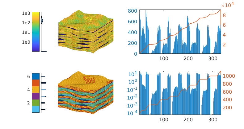
Plot the petrophysical data

The model contains rock type information in the form of the SATNUM keyword. Plot the permeability, the facies, as well as the number of cells and pore volume per layer in the grid

Kx       = convertTo(rock.perm(:,1),milli*darcy);
facies  = grdecl.SATNUM(G.cells.indexMap);
[~,~,K] = gridLogicalIndices(G);
ncell   = accumarray(K,1);
pvols   = accumarray(K,poreVolume(G,rock));
vols    = accumarray(K,G.cells.volumes);
figure('Position',[300 340 780 420]);
subplot(2,2,1,'FontSize',12)
plotCellData(G,log10(Kx),'EdgeAlpha',.1);
mrstColorbar(Kx,'west',true)
view(30,30); axis tight off;

subplot(2,2,3,'FontSize',12)
plotCellData(G,facies,'EdgeAlpha',.1);
caxis([.5 6.5]); colormap(gca,flipud(lines(6)));
mrstColorbar(facies,'west')
view(30,30); axis tight off;

subplot(2,2,2,'FontSize',12)
yyaxis left, bar(ncell), axis tight
yyaxis right, plot(cumsum(ncell),'LineWidth',1)

subplot(2,2,4,'FontSize',12)
yyaxis left, bar(pvols), set(gca,'YScale','log','YTick',10.^(-4:1))
yyaxis right, plot(cumsum(pvols),'LineWidth',1), axis tight

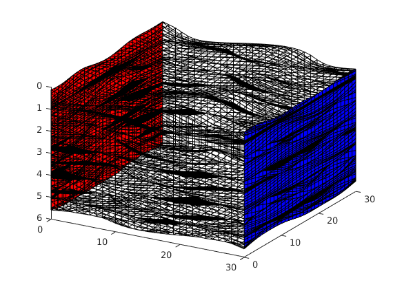
Set up and solve the fine-scale problem

Pressure drop from left to right and no-flow conditions elsewhere, single-phase fluid model with unit density and viscosity

xf    = G.faces.centroids(:, 1);
left  = find(abs(xf-min(xf))< 1e-4);
right = find(abs(xf-max(xf))< 1e-4);
bc    = addBC([], left,  'pressure', 1);
bc    = addBC(bc, right, 'pressure', 0);

figure;
plotGrid(G, 'facecolor', 'none');
plotFaces(G, left, 'facecolor', 'r')
plotFaces(G, right, 'facecolor', 'b')
view(30, 30)

fluid = initSingleFluid('rho', 1, 'mu', 1);
hT    = computeTrans(G, rock);
state = initResSol(G, 0);
ref   = incompTPFA(state, G, hT, fluid, 'bc', bc);

% Extract fine-scale matrix to use later for computing basis functions
A  = getIncomp1PhMatrix(G, hT, state, fluid);

Compute multiscale solution(s)

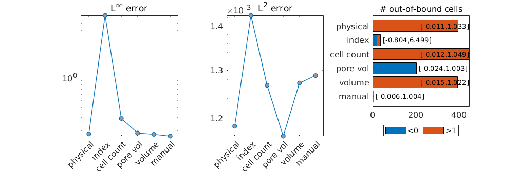
This model is challenging to partition because of the many eroded and semi-eroded layers, which we already have seen give large variations in cell sizes as well as in the number of cells and the rock volume in each layer. Many of the thin cells are strongly curved (and degenerate) so that the centroids fall outside the cell volume. Straightforward approaches, like a load-balanced partition in index space or using cell coordinates (centroids or vertices) to partition the cells into rectangular boxes in physical space can in some cases lead to grid blocks that give strong monotonicity violations. We thereofre investigate an alternative approach in which we merge layers vertically so that each of the merged layers have a certain “thickness” measured in cell count or bulk/pore volume. The bar charts to the right in the first plot indicate that the layers consist of nine natural groups we can use as a starting point. Once we have obtained a satisfactory vertical partition, we can use a “cookie cutter” approach, in index or physical space, to partition in the horizontal direction.

n = 6;
[ms,part] = deal(cell(n,1));
for i=1:n
    switch i
        case 1    % 6x6x9 in physical space
            part{i} = sampleFromBox(G,reshape(1:6*6*9,[6,6,9]));
            part{i} = processPartition(G, compressPartition(part{i}));

        case 2    % 6x6x9 in index space
            part{i} = partitionUI(G,[6 6 9]);
            part{i} = processPartition(G, compressPartition(part{i}));

        case 3    % vertical by cell count + 6x6 horizontal
            cl = discretize(cumsum(ncell),linspace(0,G.cells.num+1,10));
            [~,edges] = rlencode(cl);
            part{i}   = partitionLayers(G, [6 6], [1; cumsum(edges)+1]);

        case 4    % vertical by pore volume + 6x6 horizontal
            cl = discretize(cumsum(pvols),linspace(0,sum(pvols)*1.01,10));
            [~,edges] = rlencode(cl);
            part{i}   = partitionLayers(G, [6 6], [1; cumsum(edges)+1]);

        case 5    % vertical by bulk volume + 6x6 horizontal
            cl = discretize(cumsum(vols),linspace(0,sum(vols)*1.01,10));
            [~,edges] = rlencode(cl);
            part{i}   = partitionLayers(G, [6 6], [1; cumsum(edges)+1]);

        case 6    % custom vertical + 6x6 horizontal
            L = [1 20 58 100 145 185 220 265 305 334]';
            part{i}   = partitionLayers(G, [6 6], L);
    end
    CG = generateCoarseGrid(G, part{i});
    CG = coarsenGeometry(CG);
    CG = storeInteractionRegion(CG,'edgeBoundaryCenters', true, 'adjustCenters', true);

    % Compute basis functions
    basis = getMultiscaleBasis(CG, A, 'type', 'msrsb', 'iterations', 150);

    % Compute multiscale solution
    ms{i} = incompMultiscale(state, CG, hT, fluid, basis, 'bc', bc);
end

Handled coarse block 1 / 328
Handled coarse block 2 / 328
Handled coarse block 3 / 328
Handled coarse block 4 / 328
Handled coarse block 5 / 328
Handled coarse block 6 / 328
Handled coarse block 7 / 328
Handled coarse block 8 / 328
...

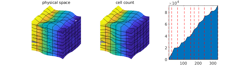
Visualize two of the solutions

figure('Position',[300 200 1000 280])
titles = {'physical space', 'index space', ...
    'cell count', 'pore volume', 'bulk volume', 'manual'};
selection = [1 3];
for i=1:2
    subplot(1,3,i)
    plotCellData(G, ms{selection(i)}.pressure, 'EdgeAlpha',.1);
    view(30,30), axis tight off
    outlineCoarseGrid(G, part{selection(i)},'FaceColor','none');
    title(titles{selection(i)},'FontWeight','normal','FontSize',12)
    caxis([-1/32 33/32]);
end
colormap([1 1 1; parula(32); .7 .7 .7]);

% show the cell count partition
subplot(1,3,3)
cl = discretize(cumsum(ncell),linspace(0,G.cells.num+1,10));
[~,edges] = rlencode(cl);
L = [1; cumsum(edges)+1];
area(cumsum(ncell));
hold on,
for i=1:numel(L)
    plot(L([i i]),[1 G.cells.num],'r--','LineWidth',1);
end
axis tight, set(gca,'FontSize',12);

Compute discrepancies and monotonicity violations

pv      = poreVolume(G,rock);
errinf  = @(x) abs(x.pressure - ref.pressure)/(max(ref.pressure) - min(ref.pressure));
err2    = @(x) sum((x.pressure - ref.pressure).^2.*pv)./sum(pv);
labels = {'physical','index','cell count','pore vol','volume','manual'};
fprintf(1,'\n%-10s%-8s\t%-8s\t%-8s\t%-8s\n','method','L2','mean','max','std');
l2err   = zeros(n,1);
linf    = zeros(n,1);
violate = zeros(n,2);
range   = zeros(n,2);
for i=1:n
    l2err(i) = err2(ms{i});
    err      = errinf(ms{i});
    linf(i)  = max(err);
    violate(i,1) = sum(ms{i}.pressure<0);
    violate(i,2) = sum(ms{i}.pressure>1);
    range(i,1)   = min(ms{i}.pressure);
    range(i,2)   = max(ms{i}.pressure);
    fprintf(1,'%-10s%.2e\t%.2e\t%.2e\t%.2e\n', labels{i},...
        err2(ms{i}), mean(err), max(err), std(err));
end
figure('Position',[300 200 1000 340])
subplot(1,3,1)
semilogy(linf,'-o','LineWidth',1,'MarkerFaceColor',[.6 .6 .6]);
set(gca,'XTick',1:n,'XTickLabel',labels,'XTickLabelRotation',45, ...
    'FontSize',12,'Xlim',[.5 n+.5]);
title('L^\infty error', 'FontWeight','normal'),

subplot(1,3,2)
semilogy(l2err,'-o','LineWidth',1,'MarkerFaceColor',[.6 .6 .6]);
set(gca,'XTick',1:n,'XTickLabel',labels,'XTickLabelRotation',45, ...
    'FontSize',12,'Xlim',[.5 n+.5]);
title('L^2 error', 'FontWeight','normal'),

subplot(1,3,3)
barh(violate,'stacked');
set(gca,'YTick',1:n,'YTickLabel',labels, 'YDir', 'reverse',...
    'FontSize',12,'Ylim',[.25 n+.75]);
legend('<0','>1','location','southoutside','orientation','horizontal');
for i=1:n
    h=text(min(sum(violate(i,:))+10,220),i,...
        sprintf('[%.3f,%.3f]',range(i,1),range(i,2)));
end
title('# out-of-bound cells', 'FontSize', 12, 'FontWeight','normal');

method    L2          mean            max             std
physical  1.18e-03    3.30e-02        1.84e-01        2.57e-02
index     1.43e-03    3.43e-02        6.32e+00        4.44e-02
cell count1.27e-03    3.40e-02        2.91e-01        2.76e-02
pore vol  1.16e-03    3.27e-02        1.88e-01        2.56e-02
volume    1.27e-03    3.37e-02        1.81e-01        2.59e-02
manual    1.29e-03    3.34e-02        1.72e-01        2.54e-02

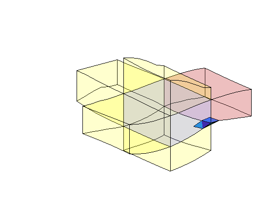
Show the worst monotonicity violation

figure
sol   = ms{2}.pressure;
p     = part{2};
ind   = unique(p(sol>1.1));
neigh = getCellNeighbors(CG,ind(1));
plotGrid(CG,ind(2),'FaceAlpha',.2,'FaceColor',[.8 .3 .3]);
plotGrid(CG,ind(1),'FaceAlpha',.1,'FaceColor',[.3 .3 .8]);
plotCellData(G,sol,sol>1.1);
plotGrid(CG,neigh,'FaceAlpha',.1);
view(3); axis tight off

Copyright notice

<html>
% <p><font size="-1

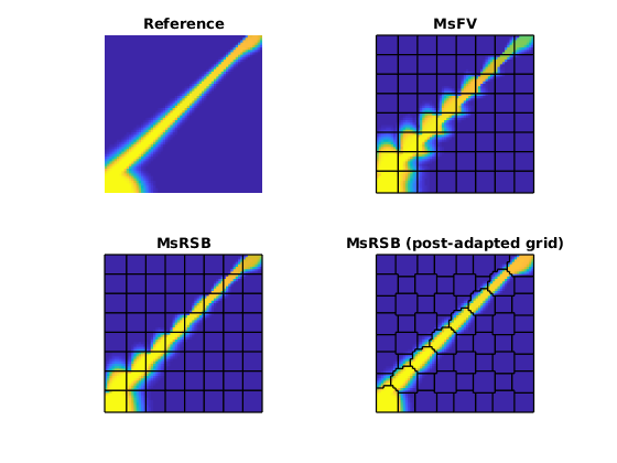
Problem comparing different multiscale methods on an idealized channel

Generated from highContrastChannelMultiscale.m

Extensive numerical experiments have shown that contemporary multiscale methods provide approximate solutions of good quality for highly heterogeneous media. However, cases with large permeability contrasts are generally challenging and it is not difficult to construct pathological test cases on which a particular method fails to produce accurate solutions. Diagonal channel. Kippe et al. proposed a simple and illuminating example consisting of a narrow high-permeable channel in a low-permeable background, where the channel is aligned with the diagonal direction. This example corresponds to Example 4.3.3 in A multiscale restriction-smoothed basis method for high contrast porous media represented on unstructured grids. J. Comput. Phys, Vol. 304, pp. 46-71, 2016. DOI: 10.1016/j.jcp.2015.10.010

% Load modules
mrstModule add msrsb incomp coarsegrid mrst-gui msfvm matlab_bgl

We set up the domain

The domain consists of 65 by 65 fine cells and a permeability field that is equal to 10 mD everywhere except for a narrow channel that crosses the domain diagonally, where the permeability is 1000 mD.

dims = [65, 65];
pdims = [1000 1000]*meter;
G = cartGrid(dims, pdims);
G = computeGeometry(G);

% Alternate intersection can be inserted. This channel crosses the blocks
% diagonally and is not a problem for either finite-volume multiscale
% scheme.
% x1 = repmat([0, 0, 0], G.cells.num, 1);
% x2 = repmat([1, 1, 0], G.cells.num, 1);
x1 = repmat([0.0, 0.05, 0], G.cells.num, 1);
x2 = repmat([0.95, 1.0, 0], G.cells.num, 1);

% Insert channel based on distance
x0 = [bsxfun(@rdivide, G.cells.centroids, pdims), zeros(G.cells.num, 1)];
dist = sqrt(sum(cross(x2 - x1, x1 - x0).^2, 2)./sum((x2 - x1).^2, 2));
isChannel = dist < 0.02;
% Set up rock structure
perm = repmat(10*milli*darcy, G.cells.num, 1);
perm(isChannel) = 1*darcy;
rock = makeRock(G, perm, 1);
% Setup unit fluid model
fluid = initSimpleFluid('rho', [1, 1], 'mu', [1, 1], 'n', [1 1]);
% Set up a coarse grid
coarsedims = [8, 8];
p = partitionUI(G, coarsedims);
% Plot the permeability field and coares grid
figure(1); clf
plotToolbar(G, rock.perm/darcy());
colorbar
axis equal tight off
outlineCoarseGrid(G, p, 'w')

Solve fine-scale problem

We simulate 1/4 pore volume injected, corresponding to the channel being completely filled. Some fluid will infiltrate into the low permeability region, which is where we will see the approximation error made by the multiscale methods clearly.

time = 1*year;
Nt = 20;
pv = poreVolume(G, rock);
% Set rate and wells in opposite corners of grid
injr = sum(pv)/(4*time);
W = [];
W = verticalWell(W, G, rock, 1, 1, [], 'type', 'rate', ...
    'val', injr, 'comp_i', [1, 0]);
W = verticalWell(W, G, rock, G.cartDims(1), G.cartDims(2), [],...
    'type', 'bhp' , 'val', 1*barsa, 'comp_i', [1, 0]);

% Solve pressure field for fine scale
state0 = initResSol(G, 0, [0, 1]);
T = computeTrans(G, rock);
ref = incompTPFA(state0, G, T, fluid, 'MatrixOutput', true, 'Wells', W);

Coarse grid and basis functions

Grid structure from partition vector

CG = generateCoarseGrid(G, p);
% Add centroids / geometry information on coarse grid
CG = coarsenGeometry(CG);
% Store the support of each cell (used by multiscale basis construction)
% Set up coarse grid
blockPts = CG.cells.centroids;
% Set the interaction/support regions to be as simple as possible for MsRSB
CG = storeInteractionRegion(CG, 'adjustCenters', false, ...
                                'localTriangulation', false, ...
                                'centerOverride', blockPts);
% Set up dual grid - required for classical MsFV-method
DG = partitionUIdual(CG, coarsedims);
DG = makeExplicitDual(CG, DG);
CG.dual = DG;

% Compute basis functions, use very strict tolerance and an excessive
% amount of iterations to avoid any round-of error from basis functions not
% being converged. For this reason, we use a C-accelerated version of the
% MsRSB solver. If this fails to compile on your computer, you can change
% the 'useMex' argument to false and wait a little longer for the result.
A = getIncomp1PhMatrix(G, T);
basisfv = getMultiscaleBasis(CG, A, 'type', 'msfvm');
msfv = incompMultiscale(state0, CG, T, fluid, basisfv, 'wells', W);
basis = getMultiscaleBasis(CG, A, 'type', 'msrsb', 'useMex', true, ...
                                  'iterations', 1000,'tolerance', 1e-4);
% Create a second coarse grid that adapts to the already computed basis
% functions (see paper for more details).
basis2 = basis;
CG2 = basisToCoarseGrid(G, basis2.B);
basis2.R = controlVolumeRestriction(CG2.partition);

ms = incompMultiscale(state0, CG, T, fluid, basis, 'wells', W);
ms2 = incompMultiscale(state0, CG2, T, fluid, basis2, 'wells', W);

Handled coarse block 1 / 64
Handled coarse block 2 / 64
Handled coarse block 3 / 64
Handled coarse block 4 / 64
Handled coarse block 5 / 64
Handled coarse block 6 / 64
Handled coarse block 7 / 64
Handled coarse block 8 / 64
...

Simulate time loop

We do not need to update the pressure for either solver, as the unit fluid results in no mobility changes during the simulation

dt = time/Nt;
tsolve = @(state) implicitTransport(state, G, dt, rock, fluid, 'wells', W);
for j = 1:Nt
    fprintf('%d of %d \n', j, Nt);

    disp('Solving MsRSB')
    ms = [ms; tsolve(ms(end))];
    disp('Solving MsRSB [a posteriori adaption]')
    ms2 = [ms2; tsolve(ms2(end))];
    disp('Solving MsFV')
    msfv = [msfv; tsolve(msfv(end))];
    disp('Solving TPFA')
    ref = [ref; tsolve(ref(end))];
end

1 of 20
Solving MsRSB
Solving MsRSB [a posteriori adaption]
Solving MsFV
Solving TPFA
2 of 20
Solving MsRSB
Solving MsRSB [a posteriori adaption]
...

Finally, plot the results

figure;
subplot(2, 2, 1)
plotCellData(G, ref(end).s(:, 1), 'EdgeColor', 'none')
axis equal tight off
caxis([0, 1])
title('Reference')

subplot(2, 2, 2)
plotCellData(G, msfv(end).s(:, 1), 'EdgeColor', 'none')
axis equal tight off
caxis([0, 1])
title('MsFV')
outlineCoarseGrid(G, CG.partition, 'w', 'linewidth', 1)

subplot(2, 2, 3)
plotCellData(G, ms(end).s(:, 1), 'EdgeColor', 'none')
axis equal tight off
caxis([0, 1])
title('MsRSB')
outlineCoarseGrid(G, CG.partition, 'w', 'linewidth', 1)

subplot(2, 2, 4)
plotCellData(G, ms2(end).s(:, 1), 'EdgeColor', 'none')
axis equal tight off
caxis([0, 1])
title('MsRSB (post-adapted grid)')
outlineCoarseGrid(G, CG2.partition, 'w', 'linewidth', 1)

Copyright notice

<html>
% <p><font size="-1

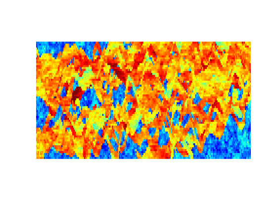
Multiscale solver with inactive cells / inclusions

Generated from inclusionsMultiscale.m

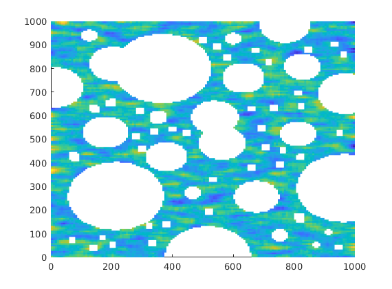
A tough test case for any multiscale solver is a grid with many inactive cells that make coarse grids highly challenging. This example demonstrates the robustness of MsRSB when faced with a large number of inactive cells. This example corresponds to Example 4.3.5 in A multiscale restriction-smoothed basis method for high contrast porous media represented on unstructured grids. J. Comput. Phys, Vol. 304, pp. 46-71, 2016. DOI: 10.1016/j.jcp.2015.10.010

mrstModule add  msrsb coarsegrid mrst-gui incomp

Grid and petrophysics

We have stored a image containing the inclusions

img = imread(fullfile(mrstPath('msrsb'), 'examples', 'inclusions.png'));
img = double(img(:,:,1));

dims = size(img);
pdims = [1 1]*kilo*meter;
G = cartGrid(dims, pdims);
active = find(img == 255);

% Extract active cells
G = extractSubgrid(G, active);
G = computeGeometry(G);

% Create a simple log-normal permeability field and map onto active subset
k = logNormLayers(G.cartDims);
perm = k(G.cells.indexMap)*darcy;
poro = 0.5;
rock = makeRock(G, perm, poro);
T = computeTrans(G, rock);

clf,
plotCellData(G,log10(rock.perm),'EdgeColor','none')

% Single-phase unit fluid model. Since we are solving a single-phase
% incompressible problem without gravity, the values here do not matter.
fluid = initSimpleFluid('rho', [1, 1], 'mu', [1, 1], 'n', [1 1]);

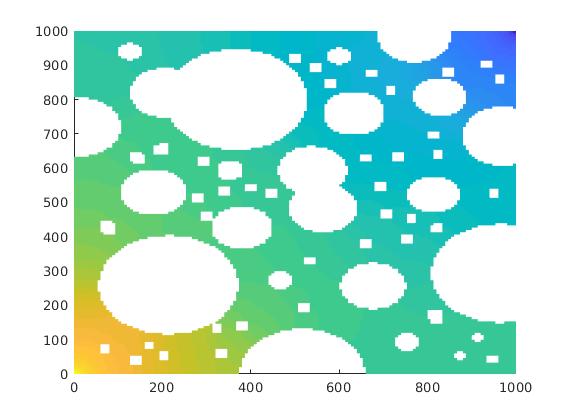
Solve fine-scale problem

We inject one pore volume over ten years with wells in opposing corners.

time = 10*year;
Nt = 100;
pv = poreVolume(G, rock);

% Set up wells in each corner
injr = sum(pv)/(time);
W = [];
W = verticalWell(W, G, rock, 1, 1, [], 'type', 'rate', ...
    'val', injr, 'comp_i', [1, 0]);
W = verticalWell(W, G, rock, G.cartDims(1), G.cartDims(2), [],...
    'type', 'bhp' , 'val', 100*barsa, 'comp_i', [1, 0]);

% Compute reference
state0 = initResSol(G, 0, [0, 1]);
ref0 = incompTPFA(state0, G, T, fluid, 'MatrixOutput', true, 'Wells', W);

clf, plotCellData(G,ref0.pressure/barsa,'EdgeColor','none');

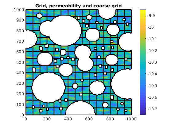
Coarse partition

simple = true;
if simple
    % Simple coarse grid
    cdims = [10, 10];
    coarsedims = ceil(G.cartDims./cdims);
    p = partitionUI(G, coarsedims);
else
    % Alternative: Use Metis (if installed)
    p = partitionMETIS(G, T, 200); %#ok<UNRCH>
end
p = processPartition(G, p);
p = compressPartition(p);

% Plot the grid, log10 of permeability and coarse grid
clf
plotCellData(G, log10(rock.perm), 'EdgeColor', 'none')
outlineCoarseGrid(G, p, 'k')
title('Grid, permeability and coarse grid')
axis equal tight
colorbar

Coarse grid and basis functions

Generate partition vector

CG = generateCoarseGrid(G, p);
% Add centroids / geometry information on coarse grid
CG = coarsenGeometry(CG);
% Store the support of each cell (used by multiscale basis construction)
CG = storeInteractionRegionCart(CG);
A = getIncomp1PhMatrix(G, T);
% Compute basis and solve for multiscale flux/pressure.
basis = getMultiscaleBasis(CG, A, 'type', 'msrsb');
ms0 = incompMultiscale(state0, CG, T, fluid, basis, 'wells', W);

Warning: Matrix is close to singular or badly scaled. Results may be inaccurate.
RCOND =  3.203665e-36.

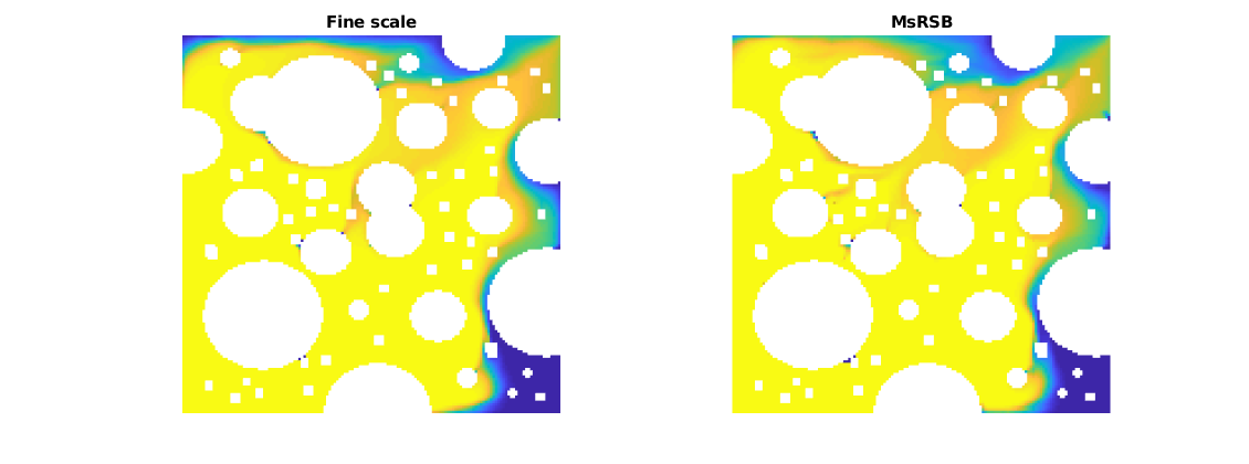
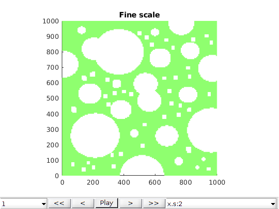
Solve the time loop, and plot saturations as they progress

dt = time/Nt;
tsolve = @(state) implicitTransport(state, G, dt, rock, fluid, 'wells', W);
ref = ref0;
ms = ms0;
figure(1);
df = get(0, 'DefaultFigurePosition');
set(gcf, 'Position', df.*[1, 1, 2, 1])
for j = 1:Nt
    fprintf('%d of %d \n', j, Nt);

    disp('Solving MsRSB')
    ms = [ms; tsolve(ms(end))];
    disp('Solving TPFA')
    ref = [ref; tsolve(ref(end))];

    figure(1); clf
    subplot(1, 2, 1)
    plotCellData(G, ref(end).s(:, 1), 'EdgeColor', 'none')
    axis equal tight off
    caxis([0, 1])
    title('Fine scale')

    subplot(1, 2, 2)
    plotCellData(G, ms(end).s(:, 1), 'EdgeColor', 'none')
    axis equal tight off
    caxis([0, 1])
    title('MsRSB')
    drawnow
end

1 of 100
Solving MsRSB
Solving TPFA
2 of 100
Solving MsRSB
Solving TPFA
3 of 100
Solving MsRSB
...

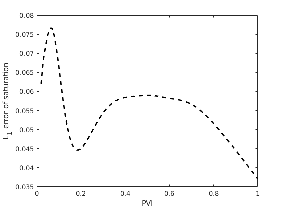
Plot L1 norm of the error in saturation

We plot the saturation error with respect to the number of pore volumes injected.

L1 = @(x, y) norm(x - y, 1)/norm(y, 1);
err = arrayfun(@(x, y) L1(x.s(:, 1), y.s(:, 1)), ms, ref);

figure;
plot((1:numel(err))./numel(err), err, 'k--', 'linewidth', 2)
xlabel('PVI')
ylabel('L_1 error of saturation')

Launch interactive plotting

plotter = @(x) plotToolbar(G, x, 'field', 's:2');
close all
cmap = jet();
h1 = figure; plotter(ref);
axis equal tight; colormap(cmap)
title('Fine scale')

c = caxis();
h2 = figure; plotter(ms);
axis equal tight; colormap(cmap)
title('MsRSB')
caxis(c);

Copyright notice

<html>
% <p><font size="-1

Introduction to the use of multiscale solvers as an iterative two-level method

Generated from introIterativeMultiscale.m

This example demonstrates the use of multiscale solvers as two-level multigrid-like methods. We demonstrate several different interfaces for iterative multiscale methods in MRST, depending on the intended usage. We recommend that you first go through the introMultiscale example before running this example, as we here do not detail the basic interfaces.

mrstModule add coarsegrid spe10 msrsb incomp ad-core

Define grid and rock

dims = [30, 110];
physDims = dims .*[20, 10]*ft;
% Create grid
G = cartGrid(dims, physDims);
G = computeGeometry(G);
n = G.cells.num;

% Take the rock structure from layer 15
rock = getSPE10rock(1:dims(1), 1:dims(2), 15);
rock.perm = rock.perm(:, 1);
rock.poro = max(rock.poro, 1e-3);
hT = computeTrans(G, rock);
% Coarsen into uniform grid
cdims = ceil(dims./[5, 10]);
p = partitionUI(G, cdims);
% Make coarse grid
CG = generateCoarseGrid(G, p);
% Add coarse geometry (centroids, normals, etc)
CG = coarsenGeometry(CG);
CG = storeInteractionRegion(CG);

Handled coarse block 1 / 66
Handled coarse block 2 / 66
Handled coarse block 3 / 66
Handled coarse block 4 / 66
Handled coarse block 5 / 66
Handled coarse block 6 / 66
Handled coarse block 7 / 66
Handled coarse block 8 / 66
...

Set up a problem with two wells

We here set up a problem where wells are the driving force. Wells are the most common driving forces for field-scale simulation, and can be challenging to resolve as they represent a highly localized source terms. Here, the wells are simple point-wells in the first and last cell of the domain, corresponding to each corner of a structured grid.

W = [];
W = addWell(W, G, rock, 1, 'type', 'bhp', 'val', 100*barsa);
W = addWell(W, G, rock, n, 'type', 'bhp', 'val', 50*barsa);
fluid = initSingleFluid('rho', 1, 'mu', 1);
state0 = initResSol(G, 0);
% Call fine-scale solver, with matrix output in state enabled
state = incompTPFA(state0, G, hT, fluid, 'MatrixOutput', true, 'W', W);

Warning: Inconsistent Number of Phases.  Using 1 Phase (=min([3, 1, 1])).

Get the linear system from the report

We perform a Schur complement to remove the well equations. We are doing this since we are going to use the low-level iterative solver interface, where it is expected that the linear system is n by n in size, where n is the number of cells in the domain.

A = state.A;
b = state.rhs;
[A, b, A_ww, A_wp, q_w] = eliminateWellEquations(A, b, n);
% To recover the extra equations, for some solution p, you can use
% p = recoverWellSolution(A_ww, A_wp, q_w, p)

Create multiscale basis

Build MsRSB basis functions

basis = getMultiscaleBasis(CG, A);

Set solver parameters

Solver handle for the coarse scale solver

coarse_solver = @(A_c, b_c) mldivide(A_c, b_c);
% Initial guess
p0 = [];
% Verbosity enabled
verb = true;
% Tolerance
tol = 1e-8;
% Set the maximum number of cycles
maxIterations = 100;

Get second-stage relaxation

We select a single cycle of ILU(0) as our second stage smoother. This routine provides us a function interface @(A, b) which itself returns a function handle. This final function handle is then an approximate inverse of A. We use this interface since it allows for a setup phase, for example to perform a partial factorization of A. ILU(0) is one such partial factorization, where an incomplete lower-upper factorization is performed, allowing L and U to not have more non-zero elements than A.

fn = getSmootherFunction('type', 'ilu0', 'iterations', 1);
% Perform ILU0 factorization (using Matlab's builtin routines)
prec = fn(A, b);
p_approx = prec(b);

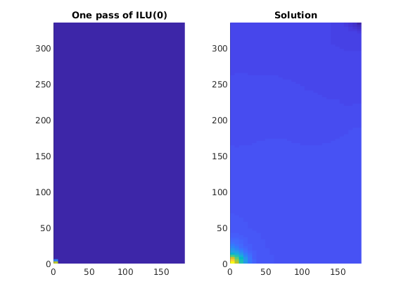
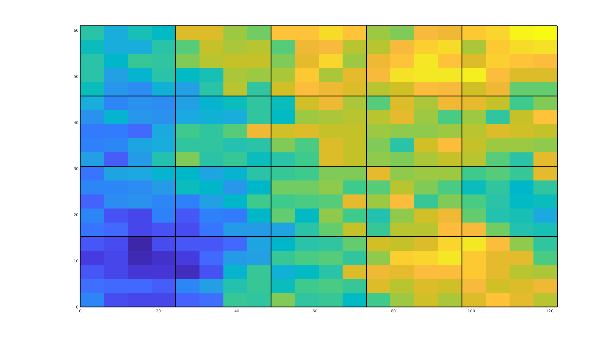
Plot the action of the preconditioner

We plot the result of a single application of ILU(0). We observe that the preconditioner only modifies the solution very close to the wells. By inheriting the sparsity pattern of the system matrix, which is a local discretization where spatial neighbors depend only on each other, a single application of the preconditioner will not account for the global nature of the elliptic pressure equation. In the parlance of multigrid and multilevel methods, ILU(0) is a smoother, as it is quite efficient at removing local (or high-frequency) errors, but not quite accurate when it comes to global (or low-frequency) errors.

clf;
subplot(1, 2, 2)
plotCellData(G, state.pressure, 'EdgeColor', 'none');
axis equal tight, cax=caxis();
title('Solution');
subplot(1, 2, 1)
plotCellData(G, p_approx, 'EdgeColor', 'none');
axis equal tight, caxis(cax);
title('One pass of ILU(0)');

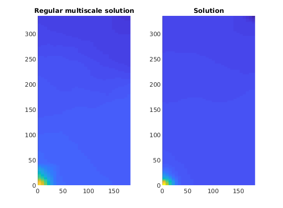
Solve and plot a regular multiscale solution

We compute a simple non-iterative multiscale approximation of the pressure field. We plot the solution together with the reference.

state_ms = incompMultiscale(state, CG, hT, fluid, basis, 'W', W);
subplot(1, 2, 1), cla
plotCellData(G, state_ms.pressure, 'EdgeColor', 'none');
axis equal tight, caxis(cax);
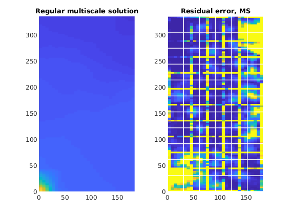
title('Regular multiscale solution');

Plot residual error in the multiscale solution

We plot the cell-wise absolute residual error,

for the multiscale solver. We observe that the error is highly localized around the support of each basis function, forming what is essentially the contours of a dual grid. This residual error is highly localized and is the result of the limited support of the basis functions, which are imposed to ensure that the coarse-scale system is sparse in nature.

subplot(1, 2, 2); cla
plotCellData(G, abs(A*state_ms.pressure - b), 'EdgeColor', 'none');
plotGrid(CG, 'EdgeColor', 'w', 'linewidth', 1, 'FaceColor', 'none')
caxis([0, 1e-10])
axis equal tight
title('Residual error, MS');

Perform two solutions: One without GMRES and one with GMRES.

The interplay between local smoothers and coarse-grid corrections is widely studied for multi-level solvers. The central idea is to use the inexpensive smoother to remove local errors, and the coarse scale solver to remove low-frequency errors. Together, the two solvers can fairly efficiently remove error modes from elliptic or near-elliptic problems. We use the low-level solveMultiscaleIteratively interface here. When useGMRES is false, a simple preconditioned Richardson iteration is performed. This problem is highly amenable to Krylov acceleration, since the error modes span multiple scales.

useGMRES = false;
[p_ms, report] = solveMultiscaleIteratively(A, b, p0, basis, fn, tol, ....
    maxIterations, coarse_solver, useGMRES, verb);
% Solve with GMRES
useGMRES = true;
[~, report_gmres] = solveMultiscaleIteratively(A, b, p0, basis, fn, tol, ...
    maxIterations, coarse_solver, useGMRES, verb);

Final residual: 8.72183e-09 after 57 iterations (tolerance: 1e-08)
Final residual: 8.9662e-09 after 17 iterations (tolerance: 1e-08)

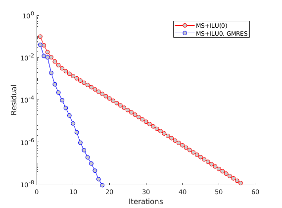
Plot the residual evolution throughout the iterative solver

We clearly observe that GMRES is much more efficient than the simple Richardson solver when measured in the number of iterations.

clf; hold on;
plot(report.resvec,'-or','MarkerFaceColor',[.8 .8 .8]);
plot(report_gmres.resvec,'-ob','MarkerFaceColor',[.8 .8 .8]);
set(gca, 'YScale', 'log')
legend('MS+ILU(0)', 'MS+ILU0, GMRES');
xlabel('Iterations');
ylabel('Residual')

We can also achieve the same result through the incompMultiscale interface

This is the easiest way of improving a multiscale solution. Here, we solve only five iterations in order to inexpensively improve upon the initial approximation.

state_ms_it = incompMultiscale(state, CG, hT, fluid, basis, 'W', W, ...
    'getSmoother', fn, 'iterations', 5, 'useGMRES', true, 'tolerance', tol);

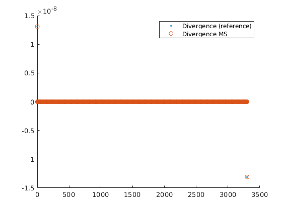
Plot discrete divergence of iterated solution

The goal of iterative multiscale methods is not necessarily to solve the solution to a very strict tolerance, but rather to get an acceptable pressure solution together with a divergence-free velocity field. Here, we plot the divergence of both the fine-scale and the iterated multiscale solutions to see that both are non-zero only in the well cells, even when the solution is not fully converged.

op = setupOperatorsTPFA(G, rock);

Div = @(flux) op.Div(flux(op.internalConn));
df = Div(state.flux);
dms = Div(state_ms_it.flux);

clf; hold on
plot(df, '.');
plot(dms, 'o');
legend('Divergence (reference)', 'Divergence MS')

Use the class-based linear solver

There is also a multiscale linear solver class for use with the ad-core framework, which uses the same internal interface.

mrstModule add ad-core
solver = MultiscaleVolumeSolverAD(CG, 'getSmoother', fn, ...
                                      'maxIterations', maxIterations,...
                                      'tolerance', tol, ...
                                      'useGMRES', true);

Solve a system

We solve a linear system with the solveLinearSystem interface. Note that this generates a basis from A, which can then be reused for subsequent solves.

sol = solver.solveLinearSystem(A, b);
disp(solver.basis)

Recieved 9 input arguments and requested 1 outputs
Matlab matrix processed in 0 ms
Discovered problem with 3300 cells and 66 blocks
Problem has 3300 equations with up to 4 connections and support in 14456 cells total.
Max number of threads: 8
Creating mappings...
Starting basis generation...
Starting smoothing iterations... done after 75 iterations.
...

Introduction to multiscale finite-volume methods

Generated from introMultiscale.m

This example introduces you to the basic concepts of multiscale finite-volume methods. To this end, we consider a single-phase flow problem written in terms of conservation of mass and Darcy’s law

Alternatively, we could write this as a variable-coefficient Poisson equation,nabla(Knabla p)=q, which is one of the primary examples of a second-order elliptic partial differential equation. The multiscale behavior of this problem comes from the coefficient K, which represents permeability and usually has large local changes and spatial correlation structures that span a wide variety of scales. To discretize the problem, we use a standard finite-volume method with a two-point flux approximation. In a standard upscaling method, one first constructs a coarse grid and then computes effective permeability values that attempt to represent the flow equation in an averaged sense on this grid. With this, one can solve the flow problem approximately using fewer unknowns. In a multiscale method, one also tries to solve the flow problem using fewer unknowns, but instead of using effective coarse-scale permeabilities, we define a set of multiscale basis functions that represent how the pressure will distribute itself locally, given a unit pressure drop between the center of one coarse grid block and the centers of all the surrounding grid blocks. Using these basis functions, we can reduce the fine-scale discretization matrix to a much smaller matrix and solve this to construct an approximate solution on the coarse grid as well as on the fine grid. We can also reconstruct mass-conservative fluxes on the fine grid or on any partition thereof. The example compares three different approximate solutions to the flow problem just described:

% This example uses several different modules.
mrstModule add coarsegrid spe10 msrsb incomp upscaling ad-core streamlines

Define grid and rock

As an example of a strongly heterogeneous problem, we consider permeability sampled from Model 2 of the SPE10 upscaling benchmark. We pick a small subset, since we are interested in examining the fine-scale linear system, which quickly becomes large as more cells are included.

dims = [20, 20];
physDims = dims .*[20, 10]*ft;
% Create grid
G = cartGrid(dims, physDims);
G = computeGeometry(G);
% Take the rock structure from layer 15
rock = getSPE10rock(1:dims(1), 1:dims(2), 15);
rock.perm = rock.perm(:, 1);
hT = computeTrans(G, rock);
% Coarsen into blocks made up of 5 x 4 fine cells
cdims = [5, 4];
p = partitionUI(G, cdims);
% Alternatively, we could make an unstructured coarse grid using, e.g., Metis
% p = partitionMETIS(G, hT, 20);

% Make coarse grid
CG = generateCoarseGrid(G, p);
% Add coarse geometry (centroids, normals, etc)
CG = coarsenGeometry(CG);

% Plot the permeability and coarse grid
figure('units', 'normalized', 'position', [0.1, .1, .8, 0.8]);
plotCellData(G, log10(rock.perm(:, 1)), 'edgec', 'none')
axis tight
plotGrid(CG,'FaceColor','none','LineWidth',2);

Define and solve the fine-scale flow problem

Set up a pressure drop along the x-axis.

bc = pside([], G, 'West', 100*barsa);
bc = pside(bc, G, 'East',  50*barsa);
fluid = initSingleFluid('rho', 1, 'mu', 1);
state0 = initResSol(G, 0);
% Call solver, with matrix output in state enabled
state = incompTPFA(state0, G, hT, fluid, 'MatrixOutput', true, 'bc', bc);
n = G.cells.num;

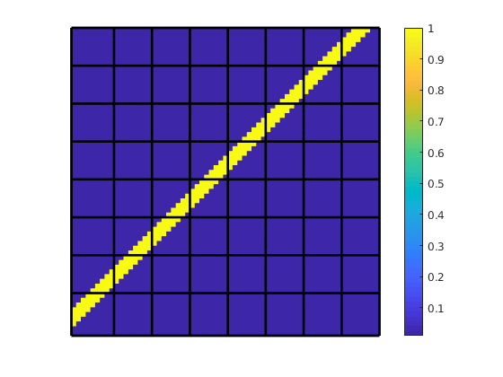
Show the fine-scale discretization

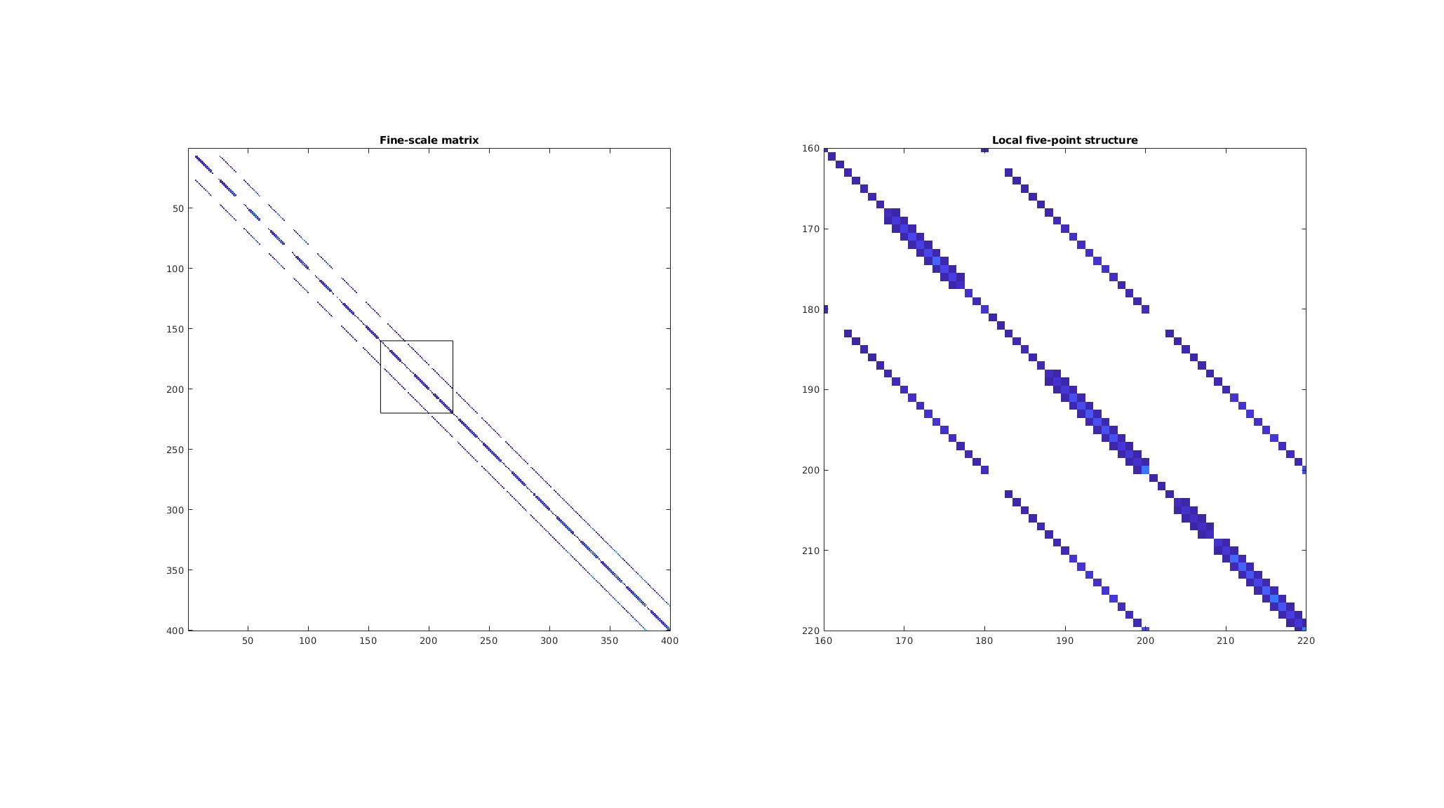
We plot the system matrix for the fine-scale system. We used a two-point flux approximation (TPFA) to solve the problem, and consequently the matrix has a banded structure for this structured grid. As each cell in a Cartesian grid has four neighbors, we get four off-diagonals bands plus the main diagonal. The incompressible pressure equation is linear, and we can thus fully translate the governing equations into the form

To show this, we plot both the full system matrix and a zoomed-in view around the degrees of freedom corresponding to a cell in the middle of the domain.

drawSquare = @(x, y) patch(x([1, 1, 2, 2]), y([1, 2, 2, 1]), 0, ...
                            'EdgeColor', 'k', 'FaceColor', 'none');
% Get system matrix from state
A = full(abs(state.A));

dx = 1.5*dims(1);
dy = 1.5*dims(2);
% We inspect a cell in the middle of the domain
inspect = sub2ind(dims, ceil(dims(1)/2), ceil(dims(2)/2));
x = [inspect - dx, inspect + dx];
y = [inspect - dy, inspect + dy];
% Plot A
clf;
subplot(1, 2, 1)
imagesc(A);
colormap([1 1 1; parula(255)]);
axis([.5 n+.5 .5 n+.5]); axis square;
hold on;
drawSquare(x, y);
title('Fine-scale matrix')
% Plot zoomed view
subplot(1, 2, 2);
imagesc(A);
ylim(x);
xlim(y);
axis square
colormap([1 1 1; parula(255)]);
title('Local five-point structure');

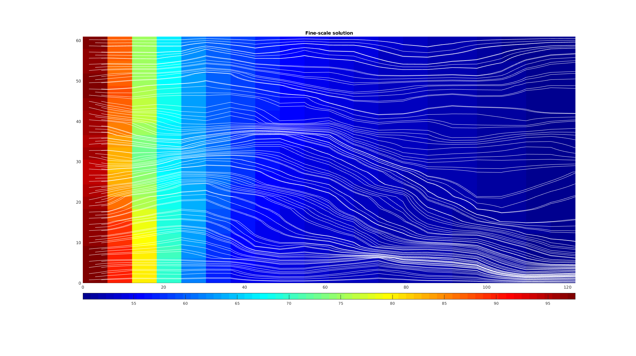
Plot the fine-scale solution together with streamlines

We plot the pressure field and trace five streamlines from each of the cells on the left boundary. Heterogeneities in the permeability field and variation in the underlying porosity result in deviation from linear flow, even with a linear pressure drop over the domain.

ijk = gridLogicalIndices(G);
cells = find(ijk{1} == 1);
p = repmat([0.25, 0.25; ...
            0.75, 0.25; ...
            0.25, 0.75; ...
            0.75, 0.75; ...
            0.5, 0.5], numel(cells), 1);
cno = rldecode(cells, 5);
startpos = [cno, p];

trace = @(state) pollock(G, state, startpos, 'pvol', rock.poro);

clf;
colormap default
plotCellData(G, state.pressure/barsa, 'edgec','none');
h = streamline(trace(state));
set(h, 'Color', 'w');
colormap(jet);
axis equal tight
title('Fine-scale solution');
colorbar('horiz')

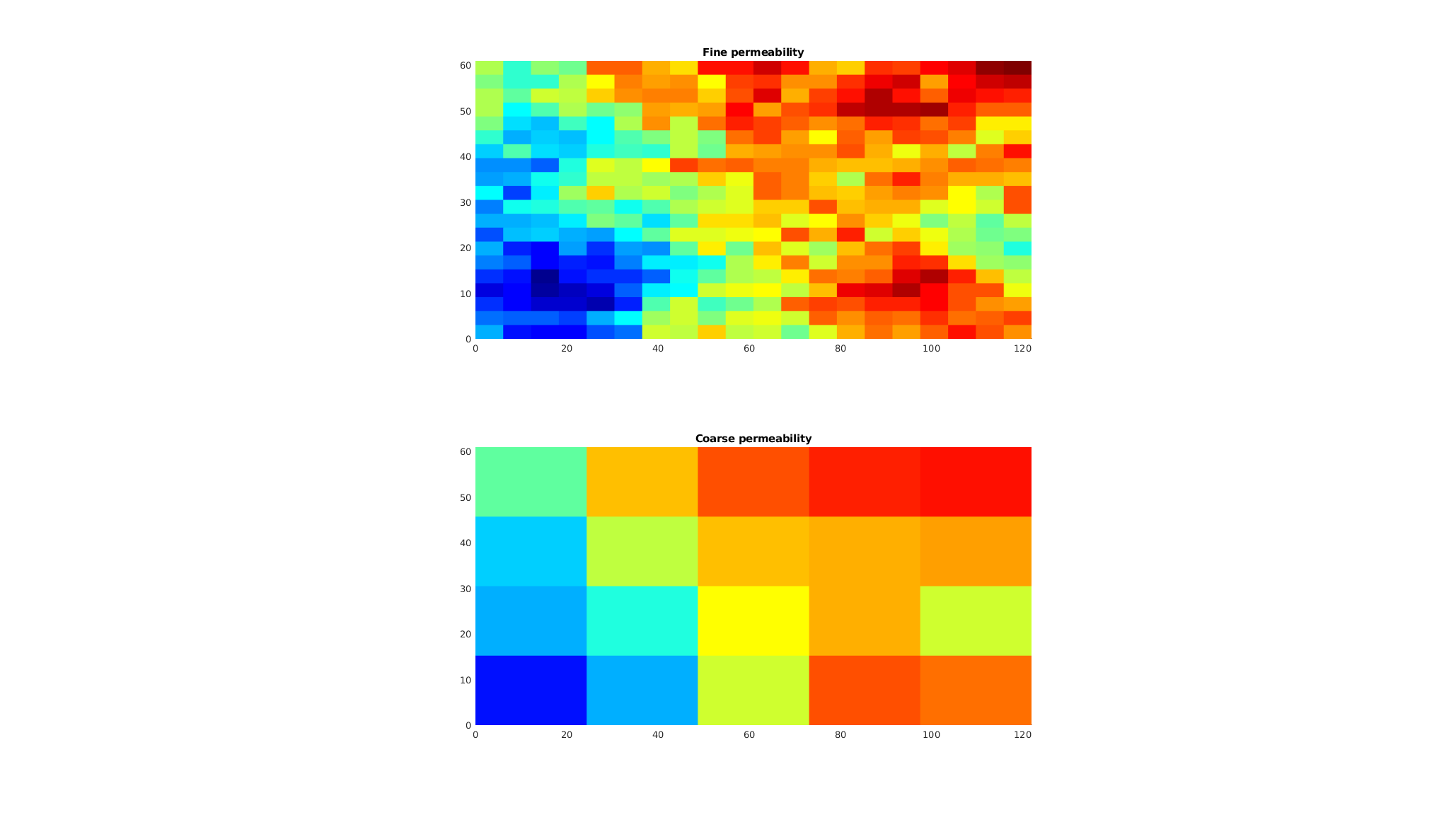
Perform upscaling of the permeability field

We create an upscaled permeability field with a flow-based upscaler from the ‘upscale’ module. In this routine, a series of local flow problem are used to get an effective coarse-scale permeability.

clf;
crock.perm = upscalePerm(G, CG, rock);

subplot(2, 1, 1);
Kf = log10(rock.perm(:,1));
plotCellData(G, Kf, 'edgec', 'none')
axis equal tight
c = caxis();
title('Fine permeability')

subplot(2, 1, 2);
Kc = log10(crock.perm(:,1));
plotCellData(CG, Kc, 'edgec', 'none')
axis equal tight
caxis(c);
title('Coarse permeability')

Solve the coarse problem

The coarse problem consists of the same governing equation as the fine-scale problem, but with an upscaled permeability field

, and posed on the coarser mesh,

With a linear system

chT = computeTrans(CG, crock);
cbc = coarsenBC(CG, bc);
cstate = initResSol(CG, 0);
cstate = incompTPFA(cstate, CG, chT, fluid, 'MatrixOutput', true, 'bc', cbc);

Solve with a multiscale solver

We now solve the problem with a multiscale solver. We do this by first generating a set of basis functions

from the system matrix. We can then form and solve a reduced problem to get the coarse multiscale pressure solution,

where

is the restriction operator and

is a matrix representation of the basis functions. For a problem with

fine cells, giving an

fine-scale system, and a coarse grid with

blocks, the basis functions and restriction operators take the form of rectangular matrices,

Due to the interpretation of the basis functions as interpolators from unit values, each entry of

takes values in

. The restriction operator can be defined in two different ways. First of all, we could set R as the transpose of P, which would give us a Galerkin formulation. Herein, we will instead use a finite-volume restriction that simply sums the rows corresponding to all cells that make up each coarse block. Thus R takes values in {0,1}.

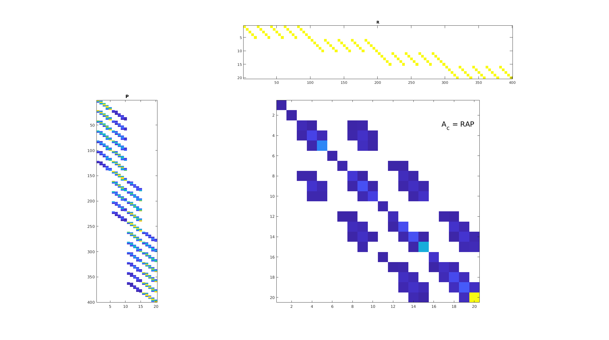
We next generate basis functions, create a coarse system, and visualize it. Since the problem is very small, we can easily visualize the systems used to construct the coarse approximation. Note that we normally use functions such as ‘incompMultiscale’ to form this coarse system, but here we explicitly write out the expressions for pedagogical reasons.

basis = getMultiscaleBasis(CG, A);
Am = basis.R*state.A*basis.B;
bm = basis.R*state.rhs;
p_ms = Am\bm;
m = CG.cells.num;
clf;
subplot(4, 4, [5, 9, 13])

imagesc(full(basis.B));
colormap([1 1 1; parula(128)]);
daspect([1, 6, 1])
axis tight
title('P');

subplot(4, 4, 2:4);
imagesc(full(basis.R));
daspect([4, 1, 1]);
axis tight
title('R')

subplot(4, 4, [6:8, 10:12, 14:16]);
imagesc(full(abs(Am))); colormap([1 1 1; parula(255)]);
axis equal tight
th = text(dims(1), 3, 'A_c = RAP', 'FontSize', 18, 'HorizontalAlignment', 'right');

Handled coarse block 1 / 20
Handled coarse block 2 / 20
Handled coarse block 3 / 20
Handled coarse block 4 / 20
Handled coarse block 5 / 20
Handled coarse block 6 / 20
Handled coarse block 7 / 20
Handled coarse block 8 / 20
...

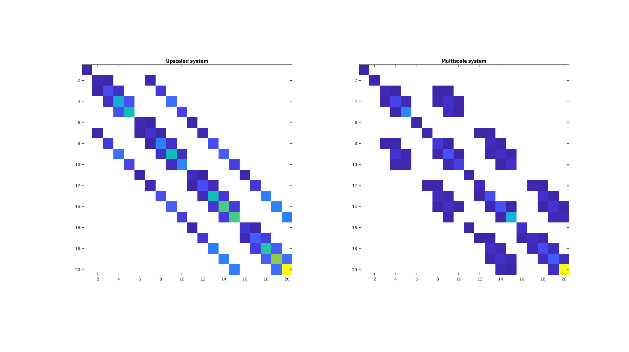
Compare the upscaled and multiscale coarse systems

Fundamentally, these two approaches are similar in that they, from fine-scale information, produce coarse-scale discretizations that seek to account for the known fine-scale structure. We observe that the upscaled system has five major diagonals, just like the original system, whereas the multiscale solver has a more irregular pattern similar to what we would get if we discretized the coarse system with a multipoint scheme. As the system is formed numerically, all nine diagonals are not fully filled in, since the magnitude of the entries depend on the basis functions.

clf;
subplot(1, 2, 1);
imagesc(full(abs(cstate.A))); colormap([1 1 1; parula(255)]);
axis equal tight
title('Upscaled system');

subplot(1, 2, 2);
imagesc(full(abs(Am))); colormap([1 1 1; parula(255)]);
axis equal tight
title('Multiscale system');

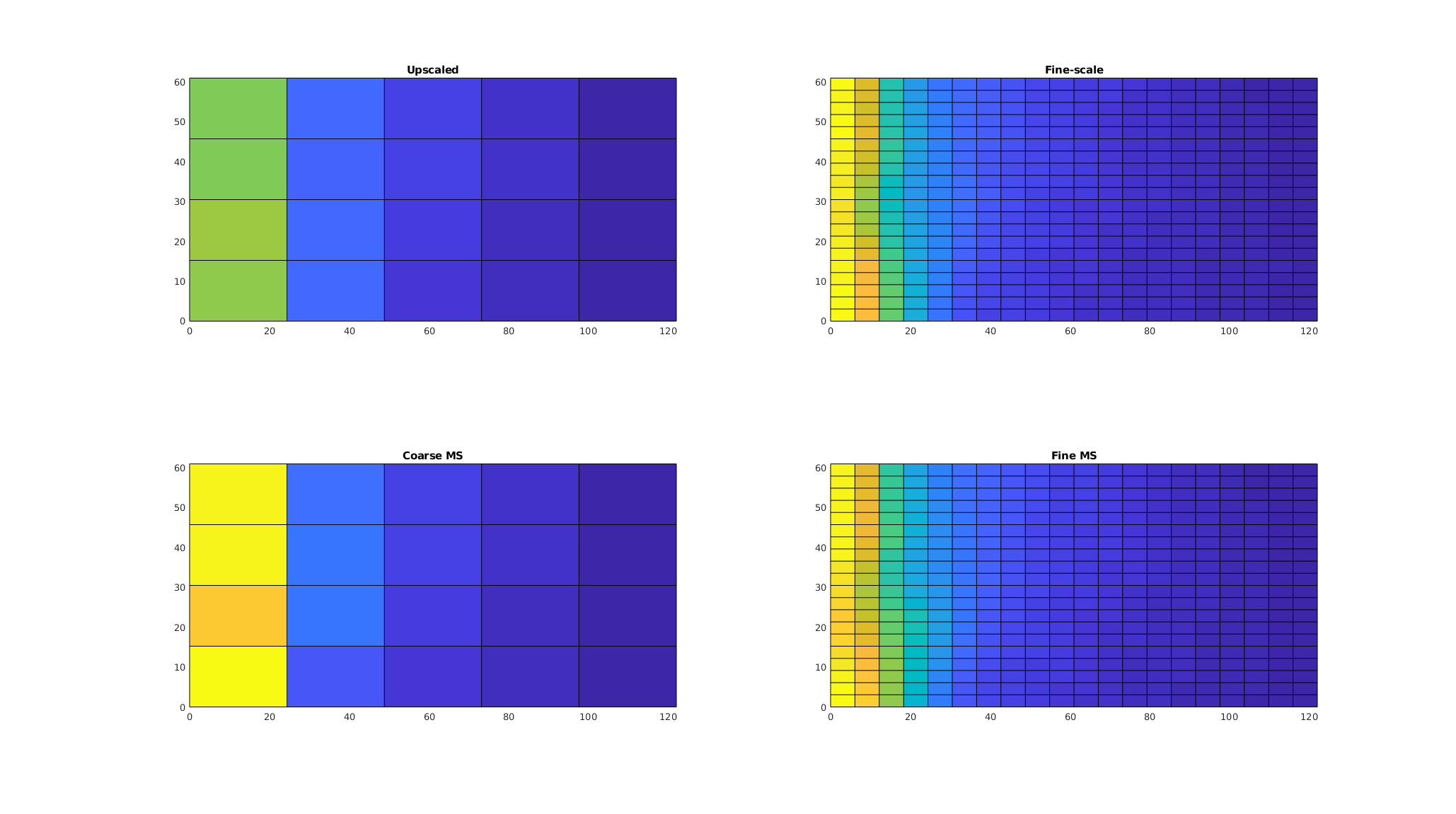
Plot the solutions

A key feature of multiscale methods is that we can create a fine-scale approximate pressure from the coarse system by applying the prolongation operator,

We plot the fine-scale reference, the two coarse-scale approximations, and the fine-scale approximation from the multiscale solver. We enforce the same color axis for all subplots, as the coarse solvers generally do not have the outliers present in the fine-scale solution.

p_upscaled = cstate.pressure;
p_fine = state.pressure;
p_prolongated = basis.B*p_ms;
ca = [min(p_fine), max(p_fine)]/barsa;

clf;
colormap default
subplot(2, 2, 1);
plotCellData(CG, p_upscaled/barsa,'EdgeColor','none');
plotFaces(CG,1:CG.faces.num)
axis equal tight;
caxis(ca);
title('Upscaled')

subplot(2, 2, 2);
plotCellData(G, p_fine/barsa);
axis equal tight;
caxis(ca);
title('Fine-scale')

subplot(2, 2, 3);
plotCellData(CG, p_ms/barsa,'EdgeColor','none');
plotFaces(CG,1:CG.faces.num)
axis equal tight;
caxis(ca);
title('Coarse MS');

subplot(2, 2, 4);
plotCellData(G, p_prolongated/barsa);
axis equal tight;
caxis(ca);
title('Fine MS');

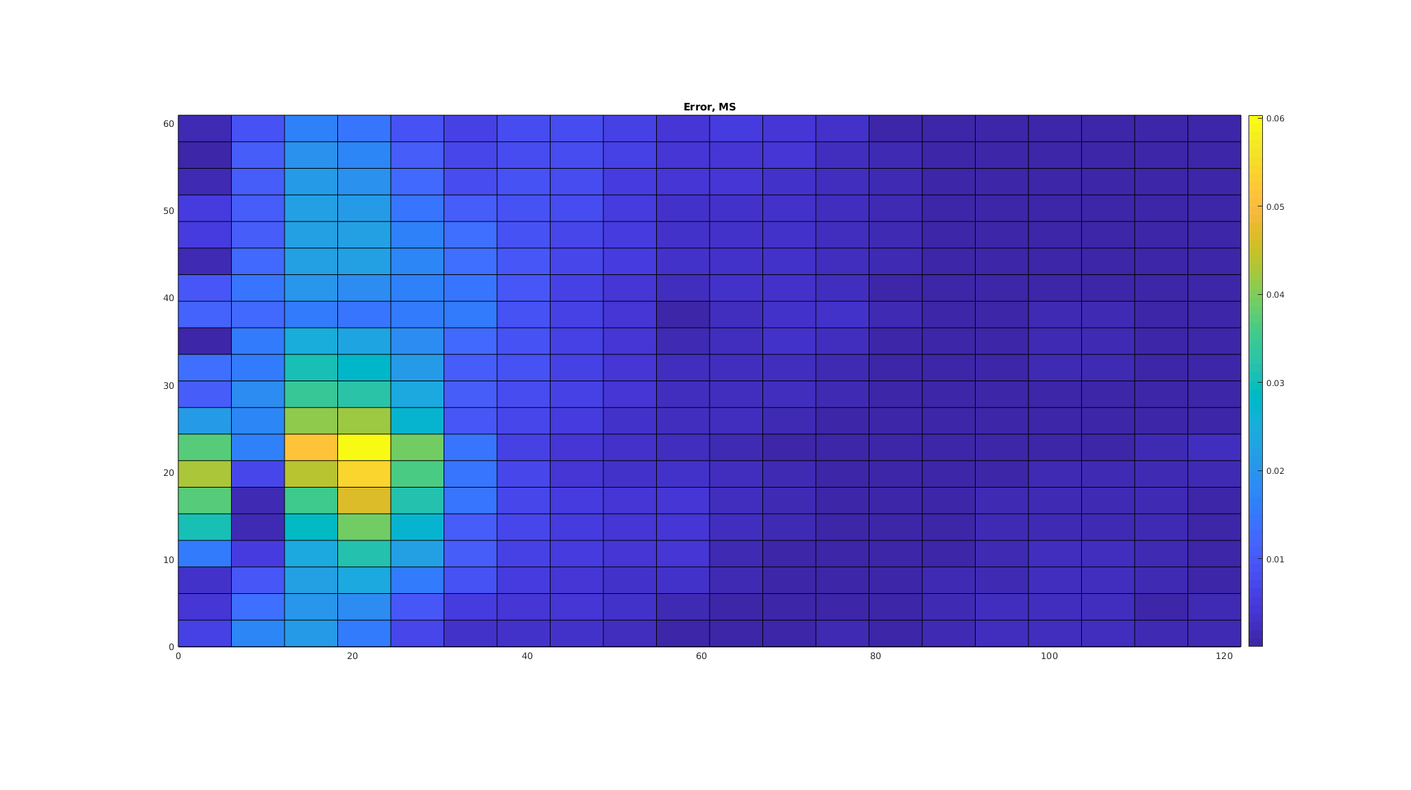
Plot the error in the fine-scale multiscale solution

The multiscale solution has two sources of error: The approximations made to ensure that the basis functions have local support, and the error in the coarse-scale system. In this case, however, the error is fairly low. We plot the scaled point-wise error

clf;
plotCellData(G, abs(p_prolongated - p_fine)/max(p_fine));
axis equal tight;
caxis auto;
colorbar
title('Error, MS');

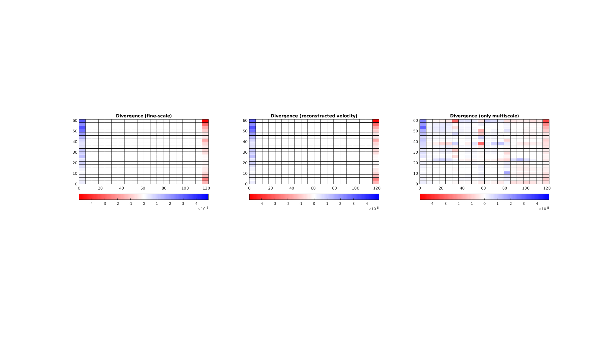
Reconstructed velocity field

A fine-scale pressure approximation is usually not our primary interest when studying a multiphase flow problem. Instead, we are typically interested in the solution of a transport equation, $$ frac{S phi}{ Delta t} + Nabla cdot (f(S) vec{v}) = q Under the limiting assumptions of incompressible, immiscible flow, we require a divergence free velocity field outside of source cells to solve this equation. The ‘incompMultiscale’ solver performs a flux reconstruction in order to produce a velocity field suitable for transport. We use the discrete divergence operator from ‘ad-core’ to verify this. If we plot the fine-scale divergence, we observe that the values are only nonzero near the boundary, where source terms are present. The same is the case for the multiscale solver when reconstruction is used, but it is not the case when we disable the flux reconstruction.

op = setupOperatorsTPFA(G, rock);

Div = @(flux) op.Div(flux(op.internalConn));
state_ms = incompMultiscale(state0, CG, hT, fluid, basis, 'bc', bc, 'reconstruct', true);
state_ms2 = incompMultiscale(state0, CG, hT, fluid, basis, 'bc', bc, 'reconstruct', false);

df = Div(state.flux);
dms = Div(state_ms.flux);
dms2 = Div(state_ms2.flux);

mv = max(max(abs(df)), max(abs(dms)));
ca = [-mv, mv];

cmap = interp1([0; 0.5; 1], [1, 0, 0; 1, 1, 1; 0, 0, 1], 0:0.01:1);

clf;
subplot(1, 3, 1)
plotCellData(G, dms);
colormap(cmap);
caxis(ca);
axis equal tight
colorbar('horiz')
title('Divergence (fine-scale)');

subplot(1, 3, 2);
plotCellData(G, dms);
colormap(cmap);
caxis(ca);
axis equal tight
colorbar('horiz')
title('Divergence (reconstructed velocity)')

subplot(1, 3, 3);
plotCellData(G, dms2);
colormap(cmap);
caxis(ca);
axis equal tight
colorbar('horiz')
title('Divergence (only multiscale)')

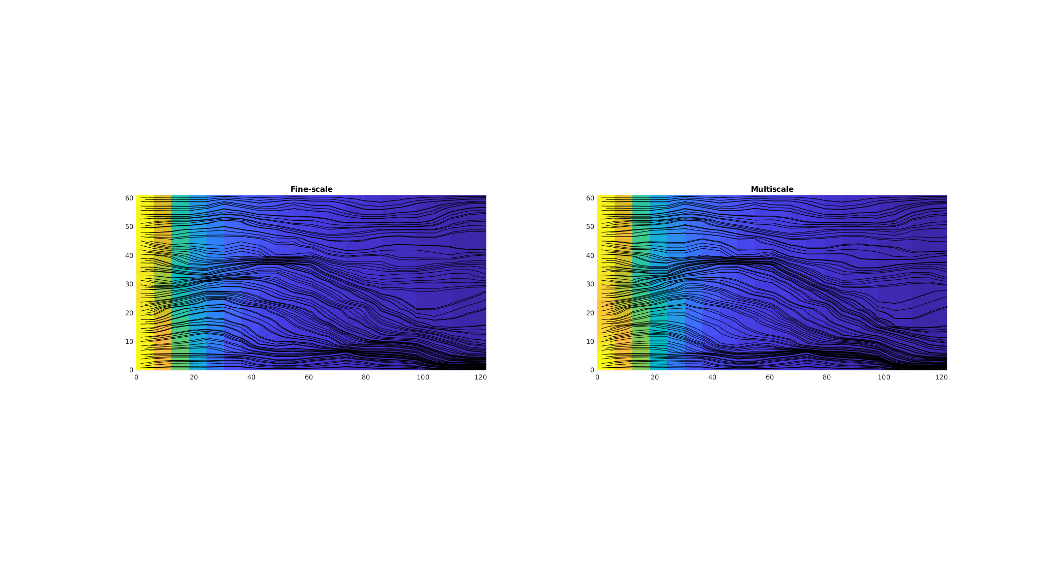
Plot fine-scale pressures side by side - together with streamlines

We have excellent agreement between the fine-scale pressures and the velocity field when visualized as streamlines.

clf
colormap default
subplot(1, 2, 1);
plotCellData(G, p_fine,'EdgeColor','none');
axis equal tight;
h = streamline(trace(state));
set(h, 'Color', 'k','linewidth',.5);
title('Fine-scale');

subplot(1, 2, 2);
plotCellData(G, p_prolongated,'EdgeColor','none');
axis equal tight;
h = streamline(trace(state_ms));
set(h, 'Color', 'k','linewidth',.5);
title('Multiscale');

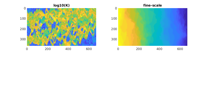
Lack of Monotonicity (Layers of SPE10)

Generated from lackOfMonotonicity.m

This example uses a single layer from the SPE10 benchmark to illustrate that multiscale solutions can give nonmonotone solutions.

mrstModule add spe10 coarsegrid incomp

Set up and solve the fine-scale model

We a single-phase fluid with unit viscosity and impose a unit pressure drop in the y-direction.

[G, ~, rock] = getSPE10setup(85);
hT    = computeTrans(G, rock);
bc    = pside([], G, 'ymin', 1);
bc    = pside(bc, G, 'ymax', 0);
fluid = initSingleFluid('rho', 1, 'mu', 1);
state = initResSol(G, 0);

figure('Position',[300 340 780 420]);
subplot(2,2,1);
plotCellData(G, log10(rock.perm(:, 1)),'EdgeColor','none');
view(90,90), axis equal tight, title('log10(K)');

subplot(2,2,2)
state = incompTPFA(state, G, hT, fluid, 'bc', bc);
plotCellData(G, state.pressure,'EdgeColor','none');
view(90,90), axis equal tight, title('fine-scale')
colormap([1 1 1; parula(32); .7 .7 .7]);
caxis([-1/32 33/32]);
% Here, we have manipulated the colorbar and caxis so that any values out
% of the pressure range described by the boundary conditions will show up
% as white for negative values and gray for values exceeding unity.

Set up coarse grid

mrstModule add msrsb
cdims = ceil(G.cartDims./[5 10 5]);
p     = partitionUI(G, cdims);
CG    = generateCoarseGrid(G, p);
CG    = coarsenGeometry(CG);
CG    = storeInteractionRegionCart(CG);

Create dual grid and add to the coarse grid

mrstModule add msfvm matlab_bgl
DG = partitionUIdual(CG, cdims);
DG = makeExplicitDual(CG, DG);
CG.dual = DG;

Processing block 1 of 299...
Processing block 2 of 299...
Processing block 3 of 299...
Processing block 4 of 299...
Processing block 5 of 299...
Processing block 6 of 299...
Processing block 7 of 299...
Processing block 8 of 299...
...

Compute basis functions

A        = getIncomp1PhMatrix(G, hT);
basis_sb = getMultiscaleBasis(CG, A, 'type', 'msrsb');
basis_fv = getMultiscaleBasis(CG, A, 'type', 'msfv');
bases    = {basis_sb, basis_fv};

Solving basis for block 1 of 299
Solving basis for block 2 of 299
Solving basis for block 3 of 299
Solving basis for block 4 of 299
Solving basis for block 5 of 299
Solving basis for block 6 of 299
Solving basis for block 7 of 299
Solving basis for block 8 of 299
...

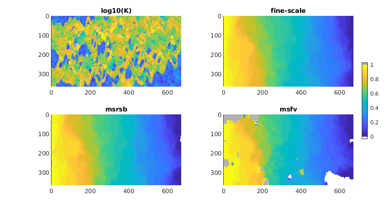
Compute multiscale solutions

Compute the MsRSB and MsFV solutions. Both schemes give multipoint stencils that lead to solutions containing values that are out of bounds, but whereas these values are barely noticable near the inflow/outflow boundaries for MsRSB, they are clearly evident in relatively large patches inside the domain for MsFV.

nb = numel(bases);
[states, reports] = deal(cell(nb, 1));
for i = 1:nb
    basis = bases{i};
    states{i} = incompMultiscale(state, CG, hT, fluid, basis, 'bc', bc);
    subplot(2,2,i+2)
    plotCellData(G, states{i}.pressure,'EdgeColor','none')
    caxis([min(state.pressure), max(state.pressure)])
    view(90,90), axis equal tight, caxis([-1/32 33/32]);
    title(bases{i}.type)
end
set(colorbar,'Position',[.925 .33 .015 .37]);

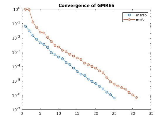
Solve using MS-GMRES

As a result of the large patches with out-of-bound values, the MsFV method has a much higher initial residual and also converges slightly slower than the MsRSB method.

fn = getSmootherFunction('type', 'ilu');
for i = 1:nb
    basis = bases{i};
    [~, reports{i}] = incompMultiscale(state, CG, hT, fluid, basis, 'bc', bc,...
        'getSmoother', fn, 'iterations', 100, 'useGMRES', true);
end
figure;
tmp = cellfun(@(x) x.resvec, reports, 'uniformoutput', false);
tmp = [tmp{:}];
if size(tmp, 1) == 1
    tmp = [tmp; tmp];
end
names = cellfun(@(x) x.type, bases, 'uniformoutput', false);
semilogy(tmp, 'o-','MarkerFaceColor',[.8 .8 .8])
legend(names)
title('Convergence of GMRES')

Copyright notice

<html>
% <p><font size="-1

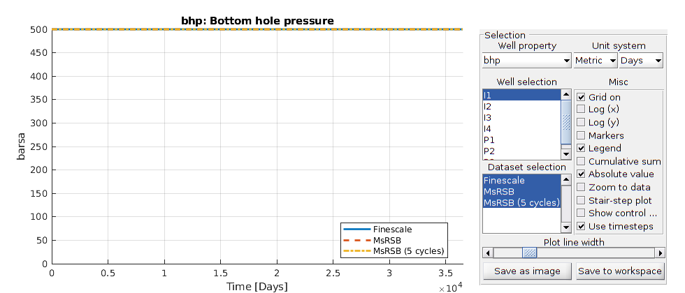
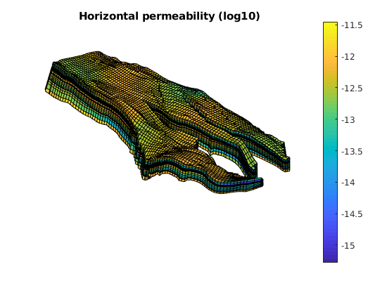
Water injection in a field model using the MsRSB-method

Generated from runNorne2phMS.m

This example demonstrates the use of the MsRSB method to a synthethic waterflood on the grid and petrophysical properties from a real field. This example is a modified version of Example 4.3.6 in A multiscale restriction-smoothed basis method for high contrast porous media represented on unstructured grids. J. Comput. Phys, Vol. 304, pp. 46-71, 2016. DOI: 10.1016/j.jcp.2015.10.010 Note that this example uses MEX-accelerated computation of basis functions which requires that MEX is set up and configured to work with an installed C++ compiler on your machine.

mrstModule add coarsegrid msrsb ad-core mrst-gui incomp

Read and set up the Norne model

We use a subset of the Norne model that is used in other examples in MRST. We set up a model with anisotropic permeability based on the vertical permeability.

mrstModule add deckformat

if ~(makeNorneSubsetAvailable() && makeNorneGRDECL())
   error('Unable to obtain simulation model subset');
end

grdecl = fullfile(getDatasetPath('norne'), 'NORNE.GRDECL');
grdecl = readGRDECL(grdecl);
usys   = getUnitSystem('METRIC');
grdecl = convertInputUnits(grdecl, usys);

G = processGRDECL(grdecl);
G = computeGeometry(G(1));
rock = grdecl2Rock(grdecl, G.cells.indexMap);

% Backwards compatible plotting
if isnumeric(gcf)
    myZoom = @zoom;
else
    myZoom = @(varargin) [];
end

Plot permeability and porosity

figure;
plotCellData(G, log10(rock.perm(:, 1)));
axis equal tight off
daspect([1 1 0.2])
view(85, 45); myZoom(1.2);
colorbar
title('Horizontal permeability (log10)')

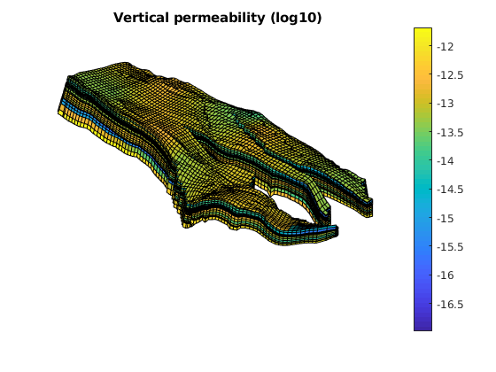
figure;
plotCellData(G, log10(rock.perm(:, 3)));
axis equal tight off
daspect([1 1 0.2])
view(85, 45); myZoom(1.2);
colorbar
title('Vertical permeability (log10)')


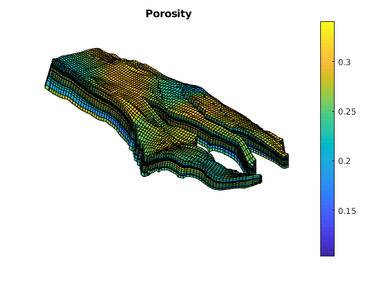
figure;
plotCellData(G, rock.poro);
axis equal tight off
daspect([1 1 0.2])
view(85, 45); myZoom(1.2);
colorbar
title('Porosity')

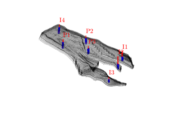
Set up wells

We set up a number of somewhat arbitrary wells around the domain. We drain a complete pore volume using three producers, with four injectors at fixed bottom hole pressures that give pressure support.

totTime = 100*year;
N_step = 100;
dt = totTime/N_step;

pv = poreVolume(G, rock);

wells = [13, 88,  -1; ...
         18, 87,  -1; ...
         36, 90,  -1; ...
         10, 15,  -1; ...
         24, 32,  1; ...
         8,  45,  1; ...
         16, 55,  1];

W = [];
[inum, pnum] = deal(1);
for i = 1:size(wells, 1)
    % Set well
    W = verticalWell(W, G, rock, wells(i, 1), wells(i, 2), [],...
                     'comp_i', [1, 0], 'type', 'bhp');
    if wells(i, 3) == 1
        % Producer
        W(i).val = -sum(pv)/(totTime*sum(wells(:, 3) == 1));
        W(i).type = 'rate';

        W(i).name = ['P', num2str(pnum)];
        W(i).sign = -1;
        pnum = pnum + 1;
    else
        % Injector
        W(i).val = 500*barsa;
        W(i).sign = 1;
        W(i).name = ['I', num2str(inum)];
        inum = inum + 1;
    end
end

% Plot the grid, the wells and the perforated cells
close all
plotGrid(G, 'FaceColor', 'none', 'EdgeA', .2)
plotWell(G, W)
plotGrid(G, vertcat(W.cells), 'FaceColor', 'none', 'EdgeColor', 'b')
axis equal tight off
daspect([1 1 0.2])
view(80, 65); myZoom(1.5);

Simulate the base case

T = getFaceTransmissibility(G, rock);
fluid = initSimpleFluid('mu', [1, 5]*centi*poise, 'n', [2, 2], 'rho', [0, 0]);

state0 = initResSol(G, 0, [0, 1]);
gravity reset off

psolve = @(state) incompTPFA(state, G, T, fluid, 'Wells', W, 'use_trans', true);
solver = @(state) implicitTransport(state, G, dt, rock, fluid, 'wells', W);

state = psolve(state0);

states([1 N_step+1]) = state;
for i = 1:N_step
    fprintf('Step %d of %d: ', i, N_step);

    fprintf('Solving pressure...
');
    state = psolve(states(end));
    fprintf('Ok! ');
    fprintf('Solving transport...
');
    states(i+1) = solver(state);
    fprintf('Ok!\n');
end

Step 1 of 100: Solving pressure... Ok! Solving transport... Ok!
Step 2 of 100: Solving pressure... Ok! Solving transport... Ok!
Step 3 of 100: Solving pressure... Ok! Solving transport... Ok!
Step 4 of 100: Solving pressure... Ok! Solving transport... Ok!
Step 5 of 100: Solving pressure... Ok! Solving transport... Ok!
Step 6 of 100: Solving pressure... Ok! Solving transport... Ok!
Step 7 of 100: Solving pressure... Ok! Solving transport... Ok!
Step 8 of 100: Solving pressure... Ok! Solving transport... Ok!
...

Set up coarse grid

We have two options. The first is to use a fully unstructured coarse grid based on Metis. The second is to simply use a combination of uniform partitioning and splitting of carse blocks over faults. We use METIS if available. If you have METIS installed, but are unable to use it in MRST, please see the documentation in callMetisMatrix.

global METISPATH
useMETIS = ~isempty(METISPATH);

cdims = ceil(G.cartDims./[15, 10, 10]);
if useMETIS
    p = partitionMETIS(G, T, 250);
    p = processPartition(G, p);
else
    padded = partitionUniformPadded(G, [cdims(1:2), 1]);
    uni = partitionUI(G, [1, 1, cdims(3)]);
    p = padded.*uni;

    G_fault = makeInternalBoundary(G, find(G.faces.tag > 0));
    p = processPartition(G_fault, p);
end
p = compressPartition(p);

% Merge smaller blocks
mrstModule add agglom
p0 = p;
fconn = ones(G.faces.num, 1);
fconn(G.faces.tag > 0) = 0;
p = mergeBlocksByConnections(G, p, fconn, 25);

p = processPartition(G, p);
p = compressPartition(p);

% Plot the coarse grid
CG = generateCoarseGrid(G, p);
figure; plotCellData(G, mod(p, 13), 'EdgeColor', 'none')
plotGrid(CG, 'facec', 'none', 'edgec', 'w', 'linewidth', 1)
axis equal tight off
daspect([1 1 0.2])
view(85, 45); myZoom(1.5);

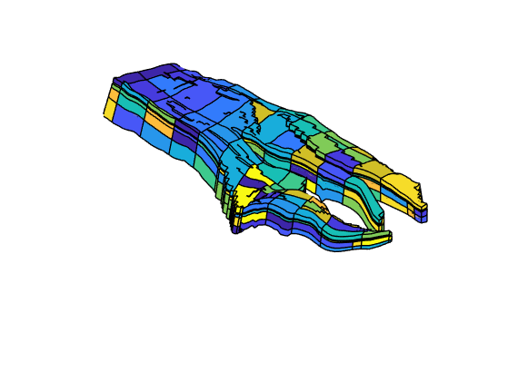
Set up support regions required for MsRSB and move center points to wells

CG = coarsenGeometry(CG);
CG = addCoarseCenterPoints(CG);
CG = setCentersByWells(CG, W);
CG = storeInteractionRegion(CG, 'ensureConnected', true);
CG = setupMexInteractionMapping(CG);

Handled coarse block 1 / 277
Handled coarse block 2 / 277
Handled coarse block 3 / 277
Handled coarse block 4 / 277
Handled coarse block 5 / 277
Handled coarse block 6 / 277
Handled coarse block 7 / 277
Handled coarse block 8 / 277
...

Set up basis functions

By default, we use the C-accelerated version

useCompiledBasis = true;
A = getIncomp1PhMatrix(G, T);
% Update basis functions every now and then
updateBasis = true;

getBasis = @(A) getMultiscaleBasis(CG, A, 'type', 'MsRSB', 'useMex', useCompiledBasis);
basis0 = getBasis(A);

Recieved 9 input arguments and requested 1 outputs
Matlab matrix processed in 5 ms
Discovered problem with 44915 cells and 277 blocks
Problem has 44915 equations with up to 20 connections and support in 481664 cells total.
Max number of threads: 8
Creating mappings...
Starting basis generation...
Starting smoothing iterations... done after 125 iterations.
...

Solve multiscale without iterations

We solve the base case where only the multiscale solver is used.

basis = basis0;
W_ms = W;
fn = getSmootherFunction('type', 'ilu');

psolve = @(state, basis) incompMultiscale(state, CG, T, fluid, basis, 'wells', W_ms, ...
    'getSmoother', fn, 'iterations', 0);

states_ms([1 N_step+1]) = psolve(state0, basis);
for i = 1:N_step
    state = states_ms(end);

    if updateBasis && mod(i, 10) == 0 && i > 1
        A = getIncomp1PhMatrix(G, T, state, fluid);
        basis = getBasis(A);
    end

    fprintf('Step %d of %d: ', i, N_step);
    fprintf('Solving pressure...
');
    state = psolve(state, basis);
    fprintf('Ok! ');
    fprintf('Solving transport...
');
    states_ms(i+1) = solver(state);
    fprintf('Ok!\n');
end

Step 1 of 100: Solving pressure... Ok! Solving transport... Ok!
Step 2 of 100: Solving pressure... Ok! Solving transport... Ok!
Step 3 of 100: Solving pressure... Ok! Solving transport... Ok!
Step 4 of 100: Solving pressure... Ok! Solving transport... Ok!
Step 5 of 100: Solving pressure... Ok! Solving transport... Ok!
Step 6 of 100: Solving pressure... Ok! Solving transport... Ok!
Step 7 of 100: Solving pressure... Ok! Solving transport... Ok!
Step 8 of 100: Solving pressure... Ok! Solving transport... Ok!
...

Solve using multiscale with additional iterations

We can apply 5 multiscale-ILU(0) cycles at each step in order to improve the solution quality at a low cost. The pressure is still far from converged, but this will help the solver to get the impact of wells correctly.

psolve = @(state, basis) incompMultiscale(state, CG, T, fluid, basis, 'wells', W_ms, ...
    'getSmoother', fn, 'iterations', 5, 'useGMRES', true);
basis = basis0;

states_it([1 N_step+1]) = psolve(state0, basis);
for i = 1:N_step
    state = states_it(end);
    if updateBasis && mod(i, 10) == 0 && i > 1
        A = getIncomp1PhMatrix(G, T, state, fluid);
        basis = getBasis(A);
    end

    fprintf('Step %d of %d: ', i, N_step);
    fprintf('Solving pressure...
');
    state = psolve(state, basis);
    fprintf('Ok! ');
    fprintf('Solving transport...
');
    states_it(i+1) = solver(state);
    fprintf('Ok!\n');
end

Step 1 of 100: Solving pressure... Ok! Solving transport... Ok!
Step 2 of 100: Solving pressure... Ok! Solving transport... Ok!
Step 3 of 100: Solving pressure... Ok! Solving transport... Ok!
Step 4 of 100: Solving pressure... Ok! Solving transport... Ok!
Step 5 of 100: Solving pressure... Ok! Solving transport... Ok!
Step 6 of 100: Solving pressure... Ok! Solving transport... Ok!
Step 7 of 100: Solving pressure... Ok! Solving transport... Ok!
Step 8 of 100: Solving pressure... Ok! Solving transport... Ok!
...

Set up interactive plotting of reservoir states

names = {'Finescale', 'MsRSB', 'MsRSB (5 cycles)'};

close all; plotToolbar(G, states);
axis equal tight off
daspect([1 1 0.2])
view(85, 20);
plotWell(G, W);
title(names{1});
colorbar('horiz')

figure; plotToolbar(G, states_ms);
axis equal tight off
daspect([1 1 0.2])
view(85, 20);
plotWell(G, W);
title(names{2});
colorbar('horiz')

figure; plotToolbar(G, states_it);
axis equal tight off
daspect([1 1 0.2])
view(85, 20);
plotWell(G, W);
title(names{3});
colorbar('horiz')

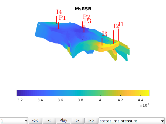
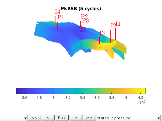
Launch interactive plotting of wells

Time = cumsum([0; repmat(dt, N_step, 1)]);

ws_ref = convertIncompWellSols(W, states, fluid);
ws_ms = convertIncompWellSols(W, states_ms, fluid);
ws_it = convertIncompWellSols(W, states_it, fluid);

ws = {ws_ref, ws_ms, ws_it};
shortname = {'ref', 'ms', 'it'};
plotWellSols(ws, Time, 'datasetnames', names)