`upscaling`: Upscaling of reservoir problems¶

Functionality and tutorials for averaging and upscaling permeability, transmissibility, relative permeability, etc.

Contents¶

UPSCALING Solvers for permeability upscaling problem

Files: computeMimeticIPGp - Wrapper for computeMimeticIP for periodic grids. computeTransGp - Wrapper for computeTrans for periodic grids. makeMatchingGridFromGrdel - { makePeriodicGridMulti3d - Construct a periodic grid. simulateToSteadyState - Simulate until steady state is reached upscaleGridRockAndWells - [rock_cg,CG,W_cg] = upscaleGridRockAndWells(G,rock,coarseDim) upscalePC - { upscalePCCaplimit - { upscalePerm - Compute upscaled permeabilites using flow based upscaling. upscalePermeabilityFixed - function for doing permeability upscaling on grids with fixed pressure conditions (pressure drop in one direction and noflow elsewhere) upscalePermeabilityMim - function for doing permeability upscaling on periodic grids upscalePermeabilityPeriodic - function for doing permeability upscaling on periodic grids upscaleRelperm - Upscale relative permeability. upscaleRelpermLimit - Upscale relperm based on viscous/capillary limit tabulated by saturation upscaleTrans - Calculate upscaled transmissibilities for a coarse model

computeMimeticIPGp(G, Gp, rock, varargin)¶: Wrapper for computeMimeticIP for periodic grids.

computeTransGp(G, Gp, rock)¶: Wrapper for computeTrans for periodic grids.

makePeriodicGridMulti3d(G, bcl, bcr, dprl, varargin)¶: Construct a periodic grid. G grid, bcl left boundary conditions, bcr right boundary conditions, dprl delta pressure over periodic edges

simulateToSteadyState(state, G, rock, fluid, dt, varargin)¶

Simulate until steady state is reached

Synopsis:

[state, report] = simulateToSteadyStatePeriodic(state, G, rock, fluid, dt)
[state, report] = simulateToSteadyStatePeriodic(state, G, rock, fluid, dt, 'pn', pv,...)

Parameters:

state – Reservoir and well solution structure either properly initialized from functions ‘initResSol’ and ‘initWellSol’ respectively, or the results from a previous call to function ‘incompTPFA’ and, possibly, a transport solver such as function ‘implicitTransport’.
G – Valid grid structure, see grid_structure.
rock – Rock containing fields ‘poro’ and ‘perm’.
dt – Initial time step used while trying to reach steady state. The time steps will be increased if the changes are miniscule during each timestep.
fluid – Fluid object.
Contains –
'pn'/pv – List of ‘key’/value pairs defining optional parameters. The supported options are:
fluid_nc – Fluid without capillary pressure. Will remove capillary pressure from fluid argument if not provided.
psolver – @(state,fluid) function handle to pressure solver.
bc – Boundary conditions
bcp – Periodic boundary conditions (if the grid is periodic)
solve_pressure – Pressure is solved each iteration
dt_max – Maximum time step allowed.
diff_tol – The tolerance used for checking if stationary state has been found.
<other> – Passed onto implicitTransport. Look there for explanations of the various parameters.

Returns:

state – Steady state.

COMMENTS:

Examples¶

Harmonic Upscaling of Realistic Field Model¶

Generated from cpGridHarmonic.m

Load the required modules

mrstModule add upscaling coarsegrid

Load and process data¶

We assume that the data has been downloaded and placed in the appropriate data directory under the MRST root directory.

saigupPath = fullfile(getDatasetPath('SAIGUP'), 'SAIGUP.GRDECL');
grdecl = readGRDECL(saigupPath);
grdecl = convertInputUnits(grdecl, getUnitSystem('METRIC'));
G      = processGRDECL(grdecl);
G      = computeGeometry(G);
rock   = grdecl2Rock(grdecl, G.cells.indexMap);

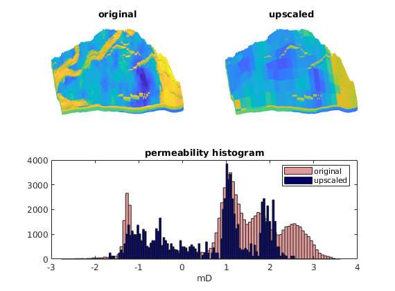
Upscale model¶

Upscale the model by a factor 5x5x5 using a simple harmonic average for the permeability and arithmetic average for the porosity. (This demonstrates the power of the accumarray call..)

w  = G.cells.volumes;
p  = partitionUI(G, G.cartDims./[5 5 5]);
for i=1:size(rock.perm,2)
   K = accumarray(p,w./rock.perm(:,i))./accumarray(p,w);
   crock.perm(:,i) = 1./K;
end
crock.poro = accumarray(p, rock.poro.*w)./accumarray(p,w);

Visualize result¶

As expected, using such a naive upscaling will move the permeability values towards the centre of their fine-scale spectre.

clf
pargs = {'EdgeColor','none'};
subplot(2,2,1)
plotCellData(G,log10(rock.perm(:,1)),pargs{:});
view(-95,40); axis tight off; cx = caxis; title('original');

subplot(2,2,2)
plotCellData(G, log10(crock.perm(p,1)), pargs{:});
set(gca,'zdir','reverse');
view(-95,40); axis tight off; caxis(cx); title('upscaled');

subplot(2,2,3:4)
hist(log10(convertTo(rock.perm(:,1),milli*darcy)), 100);
hold on
hist(log10(convertTo(crock.perm(p,1),milli*darcy)), 100);
hold off
h=get(gca,'Children');
set(h(1),'FaceColor',[0 0 0.4])
set(h(2),'FaceColor',[0.7 0 0],'FaceAlpha',.4)
legend('original','upscaled');
title('permeability histogram'); xlabel('mD')

Copyright notice¶

<html>
% <p><font size="-1

Steady-state permeability upscaling¶

Generated from periodicUpscaleExample.m

This example demonstrates upscaling of relative permeability on periodic grids. To this end, we upscale a single block sampled from SPE10 using first a standard flow-based method to determine the effective permeability and then finds relative permeability curves based on steady-state upscaling for the capillary and the viscous limits, as well as based on a dynamic simulation.

% Load the required modules
mrstModule add mimetic upscaling spe10 incomp deckformat

Set up a simple grid with periodic boundaries¶

Make a grid in which the right boundary wraps around with left boundary, the front with the back, and the bottom with the top. We retain the regular grid for plotting, as plotGrid uses the boundary faces to plot grids: A fully periodic grid has, per definition, no boundary faces.

G   = cartGrid([5 5 2]);
G   = computeGeometry(G);

% Set faces for wrap-around
bcr{1}=pside([],G,'RIGHT',0);   bcl{1}=pside([],G,'LEFT',0);
bcr{2}=pside([],G,'FRONT',0);   bcl{2}=pside([],G,'BACK',0);
bcr{3}=pside([],G,'BOTTOM',0);  bcl{3}=pside([],G,'TOP',0);

% Make periodic grid.
[Gp, bcp]=makePeriodicGridMulti3d(G, bcl, bcr, {0, 0, 0});

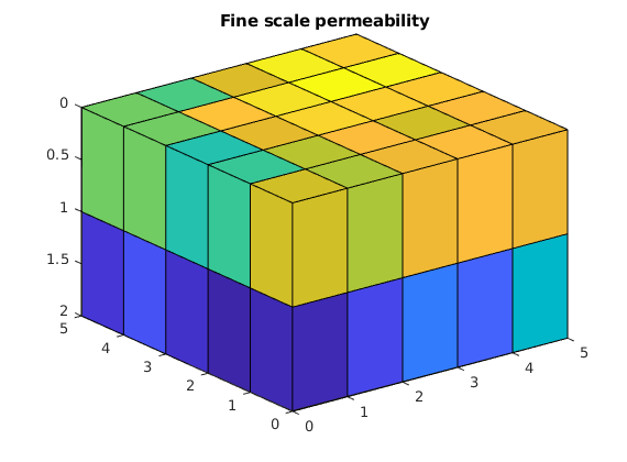
Extract a small subset of SPE10 to upscale.¶

x = 51; y = 11; z = 1;

rock = getSPE10rock(x:(x-1+G.cartDims(1)),...
                    y:(y-1+G.cartDims(2)),...
                    z:(z-1+G.cartDims(3)));
rock.perm = convertTo(rock.perm, milli*darcy);

clf
plotCellData(G, log10(rock.perm(:,1))); view(3); axis tight
title('Fine scale permeability')

Do a single-phase periodic upscale¶

To find the permeability we use a unitary fluid so that the mobility/relperm is equal to the saturation which is equal to one, removing any fluid specific effects. We upscale the permeability using two-point flux approximation for the pressure solver.

psolver = @(state, Grid, Fluid, BCP, Rock)...
           incompTPFA(state, Grid, computeTransGp(G, Grid, Rock),...
           Fluid, 'bcp', BCP);
L = max(G.faces.centroids) - min(G.faces.centroids);
fluid_pure = initSingleFluid('mu',1,'rho',1);

warning('off', 'mrst:periodic_bc')
perm2 = upscalePermeabilityPeriodic(Gp, bcp, 1, psolver, fluid_pure, rock, L);
warning('on', 'mrst:periodic_bc')

Load a two-phase fluid for upscaling¶

The data are synthetic and should not be used for anything but testing. The file ‘rocklist.txt’ contains a list of included property files in a simple format tabulated on water saturation.

current_dir = fileparts(mfilename('fullpath'));
fn    = fullfile(current_dir, 'rocklist.txt');

T  = readTabulatedJFluidFile(fn);

% Print the tabulated values from the first and only file
fprintf('\n');
fprintf(' Sw          | Krw         | Kro         | J-func\n')
fprintf('-------------|-------------|-------------|------------\n')
fprintf(' %+1.4e | %+1.4e | %+1.4e | %+1.4e\n', T{1} .')
fprintf('\n');

fluid = initSWOFFluidJfunc('mu' , [   10,  100] .* centi*poise     , ...
                             'rho', [1000, 600] .* kilogram/meter^3, ...
                             'table', T, ...
                             'satnum', 1, 'jfunc', true, 'rock', rock, ...
                             'surf_tens', 10*dyne/(centi*meter));

Sw          | Krw         | Kro         | J-func
-------------|-------------|-------------|------------
 +1.6380e-01 | +0.0000e+00 | +1.0510e+00 | +2.3538e+00
 +2.0870e-01 | +1.7000e-02 | +9.6900e-01 | +2.2030e-01
 +2.4530e-01 | +1.7500e-02 | +8.1380e-01 | +1.1690e-01
 +2.7820e-01 | +1.8300e-02 | +6.6210e-01 | +8.8500e-02
 +3.0570e-01 | +1.9000e-02 | +5.3770e-01 | +7.6600e-02
...

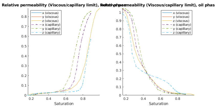
Steady-state upscaling (viscous/capillary limits)¶

We assume zero capillary forces and do a steady-state upscale using the viscous and capillary limits, respectively. The viscous limit is equal in all directions, while the capillary is not

[saturations_visc, kr_visc] = ...
   upscaleRelpermLimit(G, rock, fluid, 'type', 'fixed', 'limit', 'viscous');
[saturations_cap, kr_cap]   = ...
   upscaleRelpermLimit(G, rock, fluid, 'type', 'fixed', 'limit', 'capillary');

% Plot the results
clf;
p = get(gcf,'Position'); set(gcf,'Position',[p(1:2) 840 420]);
ph = {'water', 'oil'};
for i = 1:2
    subplot(1,2,i)
    hold on
    plot(saturations_visc, kr_visc{i});
    plot(saturations_cap, kr_cap{i}, '--.');
    title(['Relative permeability (Viscous/capillary limit), ' ph{i} ' phase']);
    hold off; axis tight
    xlabel('Saturation')
    legend({'x (viscous)', 'y (viscous)', 'z (viscous)'...
            'x (capillary)', 'y (capillary)', 'z (capillary)'}, 'location', 'Best')
end

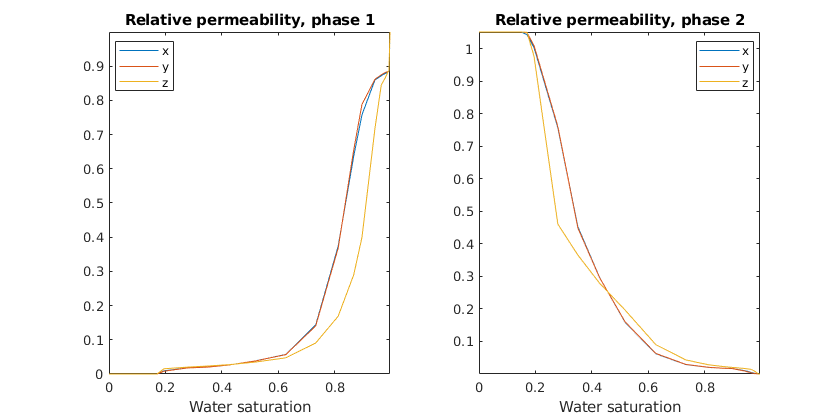
General steady-state upscaling¶

In the general case, we initialize the model with a certain fraction of water and simulate the dynamic behaviour due to a linear pressure drop in until steady-state is reached. This way, we can tabulate relative permeability versus average water saturation. Here, we use ~20 data points. As the default option is to use a pressure drop in x-direction, the x-values are significantly different from the y/z values which are similar, but not equal.

saturations = 0:0.05:1;
dp_scale=1e-3;

% Ignore warnings from the implicit solver as the solution is driven to
% steady state. It is natural that some steps fail during this process.
warning('off', 'implicitTransport:failure')
[sat_vec, kr, perm, krK] = upscaleRelperm(G, rock, fluid, dp_scale, saturations, 'periodic', false);
warning('on', 'implicitTransport:failure')

% Plot the resulting relative permeability
for i = 1:2
   subplot(1,2,i)
   plot(sat_vec, kr{i});
   title(['Relative permeability, phase ' num2str(i)]);
   axis tight
   xlabel('Water saturation')
   legend({'x', 'y', 'z'}, 'location', 'Best')
end

implicitTransport: FAILED due to timestep 4.73987 < 9.47975.
implicitTransport: FAILED due to timestep 0.592484 < 4.73987.
implicitTransport: FAILED due to timestep 9.47975 < 18.9595.
implicitTransport: FAILED due to timestep 2.36994 < 9.47975.
implicitTransport: FAILED due to timestep 2.36994 < 4.73987.
implicitTransport: FAILED due to timestep 9.47975 < 18.9595.
implicitTransport: FAILED due to timestep 2.36994 < 9.47975.
implicitTransport: FAILED due to timestep 0.296242 < 0.592484.
...

Copyright notice¶

<html>
% <p><font size="-1

unction [kr]=simpleRelpermUpscalingExample2D(perm_case,fluid_case)
% This demonstrate the method used for relperm upscaling
%  The default setup is a quasi 1D case

mrstModule add mimetic upscaling incomp

warning('off','mrst:periodic_bc');
figure(3),clf
if(nargin==0)
    perm_case='uniform';
    fluid_case='periodic_capillary_pressure';
end
% set up grid
Lx = 10; Ly = 10;
nx = 50; ny = 2;
G = cartGrid([nx ny], [Lx Ly]);
G = computeGeometry(G);
sperm = 100;
%
rock=makePerm(perm_case,G);
n =  [2 2]; %set original exponent of fluid
mu = [1 4]; %set viscosity of fluids

[fluid_pure,fluid,fluid_nc] = makeFluids(fluid_case,rock,G,Lx,Ly,'n',n,'mu',mu);
dp_scale = 4*barsa;
dpx = dp_scale;
dpy = 0.0;
% set the saturations to be upscaled
sat_vec = 0.1:0.2:0.9;

%%%%%%%%%%%%%%%%%%%%%%%%%%%%%%%%%%%%%%%%%%%%%%%%%%%%%%%%%%%%%%%%%%%%%%%%%%
% Upscale using MRST upscaling
%%%%%%%%%%%%%%%%%%%%%%%%%%%%%%%%%%%%%%%%%%%%%%%%%%%%%%%%%%%%%%%end%%%%%%%%%%
[sat_mat, kr, perm, krK] = upscaleRelperm(G, rock, fluid, dp_scale,...
                                     sat_vec, 'periodic', true, 'dir', 1); %#ok<NASGU,ASGLU>
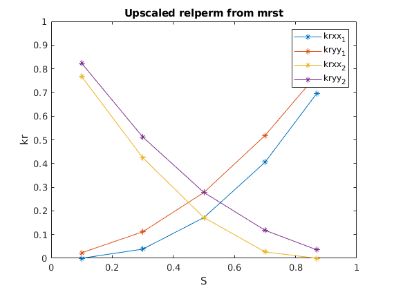
% plot the result
figure(1),clf
plot(sat_mat,[kr{1}(:,[1,4]),kr{2}(:,[1,4])],'*-')
legend('krxx_1','kryy_1','krxx_2','kryy_2')
xlabel('S')
ylabel('kr')
axis([0 1 0 1])
title('Upscaled relperm from mrst')

%%%%%%%%%%%%%%%%%%%%%%%%%%%%%%%%%%%%%%%%%%%%%%%%%%%%%%%%%%%%%%%%%%%%%%%%%%%
% Start example of upscaling
%%%%%%%%%%%%%%%%%%%%%%%%%%%%%%%%%%%%%%%%%%%%%%%%%%%%%%%%%%%%%%%%%%%%%%%%%%%
% define pressure drop
bl=pside([],G,'LEFT',0);
br=pside([],G,'RIGHT',0);
bd=pside([],G,'BACK',0);
bu=pside([],G,'FRONT',0);


% find boundary cells which are used to calculate fluxes
cells_r=sum(G.faces.neighbors(br.face,:),2);
%cells_u=sum(G.faces.neighbors(bu.face,:),2);

% make periodic grid
[Gp,bcp]=makePeriodicGridMulti(G,{bl,bd},{br,bu},{dpx,dpy});
Trans = computeTrans(G,rock);
Transp = Trans(Gp.cells.faces(:,end));

phase_fluxkr = nan(numel(sat_vec),2);
lambda = @(s) bsxfun(@rdivide,fluid.relperm(s),fluid.properties());

% initialize state and calculate trivial upscaling
state = initResSol(Gp, 100*barsa, 1);
state = incompTPFA(state,Gp,Transp,fluid_pure,'bcp',bcp);
x_faces = bcp.face(bcp.value==dpx);
%y_faces=bcp.face(bcp.value==dpy);
sign_x = 2*(Gp.faces.neighbors(x_faces,1)==cells_r)-1;
%sign_y=2*(Gp.faces.neighbors(y_faces,2)==cells_u)-1;
tflux_x = sum(state.flux(x_faces).*sign_x);
%tflux_y=sum(state.flux(y_faces).*sign_y);
tflux = tflux_x;
permkr = (tflux/Ly)/(dpx/Lx);
DT = 100*day;

% set up parmeter used in the uspcaling lop
max_DT = 40*year;
max_it = 40;
diff_tol = 1e-4;

%%%%%%%%%%%%%%%%%%%%%%%%%%%%%%%%%%%%%%%%%%%%%%%%%%%%%%%%%%%%%%%%%%%%%%%%%%%
% Start loop for finding upcaled relperm
%%%%%%%%%%%%%%%%%%%%%%%%%%%%%%%%%%%%%%%%%%%%%%%%%%%%%%%%%%%%%%%%%%%%%%%%%%%
state=initResSol(Gp, 100*barsa, 0.1);
pv=poreVolume(G,rock);
for i=1:numel(sat_vec);
   sat=sat_vec(i);
   % errir ub treatment of boundary conditions
   %fl_sat=lambda(sat);
   %fl_sat=fl_sat(:,1)/sum(fl_sat,2);


   % make initial saturation to for the statoinary state calculation
   eff_sat=sum(state.s.*pv)/sum(pv);
   if(eff_sat > 0 )
        state.s=state.s*(sat/eff_sat);
   else
        state.s=ones(size(state.s))*sat;
   end
   state.s=ones(size(state.s))*sat;
   % search for stationary state
   init_state=state;
   it=0;
   stationary=false;
%%%%%%%%%%%%%%%%%%%%%%%%%%%%%%%%%%%%%%%%%%%%%%%%%%%%%%%%%%%%%%%%%%%%%%%%%%%
% Start loop for finding stationary state
%%%%%%%%%%%%%%%%%%%%%%%%%%%%%%%%%%%%%%%%%%%%%%%%%%%%%%%%%%%%%%%%%%%%%%%%%%%
% find a flux assosiated with the pressure drop

   state=incompTPFA(state,Gp,Transp,fluid_nc,'bcp',bcp);
   while ~stationary && it < max_it
      s_pre=state.s;
      % do one transport step
       [state,report]=implicitTransport(state,Gp,DT,rock,fluid,'Trans',Transp,...
                  'verbose',false,...
                    'nltol'   ,         1.0e-6, ...
 % Non-linear residual tolerance
                'lstrials',         10    , ...
 % Max no of line search trials
              'maxnewt' ,         20    , ...
 % Max no. of NR iterations
              'tsref'   ,         4    , ...
 % Time step refinement
              'init_state',init_state);

      disp(['Iteration ',num2str(it),' DT ', num2str(DT/year),' Error ', num2str(norm(s_pre-state.s))])
      % check if transport step is successfull
      if(report.success)
         init_state=state;
         % increas timestep if change is small
         if(norm(s_pre-state.s,inf)<1e-2)
            DT=min(max_DT,DT*2);
         end
         % calculate new pressure
         state=incompTPFA(state,Gp,Transp,fluid,'bcp',bcp);
         if(norm(s_pre-state.s,inf)<diff_tol)
            stationary=true;
         end
      else
         % if not success full cut time step
         disp('Cutting time step');
         init_state.s=0.5*ones(size(state.s));
         DT=DT/2;
      end
      it=it+1;
   end

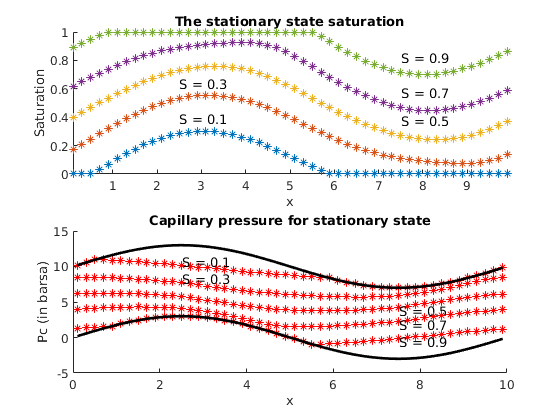
   % Plot the stationary state
   %
   figure(3)
   pv=poreVolume(G,rock);
   sat_vec(i)=sum(pv.*state.s(:,1))/sum(pv);

   if(ny>2)
      clf,plotCellData(G,state.s),colorbar
   else
     %clf,
     mcells=1:nx;
       subplot(2,1,1),%cla
       hold on
       plot(G.cells.centroids(mcells,1),state.s(mcells),'*')
       axis([min(G.cells.centroids(:,1)) max(G.cells.centroids(:,1)), 0 1])
       ylabel('Saturation')
       xlabel('x');
       %title(['The stationary saturation for average saturation', num2str(sat_vec(i))])
       title('The stationary state saturation')
       if(sat_vec(i)<0.5)
        ind=floor(numel(mcells)/4)+1;
        text(G.cells.centroids(ind,1),state.s(ind,1)+0.1,['S = ', num2str(sat_vec(i))])
       else
        ind=floor(3*numel(mcells)/4)+1;
        text(G.cells.centroids(ind,1),state.s(ind,1)+0.1,['S = ', num2str(sat_vec(i))])
       end


       subplot(2,1,2),%cla

       hold on
       % calculate capillary pressure for plotting
       mpc=fluid.pc(state);
       % calculate capillary pressure if saturation is zero or one
       mpc0=fluid.pc(struct('s',zeros(G.cells.num,1)));
       mpc1=fluid.pc(struct('s',ones(G.cells.num,1)));
       plot(G.cells.centroids(mcells,1),mpc0(mcells)/barsa,'k','LineWidth',2)
       plot(G.cells.centroids(mcells,1),mpc(mcells)/barsa,'r*')
       plot(G.cells.centroids(mcells,1),mpc1(mcells)/barsa,'k','LineWidth',2)
       ylabel('Pc (in barsa)')
       xlabel('x');
       %title(['Capillary pressure for stationary state with average saturation', num2str(sat_vec(i))])
       title('Capillary pressure for stationary state')
       if(sat_vec(i)<0.5)
        ind=floor(numel(mcells)/4)+1;
         text(G.cells.centroids(ind,1),mpc(ind,1)/barsa+0.5,['S = ', num2str(sat_vec(i))])
       else
           ind=floor(3*numel(mcells)/4)+1;
         text(G.cells.centroids(ind,1),mpc(ind,1)/barsa-0.5,['S = ', num2str(sat_vec(i))])
       end
       %axis([min(G.cells.centroids(:,1)) max(G.cells.centroids(:,1)), 0 1])

   end
   drawnow;
   % calculate new correct fluxes
   state=incompTPFA(state,Gp,Transp,fluid,'bcp',bcp);
   % store if the upscaling has been success full or not
   if(~stationary)
      sim_ok(i)=false;%#ok
   else
      sim_ok(i)=true;%#ok
   end
   % do single phase upscaling solves to find Kkr
   lam= lambda(state.s);
   Ts={};rocks={};states={};
   for kk=1:2;
      rocks{kk}.perm=rock.perm.*lam(:,kk);%#ok
      Ts{kk} = computeTrans(G,rocks{kk});%#ok
      TT=Ts{kk}(Gp.cells.faces(:,3));
      TT(TT==0)=1e-6*max(TT);
      states{kk}=incompTPFA(state,Gp,TT,fluid_pure,'bcp',bcp); %#ok
   end
   phase_fluxkr(i,:)=[sum(states{1}.flux(x_faces).*sign_x),sum(states{2}.flux(x_faces).*sign_x)];
   disp(['Saturation ',num2str(sat)])
end

mu = fluid.properties();
upperm=permkr;
% compare the upscaled permeability with the original
disp(['Upscaled perm is ', num2str(upperm/(milli*darcy)),...
   ' input was ', num2str(sperm)])

% plot the upscaled relperms.
% the result below depend on that upscaled permeability is scalar
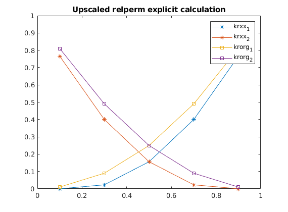
figure(2)
ir_up=bsxfun(@rdivide,bsxfun(@times,phase_fluxkr,mu),(upperm*dpx*Ly/Lx));
%clf,plot(sat_vec,ir_up,'bx-',sat_vec,fluid.relperm(sat_vec')','r');
clf,plot(sat_vec,ir_up,'*-',sat_vec,fluid.relperm(sat_vec')','s-');
legend('krxx_1','krxx_2','krorg_1','krorg_2')
hold on
plot(sat_vec(~sim_ok),ir_up(~sim_ok,:),'ro')
axis([0 1 0 1])
title('Upscaled relperm explicit calculation')

disp(['Upscaled perm is ', num2str(permkr/(milli*darcy)),...
   ' should be ', num2str(sperm)])
if(ny>2)
    figure(3)
    clf,plotCellData(G,log(rock.perm/(milli*darcy))),colorbar
    title('permeability')
end
kr=[sat_vec',ir_up];
end

%%%%%%%%%%%%%%%%%%%%%%%%%%%%%%%%%%%%%%%%%%%%%%%%%%%%%%%%%%%%%%%%%%%%%%%%%%%
% help functions to set ups several test cases and fluid is below here
%%%%%%%%%%%%%%%%%%%%%%%%%%%%%%%%%%%%%%%%%%%%%%%%%%%%%%%%%%%%%%%%%%%%%%%%%%%

function rock=makePerm(perm_case,G)
sperm=100*milli*darcy;
switch perm_case
    case 'uniform'
        rock.poro=0.1*ones(G.cells.num,1);
        rock.perm=sperm*ones(G.cells.num,1);
    case 'random'
        RandStream.setGlobalStream(RandStream('mt19937ar','seed',1));
        rock.perm=sperm*rand(G.cells.num,1);
        rock.poro=0.1*ones(G.cells.num,1);
    case 'brick'
        rock.perm=sperm*rand(G.cells.num,1);
        rock.poro=0.1*ones(G.cells.num,1);
        cell=sub2ind(G.cartDims,floor(nx/2)+1,floor(ny/2)+1);
        rock.perm(cell)=1e-4*rock.perm(cell);
    case 'chess'
        %RandStream.setDefaultStream(RandStream('mt19937ar','seed',1));
        %rock.perm=sperm*milli*darcy*rand(G.cells.num,1);
        rock.perm=sperm*ones(G.cells.num,1);
        rock.poro=0.1*ones(G.cells.num,1);
        % cell=sub2ind(G.cartDims,floor(nx/2)+1,floor(ny/2)+1);
        perm_tmp=reshape(rock.perm,G.cartDims);
        perm_tmp(:,1:2:end)=1e-4*perm_tmp(:,1:2:end);
        %perm_tmp(1:2:end,:)=1e-2*perm_tmp(1:2:end,:);
        rock.perm=perm_tmp(:);
        %rock.perm(cell)=1e-4*rock.perm(cell)
    case 'lognormal'
        RandStream.setGlobalStream(RandStream('mt19937ar','seed',1));
        rock.perm=logNormLayers(G.cartDims,'std',1)*sperm;
        rock.poro=0.1*ones(G.cells.num,1);
    otherwise
        error('No such permability field implemented');
end
end

%--------------------------------------------------------------------------

function [fluid_pure,fluid,fluid_nc]=makeFluids(fluid_case,rock,G,Lx,Ly,varargin)
opt=struct('mu',[1 1],'n',[1 1]);
opt=merge_options(opt,varargin{:});
fluid_pure = initSingleFluid('mu' ,  1    , ...
    'rho', 1);
switch fluid_case
    case 'pc_Simple'
        gravity off;
        fluid      = initSimpleFluidPc('mu' , [   1,   1]*centi*poise    , ...
            'rho', [1000,1000]*kilogram/meter^3, ...
            'n'  , [1 1],....
            'pc_scale',-1e2*barsa);
        fluid_nc=fluid;
    case 'ps_Jscaled'
        n=opt.n;
        mu=opt.mu;
        fluid      = initSimpleFluidJfunc('mu' , mu*centi*poise    , ...
            'rho', [1000,1000]*kilogram/meter^3, ...
            'n'  , n,....
            'surf_tension',-10*barsa/sqrt(0.1/(sperm*milli*darcy)),...
            'rock',rock);
        fluid_nc      = initSimpleFluidJfunc('mu' ,mu*centi*poise    , ...
            'rho', [1000,1000]*kilogram/meter^3, ...
            'n'  , n,....
            'surf_tension',-10*barsa/sqrt(0.1/(sperm*milli*darcy)),...
            'rock',rock);
    case 'periodic_capillary_pressure'
        n=opt.n;
        mu=opt.mu;
        fluid      = initSimpleFluidPeriodicPcMulti('mu' , mu*centi*poise    , ...
            'rho', [1000,1000]*kilogram/meter^3, ...
            'n'  , n,....
            'amplitude',10*barsa,...
            'G',G,...
            'L',[Lx,Ly]);
        fluid_nc=fluid;
    otherwise
        error('No such model')
end
end

%--------------------------------------------------------------------------

function fluid = initSimpleFluidPeriodicPcMulti(varargin)
%Initialize incompressible two-phase fluid model (analytic rel-perm).
%
% SYNOPSIS:
%   fluid = initSimpleFluid('pn1', pv1, ...)
%
% PARAMETERS:
%   'pn'/pv - List of 'key'/value pairs defining specific fluid
%             characteristics.  The following parameters must be defined
%             with one value for each of the two fluid phases:
%               - mu  -- Phase viscosities in units of Pa*s.
%               - rho -- Phase densities in units of kilogram/meter^3.
%               - n   -- Phase relative permeability exponents.
%
% RETURNS:
%   fluid - Fluid data structure as described in 'fluid_structure'
%           representing the current state of the fluids within the
%           reservoir model.
%
% EXAMPLE:
%   fluid = initSimpleFluid('mu' , [   1,  10]*centi*poise     , ...
%                           'rho', [1014, 859]*kilogram/meter^3, ...
%                           'n'  , [   2,   2]);
%
%   s = linspace(0, 1, 1001).'; kr = fluid.relperm(s);
%   plot(s, kr), legend('kr_1', 'kr_2')
%
% SEE ALSO:
%   `fluid_structure`, `solveIncompFlow

Warning: Matrix is close to singular or badly scaled. Results may be inaccurate.
RCOND =  1.837822e-20.
Warning: Matrix is close to singular or badly scaled. Results may be inaccurate.
RCOND =  1.047153e-21.
Warning: Matrix is close to singular or badly scaled. Results may be inaccurate.
RCOND =  1.837822e-20.
Warning: Matrix is close to singular or badly scaled. Results may be inaccurate.
RCOND =  1.047153e-21.
...

_images/simpleRelpermUpscalingExample2D_01.png

_images/simpleRelpermUpscalingExample2D_02.png

_images/simpleRelpermUpscalingExample2D_03.png

Single-phase upscaling¶

Generated from simpleUpscaleExample.m

This example demonstrates how to perform a single-phase upscaling of the absolute permeability for a 2D Cartesian model. The routines we use are also applicable in 3D.

% Load the required modules
mrstModule add upscaling coarsegrid mimetic incomp
verbose = true;

Define fine-scale model and coarse grid¶

We consider two different grids: a fine scale grid that represents the original model and a coarse-scale grid that represents the upscaled model in a way that is independent of the original fine-scale model. For the fine-scale model we define a lognormal permeability field.

cellDims  = [15 15 1];
G         = cartGrid(cellDims, cellDims);
G         = computeGeometry(G);
K         = exp( 5*gaussianField(cellDims, [-1 1], [7 7 1]) + 1);
rock.perm = convertFrom(K(:), milli()*darcy());

% The coarse grid
upscaled  = [5 5 1];
G_ups     = cartGrid(upscaled, cellDims);
G_ups     = computeGeometry(G_ups);

Compute upscaled permeability¶

To compute the upscaled permeability, we need to define a coarse-grid structure that describes how the coarse grid relates to the fine grid. In our case, this is simple: the coarse grid is uniform partition of the fine grid.

p  = partitionUI(G, upscaled);
p  = processPartition  (G, p);
CG = generateCoarseGrid(G, p, 'Verbose', verbose);

rockUps.perm = upscalePerm(G, CG, rock, 'Verbose', verbose);

Computing upscaled permeabilities... Elapsed time is 0.300814 seconds.

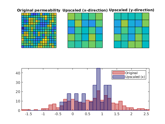
Plot permeabilities¶

Whereas the fine-scale permeability field is isotropic, the upscaled permeability field is anisotropic and we therefore plot both the components in both directions. In addition, we present a histogram of the original permeability and the upscaled permeability projected back onto the fine grid to more clearly show how upscaling reduces the span and tends to cluster values around the median of the fine-scale distribution.

clf
subplot(2,3,1)
plotCellData(G, log10(rock.perm));axis equal tight off
coaxis = caxis; title('Original permeability')

subplot(2,3,2)
plotCellData(G_ups, log10(rockUps.perm(:,1)));  axis equal tight off
title('Upscaled (x-direction)'); caxis(coaxis)

subplot(2,3,3)
plotCellData(G_ups,  log10(rockUps.perm(:,2)));  axis equal tight off
title('Upscaled (y-direction)'); caxis(coaxis)

subplot(2,3,4:6)
bins = -1.5:0.125:2.5;
hist(log10(rock.perm(:))-log10(milli*darcy),bins);
hold on;
hist(log10(rockUps.perm(p(:),1))-log10(milli*darcy),bins);
hold off
h=get(gca,'Children');
set(h(1),'EdgeColor',[0 0 0.4],'FaceColor',[0 0 .4],'FaceAlpha',.4);
set(h(2),'EdgeColor',[0.7 0 0],'FaceColor',[.7 0 0],'FaceAlpha',.4);
axis tight
legend('Original','Upscaled (x)');

Compare models¶

To compare the models, we set up a simple case with a unit pressure drop from south to north and compare the normal velocities on the outflow boundary to the north. Fluid parameters are typical for water.

fluid     = initSingleFluid('mu' ,    1*centi*poise     , ...
                            'rho', 1014*kilogram/meter^3);
% Fine-scale problem
bc        = pside([], G, 'North', 0);
faces     = bc.face;
bc        = pside(bc, G, 'South',  1*barsa());
T         = computeTrans(G, rock);
xRef      = incompTPFA(initResSol(G,0), G, T, fluid, 'bc', bc);

% Coarse-scale problem
bc_ups    = pside([], G_ups, 'North', 0);
faces_ups = bc_ups.face;
bc_ups    = pside(bc_ups, G_ups, 'South', 1*barsa());
T_ups     = computeTrans(G_ups, rockUps);
xUps      = incompTPFA(initResSol(G_ups,0), G_ups, T_ups, fluid, 'bc', bc_ups);

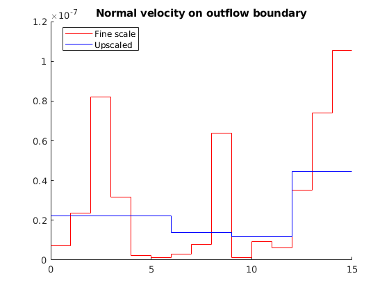
Compare outflow¶

The smoothing effect of the upscaling procedure is apparent. Whereas the total outflow is very close in the two models, we see that there is significant variation in the fine-scale model that is not captured by the coarse-scale model.

flux1 = sum(xRef.flux(faces));
flux2 = sum(xUps.flux(faces_ups));
disp(['Sum outflux on fine scale   : ', num2str(flux1)]);
disp(['Sum outflux on coarse scale : ', num2str(flux2)]);

flux1_face = xRef.flux(faces)    ./G.faces.areas(faces);
flux2_face = xUps.flux(faces_ups)./G_ups.faces.areas(faces_ups);
clf; hold on
x = G.faces.centroids(faces,1); dx = diff(x);
stairs([x-.5*dx(1); x(end)+.5*dx(end)], flux1_face([1:end end]), 'r-')
x = G_ups.faces.centroids(faces_ups,1); dx = diff(x);
stairs([x-.5*dx(1); x(end)+.5*dx(end)], flux2_face([1:end end]), 'b-')
hold off
title('Normal velocity on outflow boundary')
legend({'Fine scale', 'Upscaled'},'Location','best')

Sum outflux on fine scale   : 4.5395e-07
Sum outflux on coarse scale : 3.4345e-07

Copyright notice¶

<html>
% <p><font size="-1

upscaling: Upscaling of reservoir problems¶

Examples¶

Harmonic Upscaling of Realistic Field Model¶

Load and process data¶

Upscale model¶

Visualize result¶

Copyright notice¶

Steady-state permeability upscaling¶

Set up a simple grid with periodic boundaries¶

Extract a small subset of SPE10 to upscale.¶

Do a single-phase periodic upscale¶

Load a two-phase fluid for upscaling¶

Steady-state upscaling (viscous/capillary limits)¶

General steady-state upscaling¶

Copyright notice¶

Single-phase upscaling¶

Define fine-scale model and coarse grid¶

Compute upscaled permeability¶

Plot permeabilities¶

Compare models¶

Compare outflow¶

Copyright notice¶

`upscaling`: Upscaling of reservoir problems¶