`dg`: Discontinous Galerkin discretizations¶

Contents¶

MODELS

Files: TransportModelDG -

Contents¶

UTILS

Files: computeBoundaryFluxesDG - Undocumented Utility Function

computeBoundaryFluxesDG(model, state, bc)¶: Undocumented Utility Function

Contents¶

AD

Files: SpatialVector - Class for supporting ad as spatial vectors, for use in e.g.,

class SpatialVector(varargin)¶

Class for supporting ad as spatial vectors, for use in e.g., Discontinuous Galerkin discretizations

subsref(v, s)¶: Subscripted reference. Called for h = u(v).

times(u, v)¶: assert(all(size(u) == size(v)));

Contents¶

CUBATURES

Files: Cubature - Cubature class for cubatures on MRST grids LineCubature - 1D line cubatureature for faces in 2D MRST grids MomentFitting2DCubature - Cubature based on moment-fitting for MRST grids MomentFitting3DCubature - Cubature based on moment-fitting for MRST grids TetrahedronCubature - TriangleCubature - Triangle cubature class for cubatures on MRST grids

class Cubature(G, prescision, dim, varargin)¶

Cubature class for cubatures on MRST grids

Cubature(G, prescision, dim, varargin)¶: Setup up cubature properties. Acutual construction of cubature is handled by children class.

assignCubaturePointsAndWeights(cubature, x, w, n)¶: Assign points and weights

getCubature(cubature, elements, type, varargin)¶

Get cubature for given elements (either a set of cells or a set of faces) of the grid.

Keyword Arguments:
Parameters:	elements – Vector of cells or faces we want cubature for type – String equal to either * ‘volume’ : Volume integral, elements interpreted as cells ’face’ : Surface integral, elements interpreted as faces ’surface’: Surface integral over all faces of elements, which are interpreted as cells
	excludeBoundary – Exclude boundary faces in cell surface integrals internalConn – Boolean indicating what faces are internal connections, and therefore included in surface integrals. If empty, calculated from G.faces.neighbors outwardNormal – Surface integrals over cells are often on the form int(vdot n). outwardNormal = true changes signs based on face orientation so that normal points outwards.
Returns:	W – Integration matrix - integral = Wintegrand(x) x – Integration points cellNo, faceNo* – cell/face number telling what cubature point goes where

makeCubature(cubature)¶: #ok

transformCoords(cub, x, cells, inverse)¶

Transfor coordinates from physical to reference coordinates.

Parameters:	x – Coordinates in physical space cells – Cells we want reference coordinates for, cells(ix) are used when transforming x(ix,:) inverse – Boolean indicatiing if we are mapping to (inverse = false) or from (inverse = true) reference coordiantes. Default = false. useParent – Boolean indicating if we are working on the full grid (G.parent) or a subgrid.
Returns:	xhat – Transformed coordinates translation – Translation applied to x scaling – Scaling applied to x

G = None¶: Grid the cubature is defined on

dim = None¶: Dimension of cubature

internalConn = None¶: Boolean indicating if face is internal connection

numPoints = None¶: Number of cubature points

points = None¶: Cubature points

pos = None¶: Cubature points/weights for element e can be found

prescision = None¶: Prescision of cubature

weights = None¶: Cubature weights

class LineCubature(G, prescision)¶

1D line cubatureature for faces in 2D MRST grids

LineCubature(G, prescision)¶: Set up line cubatureature

makeCubature(cubature)¶: Make cubatureature

mapCoords(cubature, x, xR)¶: Map cubatureature points from reference to physical coordinates

class MomentFitting2DCubature(G, prescision, varargin)¶

Cubature based on moment-fitting for MRST grids

MomentFitting2DCubature(G, prescision, varargin)¶: Set up cubature

makeCubature(cubature)¶: Dimension of cubature

class MomentFitting3DCubature(G, prescision)¶

Cubature based on moment-fitting for MRST grids

MomentFitting3DCubature(G, prescision)¶: Set up cubatureature

makeCubature(cubature)¶: Dimension of cubature

class TriangleCubature(G, prescision)¶

Triangle cubature class for cubatures on MRST grids

TriangleCubature(G, prescision)¶: Set up triangle cubature

getTriAreas(cubature)¶: Get triangle areas

getTriangulation(cubature, G)¶: #ok Triangulate all cells or faces of G

makeCubature(cubature)¶: Make cubature

mapCoords(cubature, x, xR)¶: Map cubature points from reference to physical coordinates

mapCoordsBary(cubature, x)¶: Map cubature points from Barycentric to physical coordinates

triangulation = None¶: Struct containing triangulation information

Contents¶

DISCRETIZATIONS

Files: DGDiscretization - SpatialDiscretization -

Contents¶

STATEFUNCTIONS

Files: FluxDiscretizationDG -

Contents¶

FLOWPROPS

Files: MultipliedPoreVolumeDG - Effective pore-volume after pressure-multiplier

class MultipliedPoreVolumeDG(model, varargin)¶

Effective pore-volume after pressure-multiplier

evaluateOnDomain(prop, model, state)¶: Get effective pore-volume, accounting for possible rock-compressibility

Contents¶

FLUX

Files: ComponentPhaseVelocityFractionalFlowDG - ComponentTotalVelocityDG - FixedTotalFluxDG - FixedTotalVelocityDG - GravityPermeabilityGradientDG - GravityPotentialDifferenceDG - PhasePotentialUpwindFlagDG -

Examples¶

Buckley-Leverett displacement¶

Generated from dgExampleBLDisplacement.m

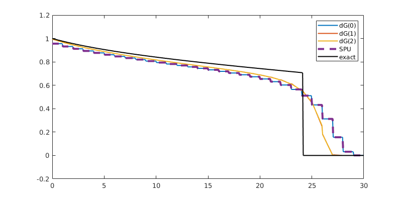
In this example, we consider an incompressible Buckley-Leverett displacement in a horizontal 1D channel aligned with the x-axis, and compare higher-order discontinuous Galerkin methods with the standard finite-volume discretization.

mrstModule add dg ad-core ad-props ad-blackoil blackoil-sequential
saveeps = @(a,b) disp(b);  % Dummy function

Set up problem¶

Construct grid, compute geometry and cell dimensions, and set petrophysical properties

G    = computeGeometry(cartGrid([30,1]));
G    = computeCellDimensions(G);
rock = makeRock(G, 1, 1);

% We consider Buckley-Leverett-type displacement with quadratic relperms
fluid = initSimpleADIFluid('phases', 'WO' , 'n', [2,2], ...
                           'mu', [1,1],  'rho', [1,1]);

% The base model is a generic black-oil model with oil and water
model  = GenericBlackOilModel(G, rock, fluid, 'gas', false);

% Initial state: filled with oil and unit volumetric flow rate
state0 = initResSol(G, 1, [0,1]);
state0.flux(1:G.cells.num+1) = 1;

% Boundary conditions
bc = fluxside([], G, 'left' ,  1, 'sat', [1,0]); % Inflow
bc = fluxside(bc, G, 'right', -1, 'sat', [1,0]); % Outflow

% Define schedule: unit time steps, simulate almost to breakthrough
schedule = simpleSchedule(ones(30,1), 'bc', bc);

Finite volume simulation¶

Use standard discretization in MRST: single-point upwind (SPU)

tmodel           = TransportModel(model);
[~, stFV, repFV] = simulateScheduleAD(state0, tmodel, schedule);

Solving timestep 01/30:            -> 1 Second
Solving timestep 02/30: 1 Second   -> 2 Seconds
Solving timestep 03/30: 2 Seconds  -> 3 Seconds
Solving timestep 04/30: 3 Seconds  -> 4 Seconds
Solving timestep 05/30: 4 Seconds  -> 5 Seconds
Solving timestep 06/30: 5 Seconds  -> 6 Seconds
Solving timestep 07/30: 6 Seconds  -> 7 Seconds
Solving timestep 08/30: 7 Seconds  -> 8 Seconds
...

Lowest-order dG simulation¶

Simulate using dG(0). This should be equivalent to SPU. The model is built as a wrapper around the base model, so that all physics are consistently handled by this. The base model is stored as the property ‘’parentModel’’

tmodelDG0 = TransportModelDG(model, 'degree', 0);
disp(tmodelDG0)

Getting supports.
Elapsed time is 0.078643 seconds.
Inverting systems...
  TransportModelDG with properties:

          discretization: [1×1 DGDiscretization]
             dgVariables: {'s'  'sW'  'sO'  'sT'}
                limiters: [2×1 struct]
...

Simulate dG(0)¶

[~, stDG0, repDG0] = simulateScheduleAD(state0, tmodelDG0, schedule);

Solving timestep 01/30:            -> 1 Second
Solving timestep 02/30: 1 Second   -> 2 Seconds
Solving timestep 03/30: 2 Seconds  -> 3 Seconds
Solving timestep 04/30: 3 Seconds  -> 4 Seconds
Solving timestep 05/30: 4 Seconds  -> 5 Seconds
Solving timestep 06/30: 5 Seconds  -> 6 Seconds
Solving timestep 07/30: 6 Seconds  -> 7 Seconds
Solving timestep 08/30: 7 Seconds  -> 8 Seconds
...

First-order dG simulation¶

TransportModelDG also takes optional arguments to DGDiscretization, such as degree. DGDiscretization supports using different polynomial order in each coordinate direction. We are simulating a 1D problem on a 2D grid, so we use higher order in the x-direction only.

tmodelDG1 = TransportModelDG(model, 'degree', [1,0]);

Getting supports.
Elapsed time is 0.041544 seconds.
Inverting systems...

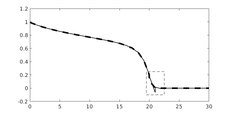
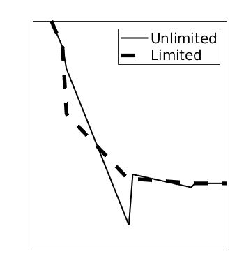
Limiters¶

Higher-order dG methods typically exhibit spurious oscillations near discontinuities. We countermand this with a limiter that effectively introduces enough numerical diffusion to dampen oscillations. We use two limiters by default: a TVB (Total Variation Bounded) limiter that adjusts the gradient whenever the jump across an interface is greater than 0, and a physical limiter that scales the solution so that the minimum and maximum in each cell is within physical limits. To see the limiters in action, we use ‘’afterStepFn’’ to plot the unlimited and limited solution after each timestep

tmodelDG1.storeUnlimited = true; % Store the unlimited state in each step
fn = plotLimiter(tmodelDG1, 'plot1d', true, 'n', 500); % afterStepFn

Simulate dG(1)¶

[~, stDG1, repDG1] = ...
    simulateScheduleAD(state0, tmodelDG1, schedule, 'afterStepFn', fn);

Solving timestep 01/30:            -> 1 Second
Solving timestep 02/30: 1 Second   -> 2 Seconds
Solving timestep 03/30: 2 Seconds  -> 3 Seconds
Solving timestep 04/30: 3 Seconds  -> 4 Seconds
Solving timestep 05/30: 4 Seconds  -> 5 Seconds
Solving timestep 06/30: 5 Seconds  -> 6 Seconds
Solving timestep 07/30: 6 Seconds  -> 7 Seconds
Solving timestep 08/30: 7 Seconds  -> 8 Seconds
...

Higher-order dG simulations¶

In principle, the dg module supports arbitrary order, as long as you can provide a sufficiently accurate quadrature rule. These are stored in e.g., ‘’getELEMENTCubaturePointsAndWeights’’, ELEMENT in {Triangle, Square, Tetrahedron, Cube}. We simulate the problem with dG(2)

tmodelDG2 = TransportModelDG(model, 'degree', [2,0]);
tmodelDG2.storeUnlimited = true;
fn = plotLimiter(tmodelDG2, 'plot1d', true, 'n', 500);

Getting supports.
Elapsed time is 0.038878 seconds.
Inverting systems...

Simulate dG(2)¶

[~, stDG2, repDG2] = ...
    simulateScheduleAD(state0, tmodelDG2, schedule, 'afterStepFn', fn);

Solving timestep 01/30:            -> 1 Second
Solving timestep 02/30: 1 Second   -> 2 Seconds
Solving timestep 03/30: 2 Seconds  -> 3 Seconds
Solving timestep 04/30: 3 Seconds  -> 4 Seconds
Solving timestep 05/30: 4 Seconds  -> 5 Seconds
Solving timestep 06/30: 5 Seconds  -> 6 Seconds
Solving timestep 07/30: 6 Seconds  -> 7 Seconds
Solving timestep 08/30: 7 Seconds  -> 8 Seconds
...

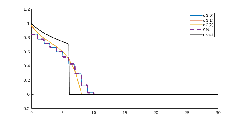
Compare results¶

Finally, we plot the results, and compare them to the exact solution

close all
% Plotting options
coords = getPlotCoordinates(G, 'n', 500, 'plot1d', true);    % Plot coords
opt    = {'linewidth', 1.5, 'coords', coords, 'plot1d', true}; % Plot options
s      = buckleyLeverettProfile('nW', 2, 'nN', 2);       % Exact sol
tsteps = [5,10,20]; % Timesteps

for t = tsteps
    figure('Position', [100, 100, 800, 400])
    % Tweak FV solution so we can plot it as dG
    stFV_plot      = stDG0{t};
    stFV_plot.sdof = stFV{t}.s;
    hold on
    plotSaturationDG(tmodelDG0.discretization, stDG0{t}, opt{:});
    plotSaturationDG(tmodelDG1.discretization, stDG1{t}, opt{:});
    plotSaturationDG(tmodelDG2.discretization, stDG2{t}, opt{:});
    plotSaturationDG(tmodelDG0.discretization, stFV_plot, ...
        'plot1d', true, 'coords', coords, 'linewidth', 3, 'lineStyle', '--');
    plot(coords.points(:,1), s(coords.points(:,1), t), 'linewidth', 1.5, 'color', 'k')
    hold off
    legend({'dG(0)', 'dG(1)', 'dG(2)', 'SPU', 'exact'});
    box on
    ylim([-0.2, 1.2])
end

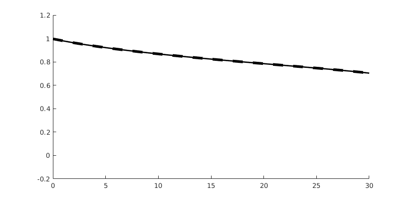
Plot dG(1) solution¶

close all
pos = [0,0,800,400];

figure('Position', pos)
t = 15;
hold on
    plotSaturationDG(tmodelDG1.discretization, stDG1{t}.ul, opt{:}, 'linewidth', 1.5, 'color', 'k');
    plotSaturationDG(tmodelDG1.discretization, stDG1{t}, opt{:}, 'linewidth', 4, 'color', 'k', 'linestyle', '--');
hold off
box on;
ylim([-0.2, 1.2])
ax = gca;
ax.FontSize = 14;
bx = [19.5, 22.5, -0.1, 0.25];
rectangle('Position', [bx([1,3]), bx([2,4]) - bx([1,3])], 'linestyle', '--');
drawnow(); pause(0.5), saveeps('buckley-leverett', 'limiter');

figure('Position', [0,0,350,400])
hold on
    plotSaturationDG(tmodelDG1.discretization, stDG1{t}.ul, opt{:}, 'linewidth', 1.5, 'color', 'k');
    plotSaturationDG(tmodelDG1.discretization, stDG1{t}, opt{:}, 'linewidth', 4, 'color', 'k', 'linestyle', '--');
hold off
box on;
axis(bx)
ax = gca;
ax.FontSize = 14;
[ax.XTick, ax.YTick] = deal([]);
legend({'Unlimited', 'Limited'}, 'fontSize', 15, 'Location', 'northeast')
drawnow(); pause(0.5), saveeps('buckley-leverett', 'limiter-zoom');

limiter
limiter-zoom

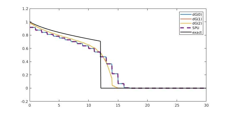
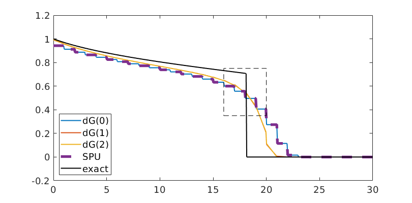
Compare FV and dG(0) - dG(2)¶

t = 15;
figure('Position', [100, 100, 800, 400])
% Tweak FV solution so we can plot it as dG
stFV_plot      = stDG0{t};
stFV_plot.sdof = stFV{t}.s;
hold on
plotSaturationDG(tmodelDG0.discretization, stDG0{t}, opt{:});
plotSaturationDG(tmodelDG1.discretization, stDG1{t}, opt{:});
plotSaturationDG(tmodelDG2.discretization, stDG2{t}, opt{:});
plotSaturationDG(tmodelDG0.discretization, stFV_plot, ...
    'plot1d', true, 'coords', coords, 'linewidth', 4, 'lineStyle', '--');
plot(coords.points(:,1), s(coords.points(:,1), t), 'linewidth', 1.5, 'color', 'k')
hold off
legend({'dG(0)', 'dG(1)', 'dG(2)', 'SPU', 'exact'}, 'fontsize', 14, 'location', 'southwest');
box on
ylim([-0.2, 1.2])
ax = gca;
ax.FontSize = 14;
bx = [16, 20, 0.35, 0.75];
rectangle('Position', [bx([1,3]), bx([2,4]) - bx([1,3])], 'linestyle', '--');
drawnow(); pause(0.5), saveeps('buckley-leverett', 'solutions')

figure('Position', [100, 100, 400, 400])
% Tweak FV solution so we can plot it as dG
stFV_plot      = stDG0{t};
stFV_plot.sdof = stFV{t}.s;
hold on
plotSaturationDG(tmodelDG0.discretization, stDG0{t}, opt{:});
plotSaturationDG(tmodelDG1.discretization, stDG1{t}, opt{:});
plotSaturationDG(tmodelDG2.discretization, stDG2{t}, opt{:});
plotSaturationDG(tmodelDG0.discretization, stFV_plot, ...
    'plot1d', true, 'coords', coords, 'linewidth', 4, 'lineStyle', '--');
plot(coords.points(:,1), s(coords.points(:,1), t), 'linewidth', 1.5, 'color', 'k')
hold off
box on
axis(bx)
ax = gca;
[ax.XTick, ax.YTick] = deal([]);
saveeps('buckley-leverett', 'solutions-zoom')

solutions
solutions-zoom

Components of a Discontinuous Galerkin Discretization in MRST¶

Generated from dgExampleDiscretization.m

This educational example goes through the main components of a discontinuous Galerkin (dG) discretization in MRST

mrstModule add dg
saveeps = @(a,b) disp(b);  % Dummy function
savepng = @(a,b) disp(b);  % Dummy function

Make grid¶

We construct a small PEBI grid

mrstModule add upr            % For generating PEBI grids
G = pebiGrid(1/8, [1,1]);     % PEBI grid
G = computeGeometry(G);       % Compute geometry
G = computeCellDimensions(G); % Compute cell dimensions

gray    = [1,1,1]*0.8; % For plotting
addText = @(x, string) text(x(:,1), x(:,2), string, 'fontSize', 12, 'HorizontalAlignment', 'left');

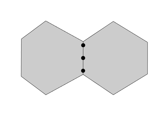
Plot the grid¶

We plot the grid and look at some geometric properties of a single cell

c = 22; % Cell number 17
% Plot cell 17 and its topological neighbors
figure();
plotGrid(G, 'facecolor', 'none');
cn = G.faces.neighbors(any(G.faces.neighbors == c,2),:);
cn = cn(cn>0);
plotGrid(G, cn(:), 'facecolor', 'none', 'linewidth', 2); axis equal off
plotGrid(G, c, 'facecolor', gray, 'linewidth', 2);
drawnow(), pause(0.2), saveeps('discretization', 'grid');
% By calling omputeCellDimensions(G), we computed the dimensions of a the
% smallest bounding box aligned with the coordinate axes so that the
% centroid of the box coincides with the cell centroid. We will use this to
% define our basis functions
xc = G.cells.centroids(c,:); % Centroid of cell 10
dx = G.cells.dx(c,:);        % Bounding box dimensions of cell 10
figure()
hold on
plotGrid(G, c, 'facecolor', gray);
rectangle('Position', [xc - dx/2, dx]);
plot(xc(1), xc(2), '.k', 'markerSize', 30);
plot([xc(1); xc(1)], [xc(2) - dx(2)/2; xc(2) + dx(2)/2], '--k');
plot([xc(1) - dx(1)/2; xc(1) + dx(1)/2], [xc(2); xc(2)], '--k');
axis equal off
drawnow(), pause(0.2), saveeps('discretization', 'cell');

grid
cell

Construct discretization¶

mrstModule add dg                        % Load module
G    = computeCellDimensions(G);         % Compute cell dimensions
disc = DGDiscretization(G, 'degree', 2); % Construct dG(2) discretization

Inspect basis¶

The basis functions are conveniently constructed by a Polynomial class. A polynomial is then described as a set of exponents k and weights w, and the class has overloaded operators for elementary arithmetic operations (addition, subtraction, multiplication, etc.), as well as tensor products, derivatives and gradients. We have construct a Legendre-type basis of polynomials of order <= 2.

disp(disc.basis)        % Inspect basis
disp(disc.basis.psi{3}) % The third basis function is simply y

psi: {6×1 cell}
    gradPsi: {6×1 cell}
     degree: 2
          k: [6×2 double]
       nDof: 6
       type: 'legendre'

  Polynomial with properties:
...

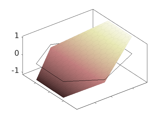
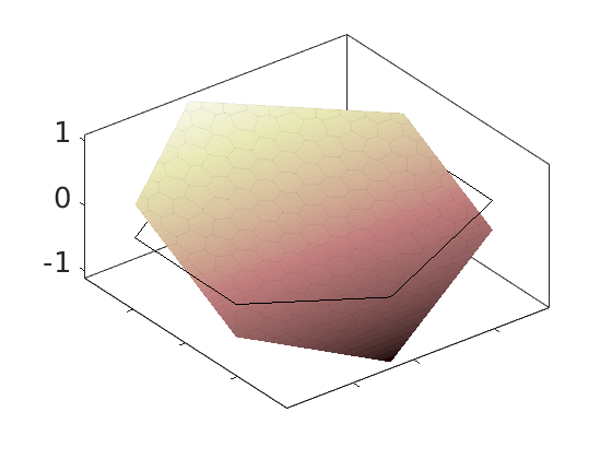
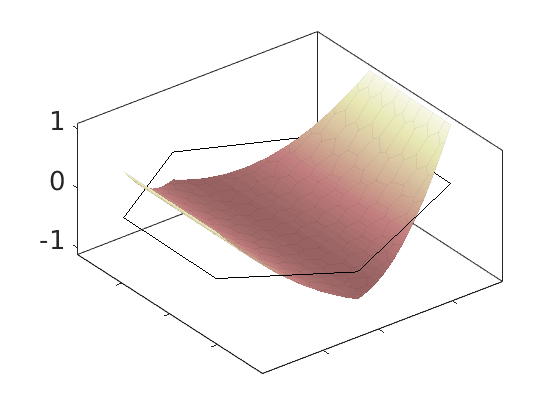
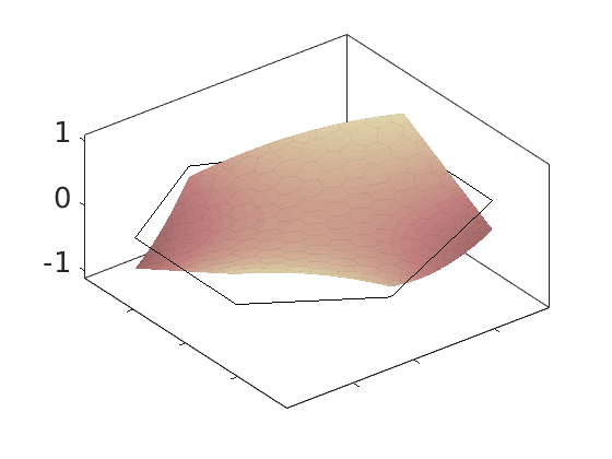
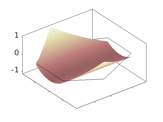
Plot polynomial basis¶

The basis functions are evaluated in local coordinates in each cell: $psi(hat{x}) = psi(frac{x - x_c}{Delta_x/2})

h = plotDGBasis(G, disc.basis, c, 'edgealpha', .05);
for i = 1:numel(h)
    set(0, 'CurrentFigure', h(i));
    ax = gca;
    [ax.XTickLabel, ax.YTickLabel] = deal({});
    ax.FontSize = 20; caxis([-1 1.2])
    savepng('discretization', ['basis-', num2str(i)]);
end

Warning: DistMesh did not converge in maximum number of iterations.
basis-1
basis-2
basis-3
basis-4
basis-5
basis-6

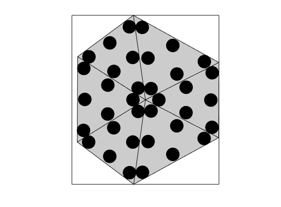
Construct triangle cubature¶

DG involves excessive evaluation of integrals. This is handeled by cubatures, which are implemented in the Cubature class. The simplest possible approach for polygonal cells is to subdivide the cells into simplices, and use a cubature rule for each simplex. This is implemented in the TriangleCUbature/TetrahedronCubature classes, which is the default cubature of the DGDiscretization

triCubature = disc.cellCubature;
figure(), plotCubature(G, triCubature, c, 'faceColor', gray); axis equal tight
savepng('discretization', 'cubature-tri');

cubature-tri

Test the triangle cubature¶

[W, x, ~, cells] = triCubature.getCubature(c, 'cell'); % Get points/weights
x = triCubature.transformCoords(x, cells); % Transform to reference coords
% The integral is easily evalauted using the matrix W, which has the
% cubature weights w placed so that int(psi)dx = W*psi(x). The weights sum
% to one, so that by construction, the integral of the first basis function
% (which is constant) should equal one, whereas the linear basis functions
% (1 and 2) should be zero
cellfun(@(psi) W*psi(x), disc.basis.psi)

ans =

    1.0000
    0.0000
    0.0000
   -0.1178
   -0.0006
...

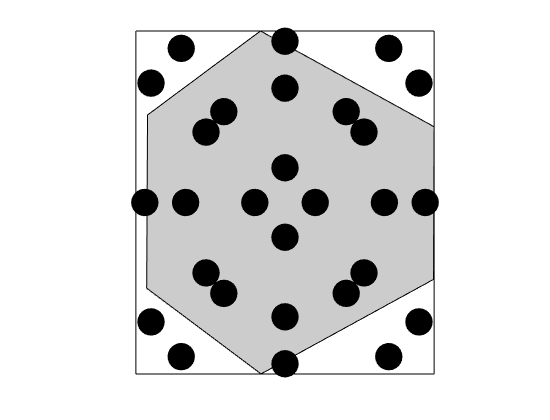
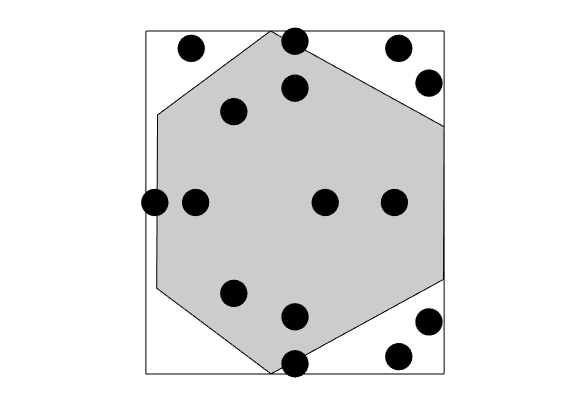
Construct moment fitting cubature¶

The cubature above uses much more points than strictly needed. We can construct a more efficient cubature by moment fitting. In this approach, we use a known cubature to compute the integrals for all functions in the basis for the polyomials we want our rule to be exact for. Then, given an initial set of cubature points, we compute corresponding weights by linear least squares, successively removing points until it is no longer possible to take away more points. In this case, the result is a cubature with six points, which equals the number of basis functions Moment-fitting without redcution

mrstModule add vem vemmech
degree = 2;
mfCubature_nr = MomentFitting2DCubature(G, 2*degree, 'chunkSize', 1, 'reduce', false);
figure(), plotCubature(G, mfCubature_nr, c, 'faceColor', gray); axis equal tight
savepng('discretization', 'cubature-mf-nr');
% Moment-fitting with redcution
mfCubature = MomentFitting2DCubature(G, 2*degree, 'chunkSize', 1);
figure(), plotCubature(G, mfCubature, c, 'faceColor', gray); axis equal tight
savepng('discretization', 'cubature-mf');

Compressing quadrature for element 1 to 1 of 87 ... Compressed from 28 to 28 points in 0.010448 second
Compressing quadrature for element 2 to 2 of 87 ... Compressed from 28 to 28 points in 0.004636 second
Compressing quadrature for element 3 to 3 of 87 ... Compressed from 28 to 28 points in 0.003819 second
Compressing quadrature for element 4 to 4 of 87 ... Compressed from 28 to 28 points in 0.005281 second
Compressing quadrature for element 5 to 5 of 87 ... Compressed from 28 to 28 points in 0.003920 second
Compressing quadrature for element 6 to 6 of 87 ... Compressed from 28 to 28 points in 0.003870 second
Compressing quadrature for element 7 to 7 of 87 ... Compressed from 28 to 28 points in 0.003774 second
Compressing quadrature for element 8 to 8 of 87 ... Compressed from 28 to 28 points in 0.003800 second
...

Test the moment fitting cubature¶

[W, x, w, cells] = mfCubature.getCubature(c, 'cell');
x = mfCubature.transformCoords(x, cells);
cellfun(@(psi) W*psi(x), disc.basis.psi)

ans =

    1.0000
    0.0000
    0.0000
   -0.1178
   -0.0006
...

Construct line cubature¶

We also need a cubature for integrals over cell faces. The cubature for a an interface is used for both cells sharing the interface, but the functions are evaluated from different sides depending on which cell we are considering

lineCubature = disc.faceCubature;
faces     = G.cells.faces(G.cells.facePos(c):G.cells.facePos(c+1)-1);
figure(), plotCubature(G, lineCubature, faces(3), 'smax', 10, ...
            'faceColor', gray, 'plotBoundingBox', false); axis equal tight
savepng('discretization', 'cubature-line');

cubature-line

Simulation of an inverted five-spot pattern with dG¶

Generated from dgExampleIFS.m

In this example, we simulate water injection in an inverted five-spot pattern posed on a PEBI mesh with dG(0) and dG(1) and visualize the results

Add modules¶

mrstModule add dg upr vem vemmech spe10 ad-props ad-core ad-blackoil ...
    blackoil-sequential

Set up fine-scale model¶

We extract the lower half of layer 13 of SPE10 2

[state0Ref, modelRef, scheduleRef] = setupSPE10_AD('layers', 13           , ...
                                                   'J'     , (1:110) + 30);
GRef    = modelRef.G;
rockRef = modelRef.rock;
WRef    = scheduleRef.control(1).W;
fluid = modelRef.fluid;

Make PEBI grid¶

We use the upr module to construct a PEBI grid with refinement around the wells

rng(2019) % For reproducibility
n = 20;   % Approx number of cells in each direction
% Get well coordinates
l = max(GRef.nodes.coords(:,1:2));
wellLines = mat2cell(GRef.cells.centroids(vertcat(WRef.cells),1:2), ...
                                                    ones(numel(WRef),1), 2)';
% Construct PEBI grid
G = pebiGrid(max(l)/n, l, 'wellLines'     , wellLines, ...
% Well coords
                          'wellRefinement', true     , ...
% Refine
                          'wellGridFactor', 0.4      );
G = computeGeometry(G);       % Compute geometry
G = computeCellDimensions(G); % Compute cell dimensions

Warning: DistMesh did not converge in maximum number of iterations.

Sample rock properties¶

We assign rock properties in the PEBI grid cells by sampling from the fine grid using sampleFromBox

poro = sampleFromBox(G, reshape(rockRef.poro, GRef.cartDims));
perm = zeros(G.cells.num,G.griddim);
for i = 1:G.griddim
    perm(:,i) = sampleFromBox(G, reshape(rockRef.perm(:,i), GRef.cartDims));
end
rock = makeRock(G, perm, poro);

Set up schedule and initial state¶

W        = WRef;
schedule = scheduleRef;
x  = G.cells.centroids;
xwR = GRef.cells.centroids(vertcat(WRef.cells),1:2);
% Slick oneliner to find corresponding cells in the new grid
[~, c] = min(sum(bsxfun(@minus, reshape(xwR, [], 1 , G.griddim), ...
                             reshape(x , 1 , [], G.griddim)).^2,3), [], 2);
for i = 1:numel(W)
    W(i).cells = c(i);
end
xw = G.cells.centroids(vertcat(W.cells),1:2);
schedule.control.W = W;
state0 = initResSol(G, state0Ref.pressure(1), state0Ref.s(1,:));

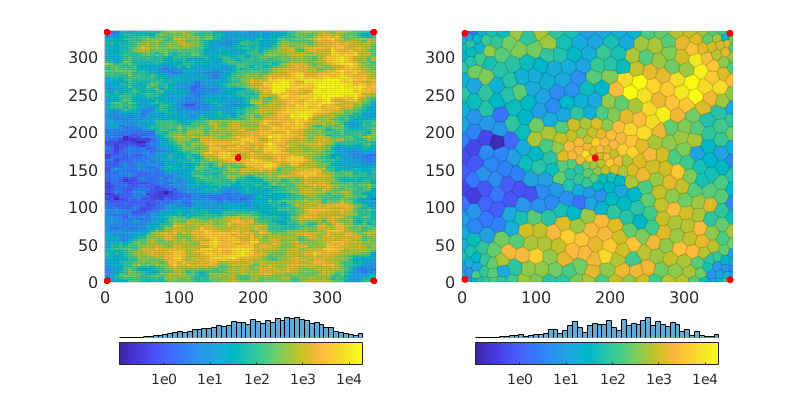
Inspect the geological model¶

figure('Position', [0,0,800,410]), subplot(1,2,1)
Kref = convertTo(rockRef.perm(:,1),milli*darcy);
plotCellData(GRef,log10(Kref),'edgeAlpha',.1); axis tight
set(gca,'FontSize',12)
mrstColorbar(Kref,'South',true); cx = caxis();
hold on; plot(xwR(:,1),xwR(:,2),'.r','MarkerSize',18); hold off

subplot(1,2,2);
K = convertTo(rock.perm(:,1),milli*darcy);
plotCellData(G,log10(K),'edgeAlpha',.1); axis tight; caxis(cx);
set(gca,'FontSize',12)
mrstColorbar(K,'South',true); axis tight
hold on; plot(xw(:,1),xw(:,2),'.r','MarkerSize',18); hold off

Set base model¶

The base model is a two-phase oil-water model

model        = GenericBlackOilModel(G, rock, fluid, 'gas', false);
pmodel       = PressureModel(model); % Pressure model
makeSeqModel = @(tmodel) ...
    SequentialPressureTransportModel(pmodel, tmodel,'parentModel', model);

Simulate with dG(0)¶

tmodelDG0 = TransportModelDG(model, 'degree', 0);
modelDG0  = makeSeqModel(tmodelDG0);
[wsDG0, stDG0, repDG0] = simulateScheduleAD(state0, modelDG0, schedule);

Getting supports.
100 of 521...
200 of 521...
300 of 521...
400 of 521...
500 of 521...
Elapsed time is 0.422063 seconds.
Inverting systems...
...

Simulate with dG(1)¶

tmodelDG1 = TransportModelDG(model, 'degree', 1);
modelDG1  = makeSeqModel(tmodelDG1);
[wsDG1, stDG1, repDG1] = simulateScheduleAD(state0, modelDG1, schedule);

Getting supports.
100 of 521...
200 of 521...
300 of 521...
400 of 521...
500 of 521...
Elapsed time is 0.377109 seconds.
Inverting systems...
...

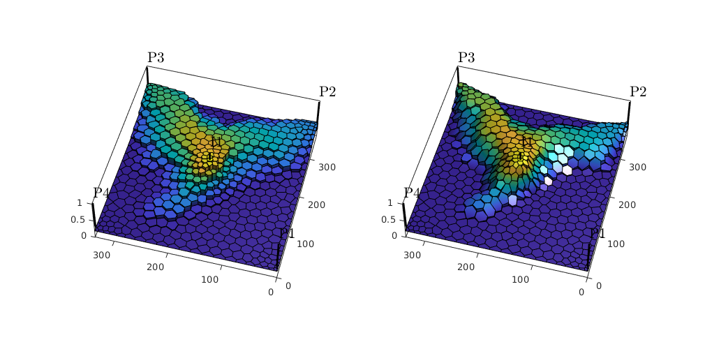
Visualize results¶

We plot the evolving saturation front computed using the two discuretizations as surface plots. To this end, we use plotSaturationDG, which supports surface plots of cell-wise discontinuous data using the patch function. Axis properties

setAxProps = @(ax) set(ax, 'Projection'        , 'Perspective', ...
                           'PlotBoxAspectRatio', [1,1,0.3]    , ...
                           'View'              , [-75,52]     , ...
                           'XLim'              , [0,l(1)]     , ...
                           'YLim'              , [0,l(2)]     , ...
                           'ZLim'              , [0,1]        , ...
                           'Box'               , 'on'         );
% For plotting wells
pw = @() plotWell(GRef, WRef, 'height', -1, 'color', 'k');
% Get coordinates for plotting (to be used in patch)
coords = getPlotCoordinates(G);
close all; figure('Position', [0,0,1000,500]);
subplot(1,2,1); % Plot dG(0)
[hs0, satDG0] = plotSaturationDG(tmodelDG0.discretization, stDG0{1}, ...
                                                         'coords', coords);
pw(); setAxProps(gca); caxis([0.2,0.8]); camlight; % Set axis properties
subplot(1,2,2); % Plot dG(1)
[h1, satDG1] = plotSaturationDG(tmodelDG1.discretization, stDG1{1}, ...
                                                         'coords', coords);
pw(); setAxProps(gca); caxis([0.2,0.8]); camlight; % Set axis properties

for i = 1:numel(stDG1)
    % Update dG(0) patch
    s0 = satDG0(stDG0{i});
    hs0.Vertices(:,3)   = s0;
    hs0.FaceVertexCData = s0;
    % Update dG(1) patch
    s1 = satDG1(stDG1{i});
    h1.Vertices(:,3)   = s1;
    h1.FaceVertexCData = s1;
    % Pause
    pause(0.2),
end

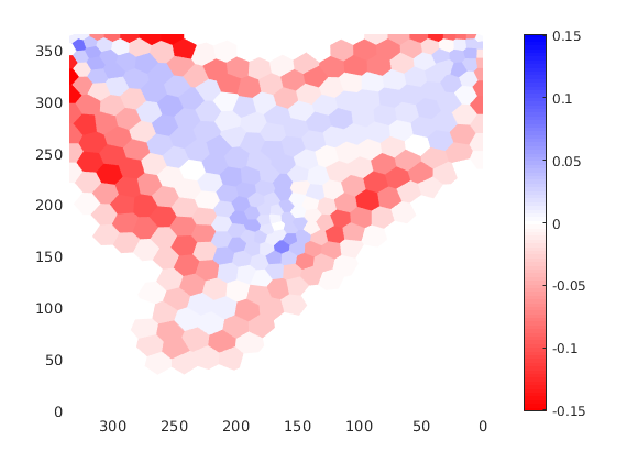
Plot the difference between the two solutions¶

figure
plotCellData(G,stDG1{end}.s(:,1)-stDG0{end}.s(:,1),'EdgeColor','none'); axis tight
view(-90,90), box on
colormap(interp1([0; 0.5; 1], [1, 0, 0; 1, 1, 1; 0, 0, 1], 0:0.01:1))
caxis([-.151 .151]);
colorbar('EastOutside');

Simulation of an inverted five-spot pattern with dG¶

Generated from dgExampleNess.m

In this example, we simulate water injection in an inverted five-spot pattern posed on a subset of SPE10 using dG(0) and dG(1) visualize the results

Add modules¶

mrstModule add dg spe10 ad-props ad-core ad-blackoil blackoil-sequential

Set up fine-scale model¶

We extract part of layer 51 of SPE10 2

[state0, imodel, schedule] = ...
    setupSPE10_AD('layers', 51, 'J',1:110,'make2D', true, 'T', 3*year, 'dt', 20*day);
G  = computeCellDimensions(imodel.G);
schedule.control.W(3).cells = 6550;
schedule.control.W(4).cells = 6578;
schedule.control.W(5).cells = 3811;

Set base model¶

model   = GenericBlackOilModel(G, imodel.rock, imodel.fluid, 'gas', false);
pmodel  = PressureModel(model); % Pressure model
tmodel0 = TransportModelDG(model, 'degree', 0);
model0  = SequentialPressureTransportModel(pmodel, tmodel0,'parentModel', model);
model0.AutoDiffBackend = DiagonalAutoDiffBackend('useMex', true);
[ws0, states0, reports0] = simulateScheduleAD(state0, model0, schedule);

Getting supports.
of 6600...
of 6600...
of 6600...
of 6600...
of 6600...
of 6600...
of 6600...
...

Simulate with dG(1)¶

tmodel1 = TransportModelDG(model, 'degree', 1, 'dsMaxAbsDiv', 2);
model1  = SequentialPressureTransportModel(pmodel, tmodel1,'parentModel', model);
model1.AutoDiffBackend = DiagonalAutoDiffBackend('useMex', true);
model1.transportNonLinearSolver = NonLinearSolver('useLinesearch', true);
[ws1, states1, reports1] = simulateScheduleAD(state0, model1, schedule);

Getting supports.
of 6600...
of 6600...
of 6600...
of 6600...
of 6600...
of 6600...
of 6600...
...

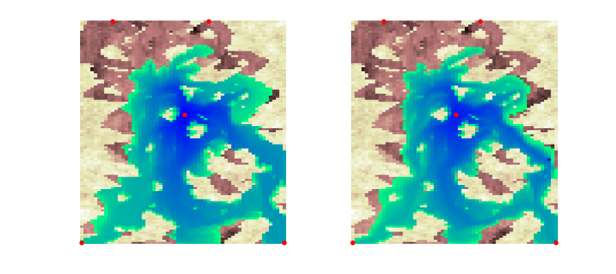
Make animation of the test case¶

To produce nice plots, we use three axes on top of each other. The first plots the permeability using a pink colormap, the second plots cells with water saturation exceeding 0.2 using a green-blue colormap, whereas the third only shows the well positions.

figure('Position', [0,0,900,400])
xw = model.G.cells.centroids(vertcat(schedule.control.W.cells),1:2);
bx1 = subplot(1,2,1);
plotCellData(G,log10(model.rock.perm(:,1)),'EdgeColor','none'); axis tight off
colormap(bx1,flipud(pink));
axlim = axis(bx1);
ax1 = axes('Position',bx1.Position);
colormap(ax1,flipud(winter));
cx1 = axes('Position',bx1.Position);
plot(xw(:,1),xw(:,2),'.r','MarkerSize',18);
axis(cx1,axlim); axis off

bx2 = subplot(1,2,2);
plotCellData(G,log10(model.rock.perm(:,1)),'EdgeColor','none'); axis tight off
colormap(bx2,flipud(pink));
ax2 = axes('Position',bx2.Position);
colormap(ax2,flipud(winter));
cx2 = axes('Position',bx2.Position);
plot(xw(:,1),xw(:,2),'.r','MarkerSize',18);
axis(cx2,axlim); axis off


[h1,h2]=deal([]);
for i=1:numel(states0)
    delete([h1 h2]);
    set(gcf,'CurrentAxes',ax1);
    h1 = plotCellData(G,states0{i}.s(:,1),states0{i}.s(:,1)>.205,'EdgeColor','none');
    axis(ax1,axlim), axis off
    set(gcf,'CurrentAxes',ax2);
    h2 = plotCellData(G,states1{i}.s(:,1),states1{i}.s(:,1)>.205,'EdgeColor','none');
    axis(ax2,axlim), axis off
    drawnow;
    pause(.2)
end

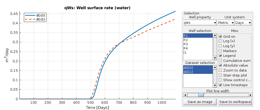
Plot production curves¶

plotWellSols({ws0, ws1},reports0.ReservoirTime,...
    'datasetnames',{'dG(0)','dG(1)'}, 'field', 'qWs');

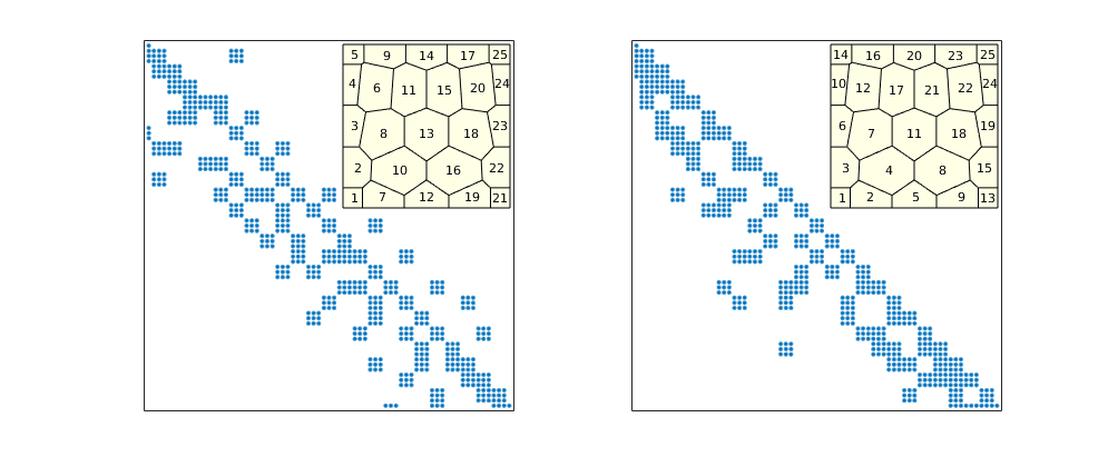
Show Sparsity Pattern¶

Generated from dgShowSparsity.m

This example compares the sparsity patterns of dG(0)/SPU and dG(1) for a small PEBI grid and shows how one can use potential ordering to permute the systems to (block)triangular form.

mrstModule add upr dg ad-core ad-props ad-blackoil blackoil-sequential

Set up the model and compute a pressure solution¶

We construct a PEBI grid using a function from the UPR module, specify a quarter five-spot type well pattern, and set up an incompressible oil-water system with unit properties and slight rock compressibility. We then split the generic black-oil model into a pressure and a transport model (with dG) and use a standalone pressure solver to compute pressure. This is used as input to compute the linearized transport equations for the dG transport solver.

G        = pebiGrid(1/4, [1,1]);
G        = computeGeometry(G);
G        = computeCellDimensions(G);
rock     = makeRock(G, 1, 1);
W        = addWell([], G, rock, 1, 'type', 'rate', 'Radius', 1e-3, ...
                    'val',  1, 'compi', [1 0], 'Name', 'I');
W        = addWell(W, G, rock, G.cells.num, 'type', 'rate', 'Radius', 1e-3,...
                    'val', -1, 'compi', [1 0], 'Name', 'P');
fluid    = initSimpleADIFluid('phases', 'WO', 'mu', [1, 1], 'rho', [1, 1], 'cR', 1e-6/barsa);
schedule = simpleSchedule(1, 'W', W);

model    = GenericBlackOilModel(G, rock, fluid, 'gas', false);
pmodel   = PressureModel(model); % Pressure model
tmodel0  = TransportModelDG(model, 'degree', 0);
model0   = SequentialPressureTransportModel(pmodel, tmodel0,'parentModel', model);

forces   = schedule.control(1);
model0   = model0.validateModel(forces);
state0   = model0.validateState(initResSol(G, 1*barsa, [0, 1]));
state    = standaloneSolveAD(state0, model0, schedule.step.val(1), 'W', forces.W);
problem  = model0.transportModel.getEquations(state0, state, 1, forces);

Getting supports.
Elapsed time is 0.067339 seconds.
Inverting systems...
Solving timestep 1/1:          -> 1 Second
*** Simulation complete. Solved 1 control steps in 3 Seconds, 17 Milliseconds ***

Sparsity pattern for dG(0)/SPU¶

Show sparsity patter before and after applying potential ordering

figure('Position',[520 360 985 420]);
subplot(1,2,1)
A0 = problem.equations{1}.jac{1};
spy(A0);
set(gca,'XTick',[],'YTick',[]); xlabel('');
axes('Position',[.31 .555 .15 .35]);
plotGrid(G,'FaceColor',[1 1 .9]);
h=text(G.cells.centroids(:,1),G.cells.centroids(:,2),num2str((1:G.cells.num)'));
set(h,'FontSize',8,'HorizontalAlignment','center','VerticalAlignment','middle')
axis off

subplot(1,2,2)
[~,q] = sort(state.pressure,'descend');
spy(A0(q,q));
set(gca,'XTick',[],'YTick',[]); xlabel('');
axes('Position',[.75 .555 .15 .35]);
plotGrid(G,'FaceColor',[1 1 .9]);
h=text(G.cells.centroids(q,1),G.cells.centroids(q,2),num2str((1:G.cells.num)'));
set(h,'FontSize',8,'HorizontalAlignment','center','VerticalAlignment','middle')
axis off

Get the discretization matrix for the dG(1) scheme¶

As for the dG(0)/SPU scheme, we first construct a transport model and a corresponding sequential model, before we compute one pressure step and use the result as input to construct the linear transport system

tmodel1  = TransportModelDG(model, 'degree', 1);
model1   = SequentialPressureTransportModel(pmodel, tmodel1,'parentModel', model);

model1   = model1.validateModel(forces);
state0   = model1.validateState(initResSol(G, 1*barsa, [0, 1]));
state    = standaloneSolveAD(state0, model1, schedule.step.val(1), 'W', forces.W);
problem  = model1.transportModel.getEquations(state0, state, 1, forces);

Getting supports.
Elapsed time is 0.048801 seconds.
Inverting systems...
Solving timestep 1/1:          -> 1 Second
*** Simulation complete. Solved 1 control steps in 3 Seconds, 648 Milliseconds ***

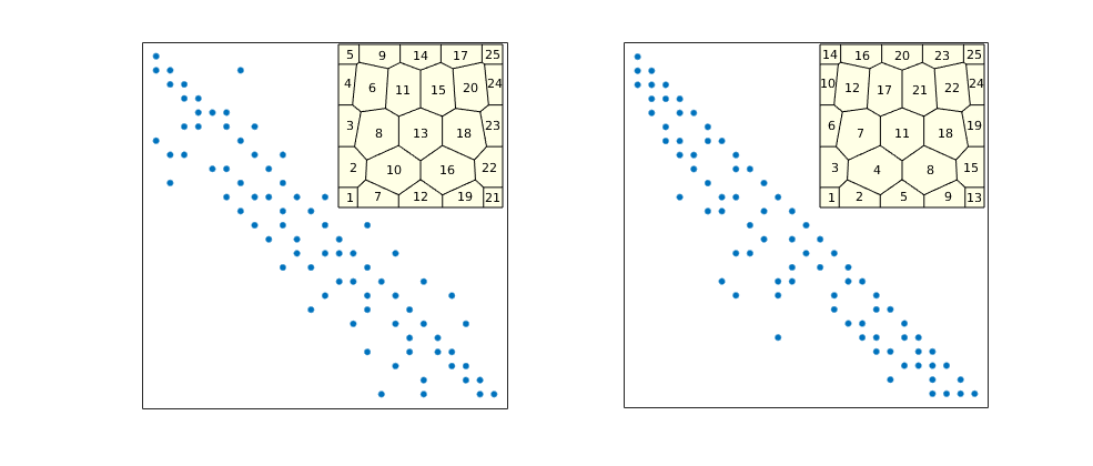
Sparsity pattern for dG(1)¶

Show the sparsity system before and after potential ordering

figure('Position',[520 360 985 420]);
subplot(1,2,1)
A1 = problem.equations{1}.jac{1};
spy(A1,8);
set(gca,'XTick',[],'YTick',[]); xlabel('');
axes('Position',[.31 .555 .15 .35]);
plotGrid(G,'FaceColor',[1 1 .9]);
h=text(G.cells.centroids(:,1),G.cells.centroids(:,2),num2str((1:G.cells.num)'));
set(h,'FontSize',8,'HorizontalAlignment','center','VerticalAlignment','middle')
axis off

subplot(1,2,2)
qq = 3*ones(G.cells.num,1); qq([1 end])=1; qq=cumsum([0; qq]);
map = cell(G.cells.num,1);
for i=1:G.cells.num
    map{i} = (qq(i)+1:qq(i+1))';
end
p=vertcat(map{q});
spy(A1(p,p),8);
set(gca,'XTick',[],'YTick',[]); xlabel('');
axes('Position',[.75 .555 .15 .35]);
plotGrid(G,'FaceColor',[1 1 .9]);
h=text(G.cells.centroids(q,1),G.cells.centroids(q,2),num2str((1:G.cells.num)'));
set(h,'FontSize',8,'HorizontalAlignment','center','VerticalAlignment','middle')
axis off

dg: Discontinous Galerkin discretizations¶

Examples¶

Buckley-Leverett displacement¶

Set up problem¶

Finite volume simulation¶

Lowest-order dG simulation¶

Simulate dG(0)¶

First-order dG simulation¶

Limiters¶

Simulate dG(1)¶

Higher-order dG simulations¶

Simulate dG(2)¶

Compare results¶

Plot dG(1) solution¶

Compare FV and dG(0) - dG(2)¶

Components of a Discontinuous Galerkin Discretization in MRST¶

Make grid¶

Plot the grid¶

Construct discretization¶

Inspect basis¶

Plot polynomial basis¶

Construct triangle cubature¶

Test the triangle cubature¶

Construct moment fitting cubature¶

Test the moment fitting cubature¶

Construct line cubature¶

Simulation of an inverted five-spot pattern with dG¶

Add modules¶

Set up fine-scale model¶

Make PEBI grid¶

Sample rock properties¶

Set up schedule and initial state¶

Inspect the geological model¶

Set base model¶

Simulate with dG(0)¶

Simulate with dG(1)¶

Visualize results¶

Plot the difference between the two solutions¶

Simulation of an inverted five-spot pattern with dG¶

Add modules¶

Set up fine-scale model¶

Set base model¶

Simulate with dG(1)¶

Make animation of the test case¶

Plot production curves¶

Show Sparsity Pattern¶

Set up the model and compute a pressure solution¶

Sparsity pattern for dG(0)/SPU¶

Get the discretization matrix for the dG(1) scheme¶

Sparsity pattern for dG(1)¶

`dg`: Discontinous Galerkin discretizations¶