vem: Virtual element method on general grids
-
Contents¶ UTILS
- Files
- addBCVEM - Add boundary condition to (new or existing) BC using function handels, computeVEMGeometry - Computes VEM geometry of MRST grid G. conserveFlux - Postprocess nonconservative flux field. polyDim - Computes the dimension of the space of polynomials of degree k or less in polygonInt - Integrates the function f over each cell in cells of grid G, using a polygonInt3D - Integrates the function f over each face in faces of 3D grid G, using a polyhedronInt - Integrates the function f over each cell in cells of grid G, using a squeezeBlockDiag - Squeezes a block diagonal matrix in which each block has the same number tetrahedronQuadRule - Returns quadrature rule for the reference terahedron with vertices V. triangleQuadRule - Returns quadrature rule for the reference triangle with vertices (0,0),
-
addBCVEM(bc, f, t, g)¶ Add boundary condition to (new or existing) BC using function handels, to be used in patch-testing and convergence tests in incompVEM.
Syntax is similar to that of addBC, but with a function handle in stead of scalar value for each boundary. Each call to addBCVEM adds a set of faces with a given type and function handle bc.
- SYNOPSIS:
- bc = addBC(bc, faces, type, function)
- PARAMETERS:
- bc - Boundary condition structure from a prior call to ‘addBCVEM’
- which will be updated on output or an empty array (bc==[]) in which case a new boundary condition structure is created.
- faces - Global faces in external model for which this boundary
- condition should be applied.
- type - Type of boundary condition. Supported values are ‘pressure’
- and ‘flux’, or cell array of such strings.
- function - Boundary condition function. Interpreted as a pressure p
(in units of ‘Pa’) when type==’pressure’ and as a -K nabla p cdot n when type==’flux’. One scalar value for each face in ‘faces’.
Note: type==’flux’ is only supported in 2D, and the function is interpreted as K nabla p cdot n.
- SEE ALSO:
- addBC
-
computeVEMGeometry(G)¶ Computes VEM geometry of MRST grid G.
- SYNOPSIS:
- G = computeVEMGeometry(G)
- DESCRIPTION:
- Computes geometry using MRST functions G = computeGeometry(G) and G = mrstGridWithFullMappings(G), and computes edge data and cell diameters. Edge data is organized in the same way as face data in 2D.
- REQUIRED PARAMETERS:
- G - MRST grid.
- RETURNS:
- G - Grid with computed VEM geometry.
See also
computeVirtualIP, incompVEM.
-
conserveFlux(state, G, rock, varargin)¶ Postprocess nonconservative flux field.
Synopsis:
[state, r] = conserveFlux(state, G, rock)
[state, r] = conserveFlux(state, G, rock, 'pn1', vn1, ...)
Description:
Postprocesses nonconsrevative flux field using a TPFA-like scheme.
Parameters: - state – Reservoir and well solution structure, result from a previous call to f.ex. function ‘incompVEM’ and, possibly, a transport solver such as function ‘explicitTransport’.
- G – Grid structure as described by grid_structure.
- rock – Rock data structure with valid field ‘perm’.
Keyword Arguments: bc – Boundary condition structure as defined by function ‘addBC’. This structure accounts for all external boundary conditions to the reservoir flow. May be empty (i.e., bc = []) which is interpreted as all external no-flow (homogeneous Neumann) conditions.
src – Explicit source contributions as defined by function ‘addSource’. May be empty (i.e., src = []) which is interpreted as a reservoir model without explicit sources.
faceWeights – The choice of face weights for the L2 norm. String. Default vale = ‘permWeighted’. Supported value are:
- permWeighted : Each face is weighted by the inverse of the sum of the inverses of the permeability in its neighbor cells.
- tpf : Face weights equals the TPFA
- tranmissibilities.
- ones : All face weights equals one.
tol – Tolerance for the residuals r_i = int Omega_i q dx - int_Omega_i v cdot n ds, If the function fails to construc a flux field with residuals norm(r)/norm(rhs) < tol, a warning is displayed. Scalar. Default value = 1e-14.
Returns: - state – Update reservoir solution structure with locally conservative fluxes.
- r – Residuals.
See also
incompVEM.
-
polyDim(k, dim)¶ Computes the dimension of the space of polynomials of degree k or less in R^dim.
- SYNOPSIS:
- polyDim(k, dim)
- REQUIRED PARAMETERS:
k - Polynomial order.
dim - Dimension of domain on which the polynomails are defined.
- RETURNS:
- nk - dimension of polynomial function space.
-
polygonInt(G, cells, f, k)¶ Integrates the function f over each cell in cells of grid G, using a quadrature rule of precision k.
- SYNOPSIS:
- I = polygonInt(G, cells, f, k)
- DESCRIPTION:
- Approximates the integrals
- int_K f dx
over specified cells K of G of using a quadrature rule of precission k. Each cell is trangulated, and a map F from reference triangle with vertices (0,0), (1,0) and (0,1) is constructed. Using that
int_K f dx = |\det(F)|int_T f(F(y)) dy,the integral can be approximated by the quadrature rule.
- REQUIRED PARAMETERS:
- G - MRST grid. cells - Cells over which to integrate f. f - Integrand. k - Precission of quadrature rule.
- RETURNS:
- I - Approximated solution to the integral.
-
polygonInt3D(G, faces, f, k)¶ Integrates the function f over each face in faces of 3D grid G, using a quadrature rule of precision k.
- SYNOPSIS:
- I = polygonInt(G, faces, f, k)
- DESCRIPTION:
Approximates the integrals
int_F f dxover specified faces F of G of using a quadrature rule of precission k. Each face is mapped from 3D to 2D, triangluated, and a map F from reference tringle Tr with vertices (0,0), (1,0) and (0,1) is constructed. Using that
int_T f dx = |\det(Fr)|int_Tr f(Fr(y)) dy,the integral can be approximated by the quadrature rule.
- REQUIRED PARAMETERS:
- G - 3D MRST grid. faces - faces over which to integrate f. k - Precision of quadrature rule.
- RETURNS:
- I - Approximated solution to the integral.
-
polyhedronInt(G, cells, f, k)¶ Integrates the function f over each cell in cells of grid G, using a quadrature rule of precision k.
- SYNOPSIS:
- I = polygonInt(G, cells, f, k)
- DESCRIPTION:
Approximates the integrals
int_K f dxover specified cells K of G of using a quadrature rule of precission k. Each cell divided into terahedra, and a map F from reference tetrahedron Tr with vertices V constructed. Using that
int_T f dx = |\det(F)|int_Tr f(F(y)) dy,the integral can be approximated by the quadrature rule.
- REQUIRED PARAMETERS:
- G - MRST grid. cells - Cells over which to integrate f. k - Precission of quadrature rule.
- RETURNS:
- I - Approximated solution to the integral.
-
squeezeBlockDiag(A, n, r, c)¶ Squeezes a block diagonal matrix in which each block has the same number of columns OR the same numer of rows.
The result is a ‘column’ or ‘row’ matrix:
[A ] [A] [A ] [ B ] -{column}-> [B] and [ B ] -{row}-> [A B C] [ C] [C] [ C]
- SYNOPSIS:
- A = squeezeBlockDiag(A, n, r, c)
- REQUIRED PARAMETERS:
- A - Block diagonal matrix in which each block has the same number
- of columns OR the same numer of rows.
n - Number of matrix blocks.
r - Number of rows in resulting matrix.
c - Number of columns in resulting matrix.
- RETURNS:
- A - Squeezed matrix.
-
tetrahedronQuadRule(k)¶ Returns quadrature rule for the reference terahedron with vertices V.
Synopsis:
[Xq, w, V, vol] = polyhedronQuadRule(k)
Description:
Returns quadrature rule of precission k, as described in [1]. Usage of the rule is as follows:
int_T f dx = volsum_{i = 1}^n w_i*f(Xq_i),where T is the reference terahedron with vertices V, f is the funtion to be integrated, vol is the area of T, and w_i and Xq_i is the ith wheight and quadrature point, respectively.
Parameters: k – Quadrature rule precision. supported values precisions are 2,3 and 7.
Returns: - Xq – nq x 3 matrix of quadrature points.
- w – nq x 1 vector of quadrature wheights.
- V – 4 x 3 matrix of reference tirangle vertices.
- vol – Area of reference triangel.
References
- [1] - http://people.sc.fsu.edu/~jburkardt/m_src/…
- tetrahedron_arbq_rule/tetrahedron_arbq_rule.html
-
triangleQuadRule(k)¶ Returns quadrature rule for the reference triangle with vertices (0,0), (1,0) and (0,1).
- SYNOPSIS:
- [Xq, w, V, vol] = triangleQuadRule(k)
- DESCRIPTION:
Returns quadrature rule of precission k. k = 1 returns the centroid rule, while k >= 2 returns rules named STRANG k, as defined in [1]. Usage of the rule is as follows:
int_T f dx = volsum_{i = 1}^n w_i*f(Xq_i),where T is the reference triangle with vertices (0,0), (1,0) and (0,1), f is the funtion to be integrated, vol is the area of T, and w_i and Xq_i is the ith wheight and quadrature point, respectively.
- REQUIRED PARAMETERS:
- k - Quadrature rule precision. supported values precisions
- are 1,2,3 and 7.
- RETURNS:
- Xq - nq x 2 matrix of quadrature points. w - nq x 1 vector of quadrature wheights. V - 3 x 2 matrix of reference tirangle vertices. vol - Area of reference triangel.
- REFERENCES:
- [1] - http://people.sc.fsu.edu/~jburkardt/datasets/…
- quadrature_rules_tri/quadrature_rules_tri.html
-
Contents¶ MRST-VEM
- Files
- computeVirtualIP - Compute local inner products for the frist- or second order virtual incompVEM - Solve incompressible flow problem (fluxes/pressures) using a first- or
-
computeVirtualIP(G, rock, k, varargin)¶ Compute local inner products for the frist- or second order virtual element method (VEM).
- SYNOPSIS:
- S = computeVirtualIP(G, rock, k) S = computeVirtualIP(G, rock, k, pn1, ‘vn1’, …)
- REQUIRED PARAMETERS:
G - Grid structure as described by grid_structure.
- rock - Rock data structure with valid field ‘perm’. The
permeability is assumed to be in measured in units of metres squared (m^2). Use function ‘darcy’ to convert from (milli)darcies to m^2, e.g.,
perm = convertFrom(perm, milli*darcy)
if the permeability is provided in units of millidarcies.
The field rock.perm may have ONE column for a scalar permeability in each cell, TWO/THREE columns for a diagonal permeability in each cell (in 2/3 D) and THREE/SIX columns for a symmetric full tensor permeability. In the latter case, each cell gets the permeability tensor
- K_i = [ k1 k2 ] in two space dimensions
- [ k2 k3 ]
- K_i = [ k1 k2 k3 ] in three space dimensions
- [ k2 k4 k5 ] [ k3 k5 k6 ]
- k - Method order. A k-th order method vil recover k-th order
- pressure fields exactly. Supported values are 1 and 2.
OPTIONAL PARAMETERS:
- innerProduct - The choice of stability term in the inner
product. String. Default value = ‘ip_simple’. Supported values are:
- ‘ip_simple’ : ‘Standard’ VEM stability term equal
- to trace(K)h^(dim-2) I.
- ‘ip_qfamily’ : Parametric family of inner products.
- ‘ip_fem’ : Inner product resembling the finite
- element mehtod on regular Cartesian grids.
- ‘ip_fd’ : Inner product resembling a
- combination of two finite difference stencils, one using the regular Cartesian coordinate axes (Fc), and one using the cell diagonals (Fd) as axes on regular Cartesian grids.
- sigma - Extra parameters to inner product
- ip_qfamily. Must be either a single scalar value, or nker values per cell, where nker is the dim of the nullspace of the projeciton operator Pi^nabla.
- w - Extra parameter to the inner product ip_fd,
- corresponding to the weighting of the two FD stencils, wFc + (1-w)Fd. Positive scalar vale.
- invertBlocks - Method by which to invert a sequence of
small matrices that arise in the discretisation. String. Supported values are:
- MATLAB : Use the MATLAB function mldivide
- (backslash) (the default).
- MEX : Use two C-accelerated MEX functions to
- extract and invert, respectively, the blocks along the diagonal of a sparse matrix. This method is often faster by a significant margin, but relies on being able to build the required MEX functions.
- trans - Fluxes can alternatively be reconstructed from the
- VEM pressure field using the TPFA or MPFA scheme. String. Supported values are ‘mpfa’ and ‘tpfa’.
- RETURNS:
- S - Pressure linear system structure having the following fields:
- A : Block diagonal matrix with the local inner products
- on the diagonal.
- order : Order k of the VEM method.
- ip : Inner product name.
- PiNstar : Block diagonal matrix with the Projection operators
- Pi^nabla in the monomial basis for each cell.
- PiNFstar: Block diagonal matrix with the Projection operators
- Pi^nabla in the monomial basis for each face of each cell. Empty if G.griddim = 2.
- faceCoords: Local 2D coordinate systems for each face if
- G.griddim = 3.
- dofVec : Map from local to global degrees of freedom.
- T, transType: If MPFA or TPFA scheme is to be used for flux
- reconstructiom, T and transType are the corresponding transmissibilites and type.
- SEE ALSO:
- incompVEM, darcy, permTensor.
-
incompVEM(state, G, S, fluid, varargin)¶ Solve incompressible flow problem (fluxes/pressures) using a first- or second-order virtual element method.
- SYNOPSIS:
- state = incompVEM(state, G, S, fluid) state = incompVEM(state, G, S, fluid, ‘pn1’, pv1, …)
- DESCRIPTION:
- This function assembles and solves a set of linear equations defining the pressure at the nodes (first order), faces, edges and cells (second order) for the reservoir simulation problem defined by Darcy’s law, sources and boundary conditions. The fluxes are reconstructed from the pressure solution.
- REQUIRED PARAMETERS:
- state - Reservoir and well solution structure either properly
- initialized from function ‘initState’, or as the results from a previous call to function ‘incompVEM’ and, possibly, a transport solver such as function ‘explicitTransport’.
- G, S - Grid and (VEM) linear system data structures as defined by
- function ‘computeVirtualIP’.
fluid - Fluid data structure as described by ‘fluid_structure’.
- OPTIONAL PARAMETERS:
- bc - Boundary condition structure as defined by function ‘addBC’.
- This structure accounts for all external boundary conditions to the reservoir flow. May be empty (i.e., bc = []) which is interpreted as all external no-flow (homogeneous Neumann) conditions. Can also be a strucutre defined by the function ‘addBCVEM’, wich allows for function handle boundary conditions for easy patch testing.
- src - Explicit source contributions as defined by function
- ‘addSource’. May be empty (i.e., src = []) which is interpreted as a reservoir model without explicit sources.
- facePressure -
- Whether or not to calculate face pressures if a first-order method is used. Defalut value: facePressure = FALSE.
- cellPressure -
- Whether or not to calculate cell pressures if a first-order method is used. Defalut value: cellPressure = FALSE.
- LinSolve -
Handle to linear system solver software to which the fully assembled system of linear equations will be passed. Assumed to support the syntax
x = LinSolve(A, b)in order to solve a system Ax=b of linear equations. Default value: LinSolve = @mldivide (backslash).
- MatrixOutput -
- Whether or not to return the final system matrix ‘A’ to the caller of function ‘incompVEM’. Logical. Default value: MatrixOutput = FALSE.
- RETURNS:
- state - Update reservoir solution structure with new values for the
- fields:
- nodePressure – Pressure values for all nodes in the
- discretized resrvoir model, ‘G’.
- edgePressure – If G.griddim = 3 and method order = 2,
- pressure values for all edges in the discretized resrvoir model, ‘G’.
- facePressure – If method order = 2 or facePressure =
- true, pressure values for all faces in the discretized resrvoir model, ‘G’.
- pressure – If method order = 2 or cellPressure =
- true, Pressure values for all cells in the discretised reservoir model, ‘G’.
- flux – If calculateFlux = true, fluxes across
- global interfaces corresponding to the rows of ‘G.faces.neighbors’.
- A – System matrix. Only returned if
- specifically requested by setting option ‘MatrixOutput’.
- SEE ALSO:
- computeVirtualIP, addBC, addBCVEM addSource, initSimpleFluid initState.
Examples
Basic VEM tutorial
Generated from vemExample1.m
In this example, we will introduce the virtual element method (VEM) solver in MRST, and show how to set up and use it to solve the single-phase pressure equation
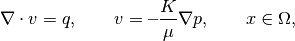
for a simple pressure drop problem. The virtual element method constitutes a unified framework for higher-order methods on general polygonal and polyhedral grids. We combine the single-phase pressure equaiton into an ellpitic equation in the pressure only;
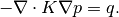
Multiplying this by a function
and integrating over
yields the weak formulation: Find
such that
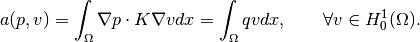
The bilinear form
can be split into a sum of local bilinear forms as
where
are the cells of the grid. For a-th order VEM, we construct approximate local bilinear forms
which are exact whevener one of
is a polynomial of degree
or less. When none of
are a such a polynomial, we only approximate
to the right order. To obtain this, we apply the following Pythagoras identity:

where
is an-orthogonal projection onto the space of polynomials of degree
or less. The approximate bilinear form is then

where
is a stability term, which we are free to choose so long as the resulting bilinear form is positive definite and stable. The flux field can easily be reconstructed from the pressure solution. For details on constructing the VEM function spaces, and implementing the method, see for example Klemetsdal 2016.
try
   require upr vem incomp vemmech
catch
   mrstModule add upr vem incomp vemmech
end
Define geometry
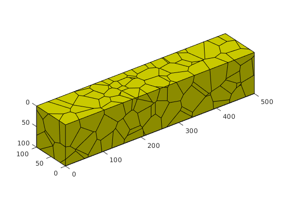
Since VEM is consistent for general polyhedral cells, we will use the UPR module to construct an arbitrary PEBI-grid. We consider a domain covering
. To generate the grid, will use the function mirroredPebi, in which we define the boundary of the domain, and the seed-points for the gridcells.
gridLimits = [500, 100, 100];

boundary  = [0             0             0             ; ...
             gridLimits(1) 0             0             ; ...
             gridLimits(1) gridLimits(2) 0             ; ...
             0             gridLimits(2) 0             ; ...
             0             0             gridLimits(3) ; ...
             gridLimits(1) 0             gridLimits(3) ; ...
             gridLimits(1) gridLimits(2) gridLimits(3) ; ...
             0             gridLimits(2) gridLimits(3)];

points = bsxfun(@times, rand(200, 3), gridLimits);

G = mirroredPebi(points, boundary);
Having generated the grid structure, we plot the result.
clf, plotGrid(G); view(3); axis equal
light('Position',[-50 -50 -100], 'Style', 'infinite')
The VEM implementation uses grid properties that are not computed by the MRST-function computeGeometry, such as cell diameters and edge normals. Thus, we compute the geometry using computeVEMGeometry. Note that this function uses computeGeometry and the function createAugmentedGrid from the VEM module for geomechanics.
G = computeVEMGeometry(G);
Define rock and fluid properties
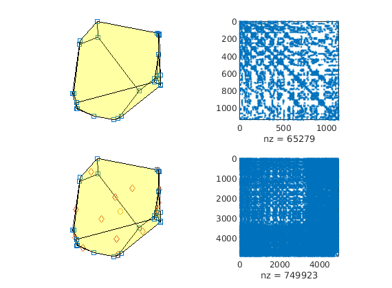
We set the permeability to be homogeneous and anisotropic,
The rock structure is constructed usin makeRock, where we let the porosity be 0.3 in all cells. The fluid is constructed using initSingleFluid. Finally, we use initResSol to initialize the state.
perm = [1000, 100, 10].* milli*darcy();
poro = 0.3;
rock = makeRock(G, perm, poro);

fluid = initSingleFluid('mu' , 100*centi*poise     , ...
                        'rho', 800*kilogram/meter^3);

state = initResSol(G, 0);
Definig boundary conditions
Since the PEBI-grid might be subject to roundoff-errors on the boundaries, we identify specific boundary faces by finding the ones that are within a given tolerance away from where we expect the boundary to be.
tol = 1e-6;

bFaces = boundaryFaces(G);
west   = abs(G.faces.centroids(bFaces,1)                ) < tol;
east   = abs(G.faces.centroids(bFaces,1) - gridLimits(1)) < tol;
We define the western and easter boundaries to be Dirichlet boundaries with a prescribed pressure. Boundaries with no prescribed boundary condition are no-flow boundaries by default.
bc = addBC([], bFaces(west), 'pressure', 500*barsa);
bc = addBC(bc, bFaces(east), 'pressure', 0        );
Constructing the linear systems
First, we compute the local inner products
. The implementation supports first and second order, and we will compute both. This is done using computeVirtualIP, where we must provide the grid and rock structures, and method order.
S1 = computeVirtualIP(G, rock, 1); disp(S1);
S2 = computeVirtualIP(G, rock, 2);
Building with 'gcc'.
Warning: You are using gcc version '7.4.0'. The version of gcc is not supported.
The version currently supported with MEX is '6.3.x'. For a list of currently
supported compilers see:
https://www.mathworks.com/support/compilers/current_release.
MEX completed successfully.
             A: [4078×4078 double]
            ip: 'ip_simple'
...
The resulting solution structure has the following fields:
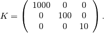
Next, we compute the solution using both first-order and second-order VEM. The first-order VEM uses the pressure at the nodes as degrees of freedom. However, it is possible to reconstruct the cell pressures of the approximated solution exactly, by uising the node pressures. This can be done by setting the optional input parameter ‘cellPressure’ to true in incompVEM. Moreover, we will invesitgate the linear system of the two methods later, so we set ‘matrixOutput’ to true.
state1 = incompVEM(state, G, S1, fluid, 'bc', bc, ...
                            'cellPressure', true, 'matrixOutput', true);
state2 = incompVEM(state, G, S2, fluid, 'bc', bc, 'matrixOutput', true);
We then plot the results.
clf

subplot(2,1,1)
plotCellData(G, state1.pressure); axis equal off; colorbar; view(3);

subplot(2,1,2)
plotCellData(G, state2.pressure); axis equal off; colorbar; view(3);
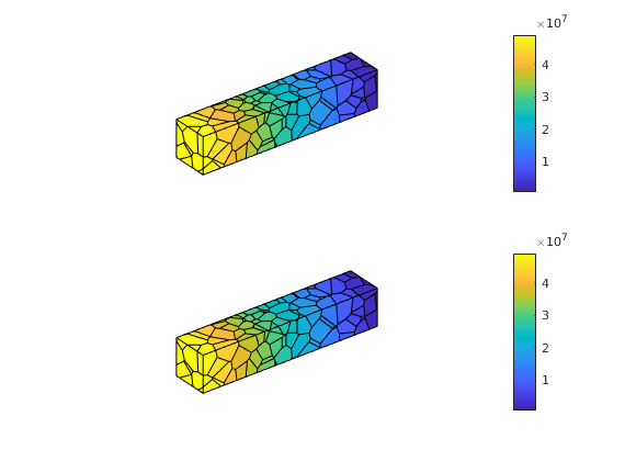
Degrees of freedom
Finally, we investigate the linear systems obtained from the two methods. We start by identifying the cell closest to the middle of the domain, its node coordinates, and face and cell centroids.
distances = sum(bsxfun(@minus, G.cells.centroids, gridLimits/2).^2,2);
midCell   = find(distances == min(distances));
midCell   = midCell(1);

n   = G.cells.nodes(G.cells.nodePos(midCell):G.cells.nodePos(midCell+1)-1);
xn  = G.nodes.coords(n,:);
f   = G.cells.faces(G.cells.facePos(midCell):G.cells.facePos(midCell+1)-1);
xf  = G.faces.centroids(f,:);
xc  = G.cells.centroids(midCell,:);
The first-order VEM uses the pressure at the nodes as degrees of freedom. The second-order VEM uses the pressure at the nodes and edge centroids, along with the average face pressure and average cell pressure. The latter yields a much denser system. We show this by indicating the degrees of freedom of the middle cell, along with a sparsity plot of the linear systems.
clf
subplot(2,2,1)
plotGrid(G, midCell, 'faceAlpha', 0.2); axis equal off;
hold on
plot3(xn(:,1), xn(:,2), xn(:,3), 'sq');

subplot(2,2,2)
spy(state1.A)

subplot(2,2,3)
plotGrid(G, midCell, 'faceAlpha', 0.2); axis equal off;
hold on
plot3(xn(:,1), xn(:,2), xn(:,3), 'sq')
plot3(xf(:,1), xf(:,2), xf(:,3), 'd')
plot3(xc(:,1), xc(:,2), xc(:,3), 'o')

subplot(2,2,4)
spy(state2.A)
The construciton of these linear systems can be quite expensive in terms of computational effort, especially for reservoir models with many cells. In order to speed up the construction, one can use C-accelerated MEX functions in computeVirtualIP. This is done by setting ‘invertBlocks’ to ‘MEX’. Note that this relies on being able to build the required MEX functions:
tic
fprintf('Computing innerproducts using mldivide \t ...
');
computeVirtualIP(G, rock, 2);
toc

tic
fprintf('Computing innerproducts using MEX \t ...
');
computeVirtualIP(G, rock, 2, 'invertBlocks', 'MEX');
toc
Computing innerproducts using mldivide         ... Elapsed time is 1.073449 seconds.
Computing innerproducts using MEX      ... Elapsed time is 0.792697 seconds.
For larger resrvoir models, using C-accelerated MEX functions is usually several orders of magnitude faster, and should always be used if possible.
Solving transport problems with VEM
Generated from vemExample2.m
In this example, we will use the virtual element method (VEM) solver in MRST, and show how to set up and use it to solve a transport problem in which we inject a high-viscosity fluid in a reservoir with varying permeability, which is initially filled with a low-viscosity fluid. To emphasize the importance of using a consistent discretization method for grids that are not K-orthogonal, we will compare the solution to the Two-point flux approximation (TPFA) mehod.
try
   require upr vem incomp vemmech
catch
   mrstModule add upr vem incomp vemmech
end
Define geometry
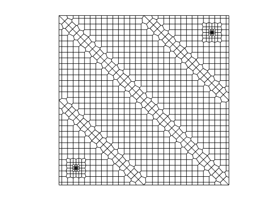
We will use the UPR module to construct a composite PEBI-grid covering the domain
, divided into three regions of highly varying permeability, with a source placed in the lower left corner, and a sink in the upper right corner. See the UPR module on how to contruct such grids.
[G, c] = producerInjectorGrid();
Having generated the grid structure, we plot the result.
clf, plotGrid(G, 'facecolor', 'none');
srcCells = find(G.cells.tag);
axis equal off
The VEM implementation uses grid properties that are not computed by the MRST-function computeGeometry, such as cell diameters and edge normals. Thus, we compute the geometry using computeVEMGeometry. Note that this function uses computeGeometry.
G = computeVEMGeometry(G);
Define rock and fluid properties
Numbering the grid regions from the lower left corner to the upper right corner, we set permeability in region
to be
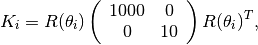
in units of 100 mD, where
is a rotation matrix
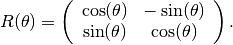
K = diag([1000, 10])*milli*darcy();
R = @(t) [cos(t) -sin(t); sin(t) cos(t)];

KK{1} = R(pi/4)*K*R(pi/4)';
KK{2} = K;
KK{3} = R(pi/2)*K*R(pi/2)';
KK{4} = K;
The structure c consists of four logical vectors identifying the cells belonging to each region, and we use this to set the permeability in each region. To define a full, symmetric permeability tensor, we specify the upper-triangular part. The rock structure is then constructed using makeRock, where we set the porosity to 0.3:
perm = zeros(G.cells.num, 3);
for i = 1:numel(c)
    perm(c{i},:) = repmat(KK{i}([1,2,4]), nnz(c{i}), 1);
end

poro = 0.3;
rock = makeRock(G, perm, poro);
We will consider a scenario in which we inject a high-viscosity fluid at a constant rate in the reservoir, which is initially filled with a fluid with lower viscosity. We define a fluid structure with these two fluids using initSimpleFluid. For simplicity, we set both phase relative permeability exponents to 1. Finally, we use initResSol to initialize the state. Here, we must indicate that the initial saturation is 0 for the fluid we are injecting, and 1 for the fluid which initially occupies the pore volume.
fluid = initSimpleFluid('mu' , [   5,    1]*centi*poise     , ...
                        'rho', [1000,  800]*kilogram/meter^3, ...
                        'n'  , [   1,    1]                      );

[stateVEM, stateTPFA] = deal(initResSol(G, 0, [0,1]));
Definig source terms
We set the injection rate equal one pore volume per 10 years. The source and sink terms are constructed using addSource. We must specify the saturation in the source term. Since want to inject fluid 1, we set this to [1,0]. We must also specify a saturation for the sink term, but this does not affect the solution.
Q   = sum(poreVolume(G,rock))/(10*year);
src = addSource([], find(G.cells.tag), [Q, -Q], 'sat', [1,0; 0,1]);
Constructing the linear systems
Next, we compute the two-point transmissibilties and virtual inner products. In this example, we use a first-order VEM.
STPFA = computeTrans(G, rock);
SVEM  = computeVirtualIP(G, rock, 1);
Warning: Matrix is close to singular or badly scaled. Results may be inaccurate.
RCOND =  1.847688e-17.
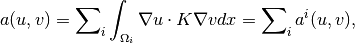
Transport
We now solve the transport problem over a time period equal to the time it takes to inject one pore volume. While TPFA is locally conservative by construction, VEM is not, which may lead to unphysical saturations when the solution is applied to the transport solver. To avoid this, we must thus postprocess the VEM solution so that the fluxes are locally conservative. This is done using conserveFlux, in which we provide any sources, sinks and boundary conditions. As for the solvers in MRST, all boundaries without prescribed boundary conditions are interpreted as no-flow boundaries. For each time step, we plot the saturation profiles and the produciton rate in the sink cell.
T  = 10*year;
nT = 100;
dT = T/nT;

[productionRateVEM, productionRateTPFA] = deal(zeros(nT,1));

t = linspace(0,T/year,nT);

for i = 1:nT

    %   Solve TPFA pressure equation.
    stateTPFA = incompTPFA(stateTPFA, G, STPFA, fluid, 'src', src);

    %   Solve TPFA transport equation.
    stateTPFA = implicitTransport(stateTPFA, G, dT, rock, fluid, 'src', src);

    %   Plot results.
    subplot(2,2,1)
    plotCellData(G, stateTPFA.s(:,1), 'edgecolor', 'none')
    caxis([0,1]);
    title('TPFA');
    axis equal off

    %   Solve VEM pressure equation.
    stateVEM = incompVEM(stateVEM, G, SVEM, fluid, 'src', src, 'cellPressure', true);

    %   Postprocess solution.
    stateVEM = conserveFlux(stateVEM, G, rock, 'src', src);

    %   Solve VEM transport equation.
    stateVEM = implicitTransport(stateVEM, G, dT, rock, fluid, 'src', src);

    %   Plot the results.
    subplot(2,2,2)
    plotCellData(G, stateVEM.s(:,1), 'edgecolor', 'none')
    caxis([0,1]);
    title('VEM');
    axis equal off

    %   Plot production in producer.
    productionRateVEM(i)  = day*Q*stateTPFA.s(src.cell(2),2);
    productionRateTPFA(i) = day*Q*stateVEM.s(src.cell(2),2);

    subplot(2,2,3:4)
    h = plot(t(1:i), productionRateVEM( 1:i), ...
             t(1:i), productionRateTPFA(1:i), 'lineWidth', 2);
    axis([0 T/year 0 1.1*day*Q])
    xlabel('Time [years]');
    ylabel('Production rate [m^3/day]');
    legend('TPFA', 'VEM')
    drawnow

end
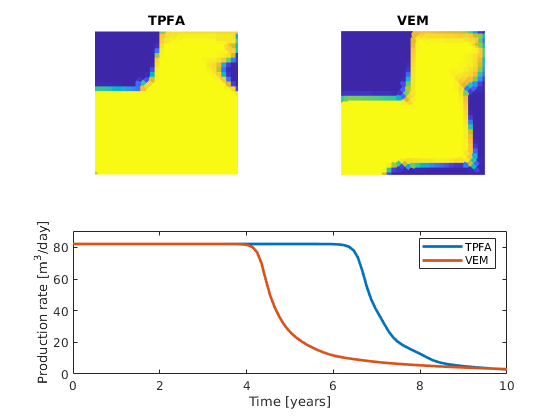
We see that there are significant differences in the two saturation profiles and production curves. This is due to the fact that TPFA fails to capture the effect of the rotated permeability fields in regions one and four.