incomp: Solvers for incompressible flow and transport
-
Contents¶ Support for incompressible flow/transport problems
- Files
- capPressureRHS - Compute capillary pressure contribution to system RHS checkDrivingForcesIncomp - Check if a solution is necessary for incompressible solvers. computeFacePressure - Compute face pressure using two-point flux approximation. computeIncompWellPressureDrop - Compute incompressible connection pressure drop for a single well computePressureRHS - Compute right-hand side contributions to pressure linear system. incompTPFA - Solve incompressible flow problem (fluxes/pressures) using TPFA method. treatLegacyForceOptions - Internal function for ensuring that both W and Wells are supported as
-
capPressureRHS(g, mob, pc, pc_form)¶ Compute capillary pressure contribution to system RHS
Synopsis:
cc = capPressureRHS(g, mob, pc, pc_form)
Description:
Calculate halfface contribution to rhs of darcy equation from the capillary pressure
g - Grid data structure.
mob - mobilities evaluated in all cells.
pc - capillary pressure evaluated in all cells, = fluid.pc(state)
pc_form - capillary pressure formulation
-
checkDrivingForcesIncomp(g, opt)¶ Check if a solution is necessary for incompressible solvers.
Synopsis:
W = addWell(W, G, rock, cellInx)
W = addWell(W, G, rock, cellInx, 'pn', pv, ...)
Parameters: - g – Valid MRST grid intended for simulation.
- opt – Merged options struct with standard incompressible options. Specifically, the forces supported by incompTPFA and incompMimetic should be included.
Returns: do_solve – Logical indicating if forces are well specified and should be solved. This check verifies that the problem is meaningful for incompressible flow.
See also
-
computeFacePressure(xr, G, T, fluid, varargin)¶ Compute face pressure using two-point flux approximation.
Synopsis:
xr = computeFacePressure(xr, G, T, fluid)
xr = computeFacePressure(xr, G, T, fluid, 'pn1', pv1, ...)
Parameters: - xr – Reservoir solution structures either properly initialized from functions ‘initResSol’ and ‘initWellSol’ respectively, or the results from a previous call to function ‘incompTPFA’ and, possibly, a transport solver such as function ‘implicitTransport’.
- T (G,) – Grid and half-transmissibilities as computed by the function ‘computeTrans’.
- fluid – Fluid object as defined by function ‘initSimpleFluid’.
Keyword Arguments: - bc – Boundary condition structure as defined by function ‘addBC’. This structure accounts for all external boundary conditions to the reservoir flow. May be empty (i.e., bc = struct([])) which is interpreted as all external no-flow (homogeneous Neumann) conditions.
- src – Explicit source contributions as defined by function ‘addSource’. May be empty (i.e., src = struct([])) which is interpreted as a reservoir model without explicit sources.
Returns: xr – Reservoir solution structure with new values for the field: - facePressure – Pressure values for all interfaces in the
discretised reservoir model, ‘G’.
See also
computeTrans,addBC,addSource,initSingleFluid,initResSol,incompTPFA.
-
computeIncompWellPressureDrop(W, mob, rho, g)¶ Compute incompressible connection pressure drop for a single well
Synopsis:
dp = computeIncompWellPressureDrop(W, mob, rho, g)
Parameters: - W – Well structure as defined by function addWell.
- mob – Phase mobilities for each cell in model.
- rho – Fluid mass densities. One scalar for each fluid phase.
- g – Norm of gravity along z-axis
Returns: dp – Column vector of size numel(W.cells). Contains each completion’s pressure drop along the well bore from the bottom hole pressure reference depth, under certain assumptions for the incompressible, linear pressure equation.
Notes
In order to avoid nonlinear behavior for wells, this function assumes that the well bore density is constant for all perforations and is equal to the injection composition if the well is an injector, either through positive rates or W.sign > 0. If the well is a producer, the mixture is assumed to be taken from the perforated cells, with flux proportional to the well indices.
See also
-
computePressureRHS(g, omega, bc, src)¶ Compute right-hand side contributions to pressure linear system.
Synopsis:
[f, g, h, grav, dF, dC] = computePressureRHS(G, omega, bc, src)
Description:
The contributions to the right-hand side for mimetic, two-point and multi-point discretisations of the equations for pressure and total velocity
v + lam K·grad (p - g·z omega) = 0 div v = q- with
- kr_i/
- lam = / / mu_i
- – i __
- omega = / f_i·rho_i
- – i
Parameters: - G – Grid data structure.
- omega – Accumulated phase densities rho_i weighted by fractional flow functions f_i – i.e., omega = sum_i rho_i f_i. One scalar value for each cell in the discretised reservoir model, G.
- bc – Boundary condition structure as defined by function ‘addBC’. This structure accounts for all external boundary conditions to the reservoir flow. May be empty (i.e., bc = struct([])) which is interpreted as all external no-flow (homogeneous Neumann) conditions.
- src – Explicit source contributions as defined by function ‘addSource’. May be empty (i.e., src = struct([])) which is interpreted as a reservoir model without explicit sources.
Returns: f, g, h – Pressure (f), source/sink (g), and flux (h) external conditions. In a problem without effects of gravity, these values may be passed directly on to linear system solvers such as ‘schurComplementSymm’.
grav –
Pressure contributions from gravity,
grav = omega·g·(x_face - x_cell)
where
omega = sum_i f_irho_i,
thus grav is a vector with one scalar value for each half-face in the model (size(G.cells.faces,1)).
dF, dC – Dirichlet/pressure condition structure. Logical array ‘dF’ is true for those faces that have prescribed pressures, while the corresponding prescribed pressure values are listed in ‘dC’. The number of elements in ‘dC’ is SUM(DOUBLE(dF)).
This structure may be used to eliminate known face pressures from the linear system before calling a system solver (e.g., ‘schurComplementSymm’).
See also
-
incompTPFA(state, G, T, fluid, varargin)¶ Solve incompressible flow problem (fluxes/pressures) using TPFA method.
Synopsis:
state = incompTPFA(state, G, T, fluid)
state = incompTPFA(state, G, T, fluid, 'pn1', pv1, ...)
Description:
This function assembles and solves a (block) system of linear equations defining interface fluxes and cell pressures at the next time step in a sequential splitting scheme for the reservoir simulation problem defined by Darcy’s law and a given set of external influences (wells, sources, and boundary conditions).
This function uses a two-point flux approximation (TPFA) method with minimal memory consumption within the constraints of operating on a fully unstructured polyhedral grid structure.
Parameters: - state – Reservoir and well solution structure either properly initialized from functions ‘initResSol’ and ‘initWellSol’ respectively, or the results from a previous call to function ‘incompTPFA’ and, possibly, a transport solver such as function ‘implicitTransport’.
- T (G,) – Grid and half-transmissibilities as computed by the function ‘computeTrans’.
- fluid – Fluid object as defined by function ‘initSimpleFluid’.
Keyword Arguments: W – Well structure as defined by function ‘addWell’. May be empty (i.e., W = []) which is interpreted as a model without any wells.
bc – Boundary condition structure as defined by function ‘addBC’. This structure accounts for all external boundary conditions to the reservoir flow. May be empty (i.e., bc = struct([])) which is interpreted as all external no-flow (homogeneous Neumann) conditions.
src – Explicit source contributions as defined by function ‘addSource’. May be empty (i.e., src = struct([])) which is interpreted as a reservoir model without explicit sources.
LinSolve – Handle to linear system solver software to which the fully assembled system of linear equations will be passed. Assumed to support the syntax
x = LinSolve(A, b)
in order to solve a system Ax=b of linear equations. Default value: LinSolve = @mldivide (backslash).
MatrixOutput – Whether or not to return the final system matrix ‘A’ to the caller of function ‘incompTPFA’. Logical. Default value: MatrixOutput = FALSE.
verbose – Enable output. Default value dependent upon global verbose settings of function ‘mrstVerbose’.
condition_number – Display estimated condition number of linear system.
gravity – The current gravity in vector form. Defaults to gravity().
Returns: state – Update reservoir and well solution structure with new values for the fields:
- pressure – Pressure values for all cells in the
discretised reservoir model, ‘G’.
- facePressure –
Pressure values for all interfaces in the discretised reservoir model, ‘G’.
- flux – Flux across global interfaces corresponding to
the rows of ‘G.faces.neighbors’.
- A – System matrix. Only returned if specifically
requested by setting option ‘MatrixOutput’.
- wellSol – Well solution structure array, one element for
each well in the model, with new values for the fields:
- flux – Perforation fluxes through all
- perforations for corresponding well. The fluxes are interpreted as injection fluxes, meaning positive values correspond to injection into reservoir while negative values mean production/extraction out of reservoir.
- pressure – Well bottom-hole pressure.
Note
If there are no external influences, i.e., if all of the structures ‘W’, ‘bc’, and ‘src’ are empty and there are no effects of gravity, then the input values ‘xr’ and ‘xw’ are returned unchanged and a warning is printed in the command window. This warning is printed with message ID
‘incompTPFA:DrivingForce:Missing’Example:
G   = computeGeometry(cartGrid([3, 3, 5]));

f   = initSingleFluid('mu' , 1*centi*poise, ...
                      'rho', 1000*kilogram/meter^3);
rock.perm = rand(G.cells.num, 1)*darcy()/100;

bc  = pside([], G, 'LEFT', 2*barsa);
src = addSource([], 1, 1);
W   = verticalWell([], G, rock, 1, G.cartDims(2), []   , ...
                   'Type', 'rate', 'Val', 1*meter^3/day, ...
                   'InnerProduct', 'ip_tpf');
W   = verticalWell(W, G, rock, G.cartDims(1), G.cartDims(2), [], ...
                   'Type', 'bhp', 'Val', 1*barsa, ...
                   'InnerProduct', 'ip_tpf');

T   = computeTrans(G, rock);

state         = initResSol (G, 10);
state.wellSol = initWellSol(G, 10);

state = incompTPFA(state, G, T, f, 'bc', bc, 'src', src, ...
                   'wells', W, 'MatrixOutput', true);

plotCellData(G, state.pressure)
See also
computeTrans,addBC,addSource,addWell,initSingleFluid,initResSol,initWellSol.
-
treatLegacyForceOptions(opt)¶ Internal function for ensuring that both W and Wells are supported as keyword arguments to incompressible solvers.
-
Contents¶ Routines for evaluating pressure and saturation dependent parameters.
- Files
- fluid_structure - Fluid structure used in MATLAB Reservoir Simulation Toolbox.
-
fluid_structure¶ Fluid structure used in MATLAB Reservoir Simulation Toolbox.
MRST’s fluid representation is a structure of function handles which compute fluid properties (e.g., density or viscosity), fluid phase saturations, and phase relative permeability curves. This representation supports generic implementation of derived quantities such as mobilities or flux functions for a wide range of fluid models.
Specifically, the ‘fluid’ structure contains the following fields:
- properties – Function handle for evaluating fluid properties such
as density or viscosity. Must support the syntaxen
mu = properties()
[mu, rho] = properties() […] = properties(state) [mu, rho, extra] = properties(state)
The first call computes the phase viscosity, the second adds phase density, and the final computes additional parameters which may be needed in complex fluid models (e.g., Black Oil).
If there are multiple PVT/property regions in the reservoir model–for instance defined by means of the ECLIPSE keyword ‘PVTNUM’–then ‘properties’ must be a cell array of function handles with one element for each property region. In this case each of the functions in ‘properties’ must support a call syntax of the form
[output] = properties(state, i)
where [output] represents one of the three output forms specified above and ‘i’ is an indicator (a LOGICAL array). The call ‘properties(state,i)’ must compute property values only for those elements where ‘i’ is TRUE.
- saturation – Function handle for evaluating fluid phase saturations.
Must support the syntaxen
s = saturation(state) s = saturation(state, extra)
The first call computes fluid phase saturations based only on the current reservoir (and well) state, while the second call may utilize additional parameters and properties–typically derived from the third syntax of function ‘properties’.
If there are multiple PVT/property regions in the reservoir model–for instance defined by means of the ECLIPSE keyword ‘PVTNUM’–then ‘saturations’ must be a cell array of function handles with one element for each property region. In this case each of the functions in ‘saturation’ must support a call syntax of the form
s = saturation(state, i) s = saturation(state, i, extra)
where ‘i’ is an indicator (a LOGICAL array). The ‘saturation’ function must compute values only for those elements where ‘i’ is TRUE.
- relperm – Function handle, or a cell array of function handles
(one element for each relative permeability region, i.e., each saturation function region) for evaluating relative permeability curves for each fluid phase. Must support the syntaxen
kr = relperm(s, state)
[kr, dkr] = relperm(s, state) [kr, dkr, d2kr] = relperm(s, state) [optional]
The first call computes the relative permeability curves at the current saturations, ‘s’. The second call additionally computes the first partial derivatives of these curves with respect to each phase saturation. Finally, the third syntax additionally computes second order derivatives. This syntax is optional and only needed in a few specific instances (e.g., when using the second order adjoint method).
See also
In case the description scrolled off screen too quickly, you may access the information at your own pace using the command
more on, help fluid_structure, more off
-
Contents¶ Files constantProperties - Construct fluid property evaluator from constant data getIncompCapillaryPressure - Undocumented Utility Function getIncompProps - Undocumented Utility Function interpRelPermTable - Fast linear interpolation of tabulated relperm function (and derivative) tabulatedSatFunc - Construct rel-perm and capillary pressure evaluators from tabulated data
-
constantProperties(mu, rho)¶ Construct fluid property evaluator from constant data
Synopsis:
properties = constantProperties(mu, rho)
Parameters: - mu – Phase viscosities in units of Pa*s.
- rho – Phase densities in units of kilogram/meter^3.
Returns: properties –
Function handle that supports the following calling convention
mu = properties()
[mu, rho] = properties()
The return values are exactly the input parameters ‘mu’ and ‘rho’ to function ‘constantProperties’, respectively.
For compatiblity with the rest of MRST, the ‘properties’ function accepts any number of input arguments. All arguments are ignored.
-
getIncompCapillaryPressure(state, fluid, varargin)¶ Undocumented Utility Function
-
getIncompProps(state, fluid)¶ Undocumented Utility Function
-
interpRelPermTable(s, kr, si)¶ Fast linear interpolation of tabulated relperm function (and derivative)
Synopsis:
 kri        = interpRelPermTable(s, kr, si)

[kri, dkri] = interpRelPermTable(s, kr, si)
Parameters: - s – Saturation nodes at which underlying function kr=kr(s) is sampled. The node values must be monotonically increasing.
- kr – Values of the underlying function kr=kr(s) at the nodes, s. Must be level or increasing.
- si – Evaluation points (saturations) for new, interpolated, relperm function values and derivatives.
Returns: kri – Column vector of piecewise linearly interpolated values of the relperm function kr=kr(s) at the evaluation points ‘si’.
dkri – Column vector of piecewise constant derivative values of the function kr=kr(s) at the evaluation points ‘si’. OPTIONAL. Only computed and returned if specifically requested.
The derivative values are defined by the piecewise formulae
‘ 0 , 0 <= si < s( 1 ), % if 0 < s(1)
- dkri = | dm, s( m ) <= si < s(m+1),
` 0 , s(end) <= si <= 1 ,
where dm = (kr(m+1) - kr(m)) / (s(m+1) - s(m)).
The caller needs to pay particular attention to the handling of sub-interval end points when computing derivatives, as the derivative is generally discontinuous.
Note
Function ‘interpRelPermTable’ is designed for efficient evaluation of tabulated relative permeability curves defined by SWOF, SGOF, SOF2 and related ECLIPSE keywords.
Using this utility function as a general interpolator is not advised.
See also
interpTable,dinterpTable,interp1q,dinterpq1.
-
tabulatedSatFunc(T)¶ Construct rel-perm and capillary pressure evaluators from tabulated data
Synopsis:
[kr, pc] = tabulatedSatFunc(table)
Parameters: table –
Tabulated data for relative permeability and capillary pressure as a function of water saturation. The table must be a three- or four-column array in which the first column is interpreted as water saturation, the second is water relative permeability and the third is relative permeability of oil. The fourth column, if present, is interpreted as the oil-water capillary pressure function, P_oil-P_wat.
The first column, saturation, must be monotonically increasing. The second column must be level or increasing, while the third column must be level or decreasing. The fourth column, if present, must be level or decreasing.
Returns: kr –
Function handle that supports the following calling convention
KR = kr(s)
[KR, dKR] = kr(s)
in which the first syntax evaluates the relative permeability function, using linear interpolation, in ‘table’ at the saturation point ‘s’ and the second syntax additionally provides derivatives of the rel-perm function (piecewise constant interpolation).
The return value ‘KR’ has one row (and two columns) for each row in the saturation ‘s’. The return value ‘dKR’, if requested, has one row and four colums for each row in the saturation ‘s’. The column values are the partial derivatives
- [ d KR(:,1) / d s(:,1) , …
d KR(:,2) / d s(:,1) , … d KR(:,1) / d s(:,2) , … d KR(:,2) / d s(:,2) ]
respectively. The diagonal of the Jacobian matrix at each saturation value may thus be extracted as ‘dKR(:, [1, 4])’.
For compatiblity with the rest of MRST, the ‘kr’ function accepts any positive number of input arguments. All arguments other than the first are ignored.
pc –
Function handle that supports the following calling convention
PC = pc(s)
[PC, dPC] = pc(s)
The return value ‘PC’ is the capillary pressure P_oil - P_wat evaluated at the saturation point ‘s’. The second return value, if requested, is the derivative of capillary pressure with respect to s(:,1).
Note
The evaluators constructed by function ‘tabulatedSatFunc’ are explicitly two-phase only. Specifically, the evaluators use only the first column of the input parameter ‘s’ and explicitly assume that the second column, if present, satisfies the saturation constraint
s(:,2) = 1 - s(:,1)
-
Contents¶ Models for various simple, incompressible fluids.
- Files
- initCoreyFluid - Initialize incompressible two-phase fluid model (res. sat., an. rel-perm). initSimpleFluid - Initialize incompressible two-phase fluid model (analytic rel-perm). initSimpleFluidJfunc - Two-phase fluid model with Leverett J-function capillary pressure initSimpleFluidPc - Initialize incompressible two-phase fluid model with capillary forces initSingleFluid - Initialize incompressible single phase fluid model.
-
initCoreyFluid(varargin)¶ Initialize incompressible two-phase fluid model (res. sat., an. rel-perm).
Synopsis:
fluid = initCoreyFluid('pn1', pv1, ...)
Parameters: 'pn'/pv – List of ‘key’/value pairs defining specific fluid characteristics. The following parameters must be defined with one value for each of the two fluid phases:
- mu – Phase viscosities in units of Pa*s.
- rho – Phase densities in units of kilogram/meter^3.
- n – Phase relative permeability exponents.
- sr – Residual phase saturation.
- kwm – Phase relative permeability at ‘sr’.
Returns: fluid – Fluid data structure as described in ‘fluid_structure’ representing the current state of the fluids within the reservoir model. Example:
fluid = initCoreyFluid('mu' , [   1,  10]*centi*poise     , ...
                       'rho', [1014, 859]*kilogram/meter^3, ...
                       'n'  , [   2,   2]                 , ...
                       'sr' , [ 0.2, 0.2]                 , ...
                       'kwm', [   1,   1]);

s = linspace(0, 1, 1001).'; kr = fluid.relperm(s);
plot(s, kr), legend('kr_1', 'kr_2')
See also
fluid_structure,initSimpleFluid,solveIncompFlow.
-
initSimpleFluid(varargin)¶ Initialize incompressible two-phase fluid model (analytic rel-perm).
Synopsis:
fluid = initSimpleFluid('pn1', pv1, ...)
Parameters: 'pn'/pv – List of ‘key’/value pairs defining specific fluid characteristics. The following parameters can be defined with one value for each of the two fluid phases:
- mu – Phase viscosities in units of Pa*s. Defaults to 1
- 1*centi*poise for each phase.
- rho – Phase densities in units of kilogram/meter^3.
- Defaults to 1.
- n – Phase relative permeability exponents.
- Defaults to 1.
Returns: fluid – Fluid data structure as described in ‘fluid_structure’ representing the current state of the fluids within the reservoir model. Example:
fluid = initSimpleFluid('mu' , [   1,  10]*centi*poise     , ...
                        'rho', [1014, 859]*kilogram/meter^3, ...
                        'n'  , [   2,   2]);

s = linspace(0, 1, 1001).'; kr = fluid.relperm(s);
plot(s, kr), legend('kr_1', 'kr_2')
See also
fluid_structure,solveIncompFlow.
-
initSimpleFluidJfunc(varargin)¶ Two-phase fluid model with Leverett J-function capillary pressure
Synopsis:
fluid = initSimpleFluidJfunc('pn1', pv1, ...)
Parameters: 'pn'/pv – List of ‘key’/value pairs defining specific fluid characteristics. The following parameters must be defined with one value for each of the two fluid phases:
- mu – Phase viscosities in units of Pa*s.
- rho – Phase densities in units of kilogram/meter^3.
- n – Phase relative permeability exponents.
- rock – Rock object containing fields ‘poro’ and ‘perm’,
- which will be used to evaluate the Leverett J-function for capillary pressure
- surf_tension – Surface tension used in the Leverett
- J-function for capillary pressure
Returns: fluid – Fluid data structure as described in ‘fluid_structure’ representing the current state of the fluids within the reservoir model. Example:
G = computeGeometry(cartGrid([40,5,1],[1000 500 1]));
state.s = G.cells.centroids(:,1)/1000;
p = G.cells.centroids(:,2)*.001;
rock = makeRock(G, p.^3.*(1e-5)^2./(0.81*72*(1-p).^2), p);
fluid = initSimpleFluidJfunc('mu' , [   1,  10]*centi*poise     , ...
       'rho', [1014, 859]*kilogram/meter^3, ...
       'n'  , [   2,   2], ...
       'surf_tension',10*barsa/sqrt(0.1/(100*milli*darcy)),...
       'rock',rock);
plot(state.s, fluid.pc(state)/barsa,'o');
See also
fluid_structure,initSimpleFluid,initSimpleFluidPc,solveIncompFlow.
-
initSimpleFluidPc(varargin)¶ Initialize incompressible two-phase fluid model with capillary forces
Synopsis:
fluid = initSimpleFluidPc('pn1', pv1, ...)
Parameters: 'pn'/pv – List of ‘key’/value pairs defining specific fluid characteristics. The following parameters must be defined with one value for each of the two fluid phases:
- mu – Phase viscosities in units of Pa*s.
- rho – Phase densities in units of kilogram/meter^3.
- n – Phase relative permeability exponents.
- pc_scale – Constant multiplying the linear capillary
- term, i.e., pc(S) = pc_scale*(1-S)
Returns: fluid – Fluid data structure as described in ‘fluid_structure’ representing the current state of the fluids within the reservoir model. Example:
fluid = initSimpleFluidPc('mu' , [   1,  10]*centi*poise     , ...
                          'rho', [1014, 859]*kilogram/meter^3, ...
                          'n'  , [   2,   2], ...
                          'pc_scale', 2*barsa);

s = linspace(0, 1, 101).'; kr = fluid.relperm(s);
subplot(1,2,1), plot(s, kr), legend('kr_1(S)', 'kr_2(S)')
x.s = [s 1-s]; pc = fluid.pc(x);
subplot(1,2,2), plot(s, pc); legend('P_c(S)');
See also
fluid_structure,initSimpleFluid,solveIncompFlow.
-
initSingleFluid(varargin)¶ Initialize incompressible single phase fluid model.
Synopsis:
fluid = initSingleFluid('pn1', pv1, ...)
Parameters: 'pn'/pv – List of ‘key’/value pairs defining specific fluid characteristics. The following parameters must be defined:
- mu – Fluid viscosity in units of Pa*s.
- rho – Fluid density in units of kilogram/meter^3.
Returns: fluid – Fluid data structure as described in ‘fluid_structure’ representing the current state of the fluid within the reservoir model. Example:
fluid = initSingleFluid('mu' ,    1*centi*poise     , ...
                        'rho', 1014*kilogram/meter^3);

s = linspace(0, 1, 1001).'; kr = fluid.relperm(s);
plot(s, kr), legend('kr')
See also
fluid_structure,initSimpleFluid,solveIncompFlow.
-
Contents¶ Routines for solving transport/saturation equation.
- Files
- explicitTransport - Explicit single-point upstream mobility-weighted transport solver for two-phase flow. implicitTransport - Implicit single-point upstream mobility-weighted transport solver for two-phase flow.
-
explicitTransport(state, G, tf, rock, fluid, varargin)¶ Explicit single-point upstream mobility-weighted transport solver for two-phase flow.
Synopsis:
state = explicitTransport(state, G, tf, rock, fluid)
state = explicitTransport(state, G, tf, rock, fluid, 'pn1', pv1, ...)
Description:
Implicit discretization of the transport equation
s_t + div[f(s)(v + mo K((rho_w-rho_o)g + grad(P_c)))] = f(s)qwhere v is the sum of the phase Darcy fluxes, f is the fractional flow function,
mw(s)- f(s) = ————-
- mw(s) + mo(s)
mi = kr_i/mu_i is the phase mobility of phase i, mu_i and rho_i are the phase viscosity and density, respectively, g the (vector) acceleration of gravity, K the permeability, and P_c(s) the capillary pressure. The source term f(s)q is a volumetric rate of water.
We use a first-order upstream mobility-weighted discretization in space and a backward Euler discretization in time. The transport equation is solved on the time interval [0,tf] by calling twophaseJacobian to build a function computing the residual of the discrete system in addition to a function taking care of the update of the solution during the time loop.
Parameters: - state – Reservoir and well solution structure either properly initialized from function ‘initState’, or the results from a previous call to function ‘solveIncompFlow’ and, possibly, a transport solver such as function ‘explicitTransport’.
- G – Grid data structure discretizing the reservoir model.
- tf – End point of time integration interval (i.e., final time). Measured in units of seconds.
- rock – Rock data structure. Must contain the field ‘rock.poro’ and, in the presence of gravity or capillary forces, valid permeabilities measured in units of m^2 in field ‘rock.perm’.
- fluid – Fluid data structure as defined in ‘fluid_structure’.
Keyword Arguments: - W – Well structure as defined by function ‘addWell’. This structure accounts for all injection and production well contribution to the reservoir flow. Default value: W = [], meaning a model without any wells.
- bc – Boundary condition structure as defined by function ‘addBC’. This structure accounts for all external boundary contributions to the reservoir flow. Default value: bc = [] meaning all external no-flow (homogeneous Neumann) conditions.
- src – Explicit source contributions as defined by function ‘addSource’. Default value: src = [] meaning no explicit sources exist in the model.
- onlygrav – Ignore content of state.flux. Default false.
- computedt – Estimate time step. Default true.
- max_dt – If ‘computedt’, limit time step. Default inf.
- dt_factor – Safety factor in time step estimate. Default 0.5.
- dt – Set time step manually. Overrides all other options.
- gravity – The current gravity in vector form. Defaults to gravity().
- satwarn – Issue a warning if saturation is more than ‘satwarn’ outside the default interval of [0,1].
Returns: state – Reservoir solution with updated saturation, state.s.
Example:
See simple2phWellExample.m
See also
twophaseJacobian,implicitTransport.
-
implicitTransport(state, G, tf, rock, fluid, varargin)¶ Implicit single-point upstream mobility-weighted transport solver for two-phase flow.
Synopsis:
state = implicitTransport(state, G, tf, rock, fluid)
state = implicitTransport(state, G, tf, rock, fluid, 'pn1', pv1, ...)
Description:
Implicit discretization of the transport equation
s_t + div[f(s)(v + mo K((rho_w-rho_o)g + grad(P_c)))] = f(s)qwhere v is the sum of the phase Darcy fluxes, f is the fractional flow function,
mw(s)- f(s) = ————-
- mw(s) + mo(s)
mi = kr_i/mu_i is the phase mobility of phase i, mu_i and rho_i are the phase viscosity and density, respectively, g the (vector) acceleration of gravity, K the permeability, and P_c(s) the capillary pressure. The source term f(s)q is a volumetric rate of water.
We use a first-order upstream mobility-weighted discretization in space and a backward Euler discretization in time. The transport equation is solved on the time interval [0,tf] by calling the private function ‘twophaseJacobian’ to build functions computing the residual and the Jacobian matrix of the discrete system in addition to a function taking care of the update of the solution during a Newton-Raphson iteration. These functions are passed to the private function ‘newtonRaphson2ph’ that implements a Newton-Raphson iteration with some logic to modify time step size in case of non-convergence.
Parameters: - state – Reservoir and well solution structure either properly initialized from function ‘initState’, or the results from a previous call to function ‘solveIncompFlow’ and, possibly, a transport solver such as function ‘implicitTransport’.
- G – Grid data structure discretizing the reservoir model.
- tf – End point of time integration interval (i.e., final time). Measured in units of seconds.
- rock – Rock data structure. Must contain the field ‘rock.poro’ and, in the presence of gravity or capillary forces, valid permeabilities measured in units of m^2 in field ‘rock.perm’.
- fluid – Fluid data structure as described by ‘fluid_structure’.
Keyword Arguments: verbose – Whether or not time integration progress should be reported to the screen. Default value: verbose = mrstVerbose.
W – Well structure as defined by function ‘addWell’. May be empty (i.e., W = []) which is interpreted as a model without any wells.
bc – Boundary condition structure as defined by function ‘addBC’. This structure accounts for all external boundary contributions to the reservoir flow. Default value: bc = [] meaning all external no-flow (homogeneous Neumann) conditions.
src – Explicit source contributions as defined by function ‘addSource’. Default value: src = [] meaning no explicit sources exist in the model.
Trans – two point flux transmissibilities. This will be used instead of rock. Useful for grids without proper geometry and or for getting consistency with pressure solver.
nltol – Absolute tolerance of iteration. The numerical solution must satisfy the condition
NORM(S-S0 + dt/porvol(out - in) - Q, INF) <= nltol
at all times in the interval [0,tf]. Default value: nltol = 1.0e-6.
lstrials – Maximum number of trials in line search method. Each new trial corresponds to halving the step size along the search direction. Default value: lstrials = 20.
maxnewt – Maximum number of inner iterations in Newton-Raphson method. Default value: maxnewt = 25.
tsref – Maximum time step refinement power. The minimum time step allowed is tf / 2^tsref. Default value: tsref = 12.
LinSolve – Handle to linear system solver software to which the fully assembled system of linear equations will be passed. Assumed to support the syntax
x = LinSolve(A, b)
in order to solve a system Ax=b of linear equations. Default value: LinSolve = @mldivide (backslash).
gravity – The current gravity in vector form. Defaults to gravity().
Returns: state – Updated reservoir/well solution object. New values for reservoir saturations, state.s.
Example:
See simple2phWellExample.
See also
explicitTransport,private/twophaseJacobian,private/newtonRaphson2ph.
Examples
Norne: Single-Phase Pressure Solver
Generated from incompExampleNorne1ph.m
In the example, we will solve the single-phase pressure equation
using the corner-point geometry from the Norne field. The purpose of this example is to demonstrate how the two-point flow solver can be applied to compute flow on a real grid model that has degenerate cell geometries and non-neighbouring connections arising from a large number of faults, eroded layers, pinch-outs, and inactive cells. A more thorough examination of the model is given in a the Norne overview.
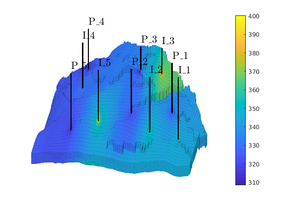
We will not use real data for rock parameters and well paths. Instead, synthetic permeability data are generated by (make-believe) geostatistics and vertical wells are placed quite haphazardly throughout the domain. Experimentation with this model is continued in incompNorne2ph.m, in which we solve a simplified two-phase model.
mrstModule add incomp
Read and process the model
Before running this example, you should run the showNorne tutorial. We start by reading the model from a file in the Eclipse formate (GRDECL). As shown in this overview, the model has two components, of which we will only use the first one.
grdecl = fullfile(getDatasetPath('norne'), 'NORNE.GRDECL');
grdecl = readGRDECL(grdecl);
usys   = getUnitSystem('METRIC');
grdecl = convertInputUnits(grdecl, usys);
G = processGRDECL(grdecl); clear grdecl;
G = computeGeometry(G(1));
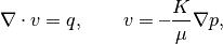
Set rock and fluid data
The permeability is lognormal and isotropic within nine distinct layers and is generated using our simplified ‘geostatistics’ function and then transformed to lay in the interval 200-2000 mD. The single fluid has density 1000 kg/m^3 and viscosity 1 cP.
gravity off
K          = logNormLayers(G.cartDims, rand(9,1), 'sigma', 1.5);
K          = 200 + (K-min(K))/(max(K)-min(K))*1800;
perm       = convertFrom(K(G.cells.indexMap), milli*darcy); clear K;
rock       = makeRock(G, perm, 1);
fluid      = initSingleFluid('mu' ,    1*centi*poise     , ...
                             'rho', 1000*kilogram/meter^3);

clf,
K = log10(rock.perm);
plotCellData(G,K,'EdgeColor','k','EdgeAlpha',.1);
axis tight off, view(15,60),
cs = [200 400 700 1000 1500 2000];
caxis(log10([min(cs) max(cs)]*milli*darcy));
h=colorbarHist(K,caxis,'South',100);
set(h, 'XTick', log10(cs*milli*darcy), 'XTickLabel', num2str(round(cs)'));
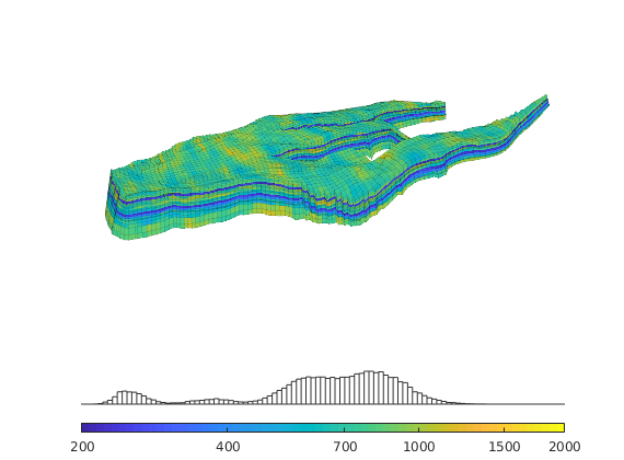
Introduce wells
The reservoir is produced using a set production wells controlled by bottom-hole pressure and rate-controlled injectors. Wells are described using a Peacemann model, giving an extra set of equations that need to be assembled. For simplicity, all wells are assumed to be vertical and are assigned using the logical (i,j) subindex.
% Plot grid outline
clf
subplot('position',[0.02 0.02 0.96 0.96]);
plotGrid(G,'FaceColor','none','EdgeAlpha',0.1);
axis tight off, view(-5,58)

% Set six vertical injectors, completed in each layer.
nz = G.cartDims(3);
I = [ 9, 26,  8, 25, 35,  10];
J = [14, 14, 35, 35, 68,  75];
R = [ 2,  2,  4,  4, 0.5,0.5]*1000*meter^3/day;
radius = .1; W = [];
for i = 1 : numel(I),
   W = verticalWell(W, G, rock, I(i), J(i), 1:nz, 'Type', 'rate', ...
                    'InnerProduct', 'ip_tpf', ...
                    'Val', R(i), 'Radius', radius, 'Comp_i', 1, ...
                    'name', ['I$_{', int2str(i), '}$']);
end
plotGrid(G, vertcat(W.cells), 'FaceColor', 'b');
prod_off = numel(W);

% Set five vertical producers, completed in each layer.
I = [17, 12, 25, 35, 15];
J = [23, 51, 51, 88, 94];
for i = 1 : numel(I),
   W = verticalWell(W, G, rock, I(i), J(i), 1:nz, 'Type', 'bhp', ...
                    'InnerProduct', 'ip_tpf', ...
                    'Val', 300*barsa(), 'Radius', radius, ...
                    'name', ['P$_{', int2str(i), '}$'], 'Comp_i', 0);
end
plotGrid(G, vertcat(W(prod_off + 1 : end).cells), 'FaceColor', 'r');
plotWell(G,W,'height',200);
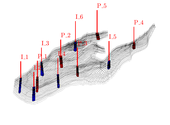
Compute transmissibilities and solve linear system
First, we compute one-sided transmissibilities for each local face of each cell in the grid. Then, we form a two-point discretization by harmonic averaging the one-sided transmissibilities and solve the resulting linear system to obtain pressures and fluxes.
T    = computeTrans(G, rock);
rSol = initState(G, W, 350*barsa, 1);
rSol = incompTPFA(rSol, G, T, fluid, 'wells', W);
Plot the fluxes
clf
cellNo  = rldecode(1:G.cells.num, diff(G.cells.facePos), 2) .';
plotCellData(G, sqrt(accumarray(cellNo,  ...
   abs(convertTo(faceFlux2cellFlux(G, rSol.flux), meter^3/day)))), ...
   'EdgeColor', 'k','EdgeAlpha',.1);
plotWell(G,W,'height',200,'color','c');
h=colorbar('horiz'); axis tight off; view(20,80)
camdolly(0,.15,0);
set(h,'Position',get(h,'Position')+[.18 -.08 -.1 0]);
Plot the pressure distribution
clf
plotCellData(G, convertTo(rSol.pressure(1:G.cells.num), barsa), ...
             'EdgeColor','k','EdgeAlpha',.1);
plotWell(G, W, 'height', 200, 'color', 'b');
h=colorbar('horiz'); axis tight off; view(20,80)
camdolly(0,.15,0);
set(h,'Position',get(h,'Position')+[.18 -.08 -.1 0]);
<html>
% <p><font size="-1
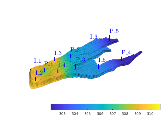
SAIGUP: Solving One-Phase Flow on a Realistic Corner-Point Model
Generated from incompExampleSAIGUP1ph.m
In the example, we will solve the single-phase pressure equation
using the corner-point geometry from synthetic reservoir model from the SAIGUP study. The purpose of this example is to demonstrate how the two-point flow solver can be applied to compute flow on a real grid model that has degenerate cell geometries and non-neighbouring connections arising from a number of faults, and inactive cells. A more thorough examination of the model is given in a showSAIGUP example. Experimentation with this model is continued in incompSAIGUP2ph.m, in which we solve a simplified two-phase model.
mrstModule add incomp
Read model data and convert units
The model data is provided as an ECLIPSE input file that can be read using the readGRDECL function.
grdecl = fullfile(getDatasetPath('SAIGUP'), 'SAIGUP.GRDECL');
grdecl = readGRDECL(grdecl);
MRST uses the strict SI conventions in all of its internal calculations. The SAIGUP model, however, is provided using the ECLIPSE ‘METRIC’ conventions (permeabilities in mD and so on). We use the functions getUnitSystem and convertInputUnits to assist in converting the input data to MRST’s internal unit conventions.
usys   = getUnitSystem('METRIC');
grdecl = convertInputUnits(grdecl, usys);
Define geometry and rock properties
We generate a space-filling geometry using the processGRDECL function and then compute a few geometric primitives (cell volumes, centroids, etc.) by means of the computeGeometry function.
G = processGRDECL(grdecl);
G = computeGeometry(G);
The media (rock) properties can be extracted by means of the grdecl2Rock function.
rock = grdecl2Rock(grdecl, G.cells.indexMap);
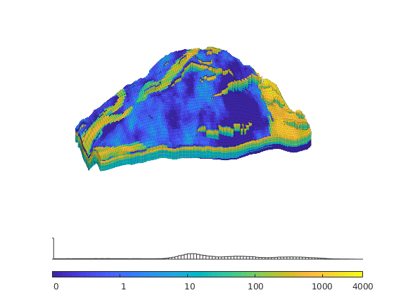
Modify the permeability to avoid singular tensors
The input data of the permeability in the SAIGUP realisation is an anisotropic tensor with zero vertical permeability in a number of cells. We work around this issue by (arbitrarily) assigning the minimum positive vertical (cross-layer) permeability to the grid blocks that have zero cross-layer permeability.
is_pos                = rock.perm(:, 3) > 0;
rock.perm(~is_pos, 3) = min(rock.perm(is_pos, 3));
Plot the logarithm of the permeability in the x-direction
clf,
K = log10(rock.perm(:,1));
plotCellData(G,K,'EdgeColor','k','EdgeAlpha',0.1);
set(gca,'dataasp',[15 15 2]);
axis off, view(-110,18);
cs = [0.1 1 10 100 1000 4000];
caxis(log10([min(cs) max(cs)]*milli*darcy));
h=colorbarHist(K,caxis,'South',100); camdolly(.2, 0, 0);
set(h, 'XTick', log10(cs*milli*darcy), 'XTickLabel', num2str(round(cs)'));
Set fluid data
The single fluid has density 1000 kg/m^3 and viscosity 1 cP.
gravity off
fluid      = initSingleFluid('mu' ,    1*centi*poise     , ...
                             'rho', 1000*kilogram/meter^3);
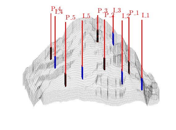
Introduce wells
The reservoir is produced using a set of production wells controlled by bottom-hole pressure and rate-controlled injectors. Wells are described using a Peacemann model, giving an extra set of equations that need to be assembled. For simplicity, all wells are assumed to be vertical and are assigned using the logical (i,j) subindex.
% Plot grid outline
clf
plotGrid(G,'FaceColor','none','EdgeAlpha',0.1);
axis tight off, view(-100,8)

% Set six vertical injectors, completed in each layer.
nz = G.cartDims(3);
I = [ 9,  8, 25, 25, 10];
J = [14, 35, 35, 95, 75];
R = [ 2,  4,  4, 1,5]*500*meter^3/day;
radius = .1; W = [];
for i = 1 : numel(I),
   W = verticalWell(W, G, rock, I(i), J(i), 1:nz, 'Type', 'rate', ...
                    'InnerProduct', 'ip_tpf', ...
                    'Val', R(i), 'Radius', radius, 'Comp_i', 1, ...
                    'name', ['I$_{', int2str(i), '}$']);
end
plotGrid(G, vertcat(W.cells), 'FaceColor', 'b','EdgeAlpha',0.1);
prod_off = numel(W);

% Set five vertical producers, completed in each layer.
I = [17, 12, 25, 33, 7];
J = [23, 51, 51, 95, 94];
for i = 1 : numel(I),
   W = verticalWell(W, G, rock, I(i), J(i), 1:nz, 'Type', 'bhp', ...
                    'InnerProduct', 'ip_tpf', ...
                    'Val', 300*barsa(), 'Radius', radius, ...
                    'name', ['P$_{', int2str(i), '}$'], 'Comp_i', 0);
end
plotGrid(G, vertcat(W(prod_off + 1 : end).cells), 'FaceColor', 'r');
plotWell(G,W,'height',30);
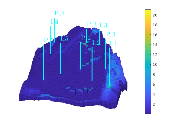
Compute transmissibilities and solve linear system
First, we compute one-sided transmissibilities for each local face of each cell in the grid. Then, we form a two-point discretization by harmonic averaging the one-sided transmissibilities and solve the resulting linear system to obtain pressures and fluxes.
T    = computeTrans(G, rock);
rSol = initState(G, W, 350*barsa, 1);
rSol = incompTPFA(rSol, G, T, fluid, 'wells', W);
Plot the fluxes
clf
cellNo  = rldecode(1:G.cells.num, diff(G.cells.facePos), 2) .';
plotCellData(G, sqrt(accumarray(cellNo,  ...
   abs(convertTo(faceFlux2cellFlux(G, rSol.flux), meter^3/day)))), ...
   'EdgeColor', 'k','EdgeAlpha',0.1);
plotWell(G,W,'height',100,'color','c');
colorbar, axis tight off; view(-80,36)
Plot the pressure distribution
clf
plotCellData(G, convertTo(rSol.pressure(1:G.cells.num), barsa), ...
   'EdgeColor','k','EdgeAlpha',0.1);
plotWell(G, W, 'height', 100, 'color', 'k');
colorbar, axis tight off; view(-80,36)
<html>
% <p><font size="-1
Basic Flow-Solver Tutorial
Generated from incompIntro.m
The purpose of this example is to give an overview of how to set up and use a standard two-point pressure solver to solve the single-phase pressure equation
for a flow driven by Dirichlet and Neumann boundary conditions. Our geological model will be simple a Cartesian grid with anisotropic, homogeneous permeability. In this tutorial example, you will learn about:
mrstModule add incomp
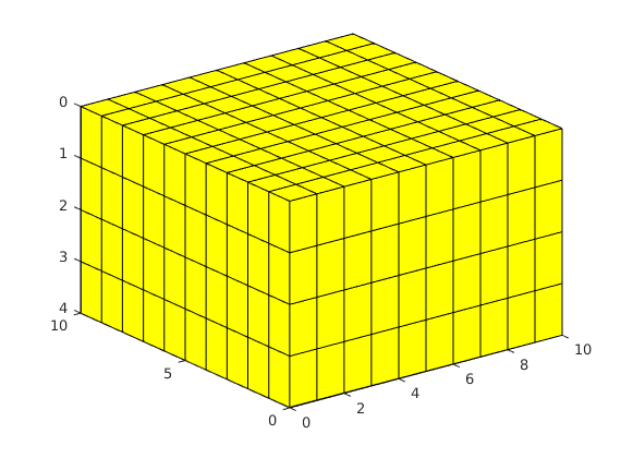
Define geometry
Construct a Cartesian grid of size 10-by-10-by-4 cells, where each cell has dimension 1-by-1-by-1. Because our flow solvers are applicable for general unstructured grids, the Cartesian grid is here represented using an unstructured format, in which cells, faces, nodes, etc. are given explicitly.
nx = 10; ny = 10; nz = 4;
G = cartGrid([nx, ny, nz]);
display(G);
G =

  struct with fields:

       cells: [1×1 struct]
       faces: [1×1 struct]
       nodes: [1×1 struct]
...
After the grid structure is generated, we plot the geometry.
clf, plotGrid(G); view(3)
Process geometry
Having set up the basic structure, we continue to compute centroids and volumes of the cells and centroids, normals, and areas for the faces. For a Cartesian grid, this information can trivially be computed, but is given explicitly so that the flow solver is compatible with fully unstructured grids.
G = computeGeometry(G);
Set rock and fluid data
The only parameters in the single-phase pressure equation are the permeability
and the fluid viscosity. We set the permeability to be homogeneous and anisotropic
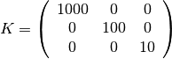
The viscosity is specified by saying that the reservoir is filled with a single fluid, for which de default viscosity value equals unity. Our flow solver is written for a general incompressible flow and requires the evaluation of a total mobility, which is provided by the fluid object.
gravity off
rock = makeRock(G, [1000, 100, 10].* milli*darcy(), 1);
fluid     = initSingleFluid('mu' ,    1*centi*poise     , ...
                            'rho', 1014*kilogram/meter^3);
Initialize reservoir simulator
To simplify communication among different flow and transport solvers, all unknowns are collected in a structure. Here this structure is initialized with uniform initial reservoir pressure equal 0 and (single-phase) saturation equal 0.0 (using the default behavior of initResSol)
resSol = initResSol(G, 0.0);
display(resSol);
resSol =

  struct with fields:

    pressure: [400×1 double]
        flux: [1380×1 double]
           s: [400×1 double]
Impose Dirichlet boundary conditions
Our flow solvers automatically assume no-flow conditions on all outer (and inner) boundaries; other type of boundary conditions need to be specified explicitly. Here, we impose Neumann conditions (flux of 1 m^3/day) on the global left-hand side. The fluxes must be given in units of m^3/s, and thus we need to divide by the number of seconds in a day (day()). Similarly, we set Dirichlet boundary conditions p = 0 on the global right-hand side of the grid, respectively. For a single-phase flow, we need not specify the saturation at inflow boundaries. Similarly, fluid composition over outflow faces (here, right) is ignored by pside.
bc = fluxside([], G, 'LEFT',  1*meter^3/day());
bc = pside   (bc, G, 'RIGHT', 0);
display(bc);
bc =

  struct with fields:

     face: [80×1 double]
     type: {1×80 cell}
    value: [80×1 double]
...
Construct linear system
Compute transmissibilities based on input grid and rock properties and use this to set up the linear system.
T = computeTrans(G, rock, 'Verbose', true);

% Solve linear system construced from T and bc to obtain solution for flow
% and pressure in the reservoir. The <matlab:help('incompTPFA')
% option> 'MatrixOutput=true' adds the system matrix A to resSol to enable
% inspection of the matrix.
resSol = incompTPFA(resSol, G, T, fluid, ...
                   'bc', bc, 'MatrixOutput', true);
display(resSol);
Computing one-sided transmissibilities...     Elapsed time is 0.001160 seconds.

resSol =

  struct with fields:

        pressure: [400×1 double]
            flux: [1380×1 double]
...
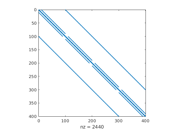
Inspect results
The resSol object contains the matrix used to solve the system.
spy(resSol.A);
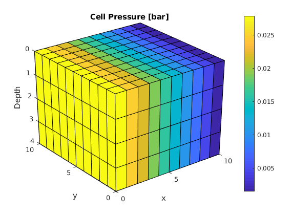
- We then plot convert the computed pressure to unit
- ‘bar’ before plotting result.
clf
plotCellData(G, convertTo(resSol.pressure(1:G.cells.num), barsa()), ...
             'EdgeColor', 'k');
title('Cell Pressure [bar]')
xlabel('x'), ylabel('y'), zlabel('Depth');
view(3); shading faceted; camproj perspective; axis tight;
colorbar
Copyright notice
<html>
% <p><font size="-1
Pressure Solver: Simple Corner-Point Grid with Linear Pressure Drop
Generated from incompTutorialCornerPoint.m
Herein we will solve the single-phase pressure equation
for a simple corner-point grid model with isotropic, lognormal permeability. The purpose of this example is to demonstrate the two-point pressure solver applied to a case with corner-point grids given as from an input stream in the industry-standard Eclipse™ format.
mrstModule add incomp
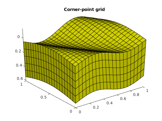
Generate the corner-point grid
The corner-point grid is generated using a standard MATLAB® meshgrid which is then transformed to make sloping pillars and wavy layers. The corner-point grid is represented as a GRDECL structure, which is the same structure as is returned from readGRDECL. If an extra parameter is passed to the simpleGrdecl function, it adds a fault to the model.
nc = [20, 20, 5];
grdecl = simpleGrdecl(nc);        % No fault in model
Then we process the GRDECL structure and build up an unstructured grid.
G = processGRDECL(grdecl); clear grdecl
After the grid structure is generated, we plot the geometry.
clf, plotGrid(G);
title('Corner-point grid')
view(3), camproj perspective, axis tight, camlight headlight
Compute geometry information
Having set up the basic structure, we continue to compute centroids and volumes of the cells and centroids, normals, and areas for the faces.
G = computeGeometry(G, 'Verbose', true);
Processing Cells    1 : 2000 of 2000 ... done (0.02 [s], 1.01e+05 cells/second)
Total 3D Geometry Processing Time = 0.021 [s]
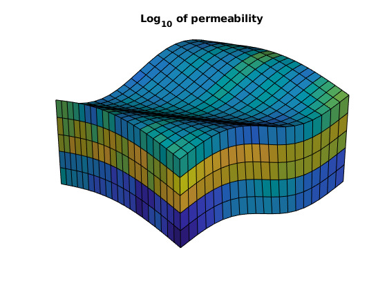
Make rock and fluid data
We generate a lognormal and layered permeability and specify that we are working with a single-phase fluid; type “help initSingleFluid” to see default values for density and viscosity. Our flow solver is constructed for a general incompressible flow and thus requires the evaluation of a total mobility function, which in our case equals one in the whole domain.
perm = convertFrom(logNormLayers(nc, [100, 400, 50]), milli*darcy());
rock = makeRock(G, perm, 1);
fluid     = initSingleFluid('mu' ,    1*centi*poise     , ...
                            'rho', 1014*kilogram/meter^3);
Plot the logarithm of the layered permeability.
cla,
plotCellData(G, log10(rock.perm(:)));
title('Log_{10} of permeability')
camproj perspective, axis tight off, camlight headlight
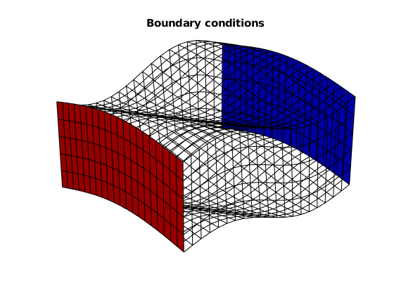
Add boundary conditions
Pressure is set of one bar on the west-side boundary and zero on the east-side boundary. No-flow conditions are imposed automatically at all other (outer) boundaries.
westFaces = find(G.faces.centroids(:,1) == 0);
bc = addBC([], westFaces, 'pressure',        ...
           repmat(1*barsa(), [numel(westFaces), 1]));

xMax = max(G.faces.centroids(:,1));
eastFaces = find(G.faces.centroids(:,1) == xMax);
bc = addBC(bc, eastFaces, 'pressure',        ...
           zeros(numel(eastFaces), 1));
Then we plot the grid, coloring the faces on which we have imposed boundary conditions.
cla,
plotGrid(G, 'FaceColor', 'none');
plotFaces(G, westFaces, 'r');
plotFaces(G, eastFaces, 'b');
title('Boundary conditions')
camproj perspective, axis tight off, camlight headlight
Assemble and solve system
Finally, we compute transmissibilities, construct two-point discretization and solve the corresponding linear equations.
rSol = initResSol(G, 0);
T    = computeTrans(G, rock, 'Verbose', true);
rSol = incompTPFA(rSol, G, T, fluid, 'MatrixOutput', true, 'bc', bc);
Computing one-sided transmissibilities... Elapsed time is 0.003085 seconds.
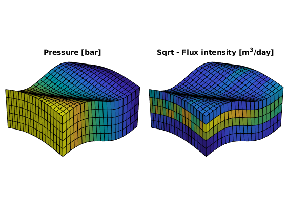
We plot the results: cell pressure is converted to unit ‘bar’ and fluxes to unit m^3/day when plotting results.
subplot('Position',[0.01 0.25 0.48 0.5]),
   plotCellData(G, convertTo(rSol.pressure(1:G.cells.num), barsa()));
   title('Pressure [bar]')
   view(3), camproj perspective, axis tight off, camlight headlight

subplot('Position',[0.51 0.25 0.48 0.5]),
   cellNo  = rldecode(1:G.cells.num, diff(G.cells.facePos), 2) .';
   plotCellData(G, sqrt(accumarray(cellNo, ...
      abs(convertTo(faceFlux2cellFlux(G, rSol.flux), meter^3/day)))));
   title('Sqrt - Flux intensity [m^3/day]')
   view(3), camproj perspective, axis tight off, camlight headlight
Copyright notice
<html>
% <p><font size="-1
How to Specify Sources and Boundary Conditions
Generated from incompTutorialSRCandBC.m
This example shows how to set up a combination of source and boundary conditions and is a continuation of the introduction to the incompressible solvers in MRST.
mrstModule add incomp
Define grid, rock and fluid data
Construct a Cartesian grid of size nx-by-ny-by-nz cells, where each cell has dimension 1-by-1-by-1 m. Set an isotropic and homogeneous permeability of 100 mD, a fluid viscosity of 1 cP and a fluid density of 1000 kg/m^3.
nx = 20; ny = 20; nz = 10;
G = cartGrid([nx, ny, nz]);
G = computeGeometry(G);
rock = makeRock(G, 100*milli*darcy, 1);
fluid     = initSingleFluid('mu' ,    1*centi*poise     , ...
                            'rho', 1014*kilogram/meter^3);
gravity reset on
Add sources and boundary conditions
The simplest way to model inflow or outflow from the reservoir is to use a fluid source/sink. Here we specify a source with flux rate of 1m^3/day in each grid cell.
c   = (nx/2*ny+nx/2 : nx*ny : nx*ny*nz) .';
src = addSource([], c, ones(size(c)) ./ day());
display(src);
src =

  struct with fields:

    cell: [10×1 double]
    rate: [10×1 double]
     sat: []
Our flow solvers automatically assume no-flow conditions on all outer (and inner) boundaries; other types of boundary conditions need to be specified explicitly. Here we impose a Dirichlet boundary condition of p=10 bar at the global left-hand side of the model. For a single-phase flow, we do not need to specify fluid saturation at the boundary and the last argument is therefor left empty.
bc = pside([], G, 'LEFT', 10*barsa());
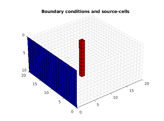
To check that boundary conditions and sources are placed at the correct location, we plot the model.
subplot(2,2,1), pos = get(gca,'Position'); clf
plotGrid(G,    'FaceColor', 'none', 'EdgeAlpha',.1);
plotGrid(G, c, 'FaceColor', 'r');
plotFaces(G, bc.face, 'b');
title('Boundary conditions and source-cells')
view(3), camproj perspective, axis tight equal, camlight headlight
h = gca;
Construct and solve the linear system
Compute transmissibilities based on input grid and rock properties and use this to set up the linear system.
T = computeTrans(G, rock, 'Verbose', true);
Computing one-sided transmissibilities... Elapsed time is 0.003898 seconds.
Compute the solution for the system with sources and boundary conditions
rSol = initResSol(G, 0);
rSol = incompTPFA(rSol, G, T, fluid, 'MatrixOutput', true, ...
                  'src', src, 'bc', bc);
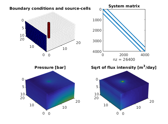
Plot output
We convert the cell pressure to unit bar and the fluxes to unit m^3/day when plotting the results. Although it is not strictly necessary here, we show how to make shorthands to simplify the plotting.
cellNo    = rldecode(1:G.cells.num, diff(G.cells.facePos), 2) .';
plot_var  = @(x) plotCellData(G, x, 'EdgeColor','none');
plot_pres = @(x) plot_var(convertTo(x.pressure(1:G.cells.num), barsa()));
plot_flux = @(x) plot_var(accumarray(cellNo, ...
   abs(convertTo(faceFlux2cellFlux(G, x.flux), meter^3/day))));

set(h,'Position',pos); % move first plot to subplot(2,2,1);

subplot(2,2,2)
spy(rSol.A)
title('System matrix')

subplot(2,2,3)
plot_pres(rSol);
title('Pressure [bar]')
view(3), camproj perspective, axis tight equal, camlight headlight

subplot(2,2,4)
plot_flux(rSol);
title('Sqrt of flux intensity [m^3/day]')
view(3), camproj perspective, axis tight equal, camlight headlight
Copyright notice
<html>
% <p><font size="-1
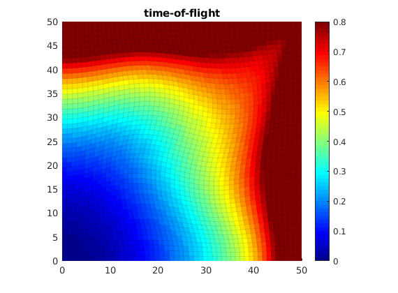
Time-of-flight
Generated from incompTutorialTOF.m
To study how heterogeneity affects flow patterns and define natural time-lines in the reservoir, it is common to study the so-called time-of-flight (TOF), i.e., the time it takes an imaginary particle released at an inflow boundary or at a perforation of an injector to reach a given point in the reservoir. Time-of-flight are usually associated with streamline methods, but can also be computed from linear steady-state transport equations on the form,

In this example, we will show how to compute time-of-flight from a given flux field.
mrstModule add incomp diagnostics
Setup model
As our model, we will use a logically Cartesian grid in which the node perturbed so that grid lines form curves and not lines. For simplicity, we assume unit permeability and porosity and use a set of source and sink terms to emulate a quater five-point setup.
G = cartGrid([50,50]);
G = twister(G);
G = computeGeometry(G);
rock = makeRock(G, 1, 1);
fluid = initSimpleFluid('mu' , [ 1, 10]*centi*poise , ...
'rho', [1014, 859]*kilogram/meter^3, ...
'n' , [ 2, 2]);
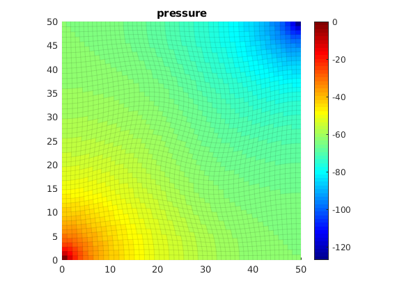
src = addSource([], 1, sum(poreVolume(G,rock)), 'sat', 1);
src = addSource(src, G.cells.num, -sum(poreVolume(G, rock)), 'sat', 1);
Solve pressure equation
Compute transmissibilities and solve pressure equation
trans  = computeTrans(G, rock);
xr = incompTPFA(initResSol(G, 0), G, trans, fluid, 'src', src);
clf,
plotCellData(G,xr.pressure, 'edgecolor','k','edgealpha',.05);
title('pressure')
axis equal tight;colormap jet
colorbar
Compute time-of-flight
Once the fluxes are given, the time-of-flight equation is discretized with a standard upwind finite-volume method
t0 = tic;
T  = computeTimeOfFlight(xr, G, rock, 'src',src);
toc(t0)

clf,
plotCellData(G, T, 'edgecolor','k','edgealpha',0.05);
title('time-of-flight');
caxis([0,0.8]);axis equal tight;colormap jet
colorbar
Elapsed time is 0.006868 seconds.
Copyright notice
<html>
% <p><font size="-1
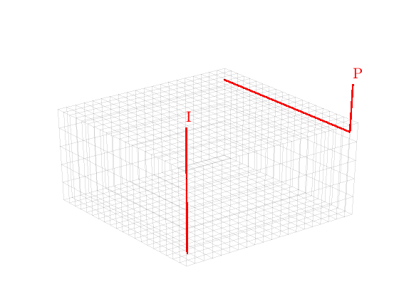
Using Peacemann Well Models
Generated from incompTutorialWells.m
In this example we will demonstrate how our two-point solver can be equipped with a Peacemann type well model. For a vertical well, the model is on the following form

where q is the flow rate p_{bh} is the bottom-hole pressure, r_e is the effective (Peacemann) radius, r_w is the radius of the well, K is the permeability, and h the height of the well. Depending upon what is specified, either the bottom-hole pressure p_bh or the flow rate q end up as extra unknowns per completion in the resulting linear system. To demonstrate the use of well models, we will (as before) solve the single-phase pressure equation
for a Cartesian grid and isotropic, homogeneous permeability. See the basic flow-solver tutorial for more details on the grid structure, the structure used to hold the solutions, etc.
mrstModule add incomp
Define grid, rock and fluid data
Construct a Cartesian grid of size 20-by-20-by-5 cells, where each cell has dimension 1-by-1-by-1. Set permeability equal 100 mD, and use the default single fluid with density 1000 kg/m^3 and viscosity 1 cP.
nx = 20; ny = 20; nz = 5;
G = cartGrid([nx, ny, nz]);
G = computeGeometry(G, 'Verbose', true);
rock = makeRock(G, 100*milli*darcy, 1);
fluid     = initSingleFluid('mu' ,    1*centi*poise     , ...
                            'rho', 1014*kilogram/meter^3);
T = computeTrans(G, rock, 'Verbose', true);
Processing Cells    1 : 2000 of 2000 ... done (0.02 [s], 1.30e+05 cells/second)
Total 3D Geometry Processing Time = 0.017 [s]
Computing one-sided transmissibilities...     Elapsed time is 0.005374 seconds.
Introduce wells
We will include two wells, one rate-controlled vertical well and one horizontal well controlled by bottom-hole pressure. Wells are described using a Peacemann model, giving an extra set of equations that need to be assembled. The first well is vertical well (vertical is default):
cellsWell1 =  1 : nx*ny : nx*ny*nz;
radius     = .1;
W = addWell([], G, rock, cellsWell1, 'Type', 'rate', ...
            'InnerProduct', 'ip_tpf', ...
            'Val', 1.0/day(), 'Radius', radius, 'name', 'I');
disp('Well #1: '); display(W(1));
Well #1:
        cells: [5×1 double]
         type: 'rate'
          val: 1.1574e-05
            r: [5×1 double]
          dir: [5×1 char]
           rR: [5×1 double]
           WI: [5×1 double]
...
The second well is horizontal in the ‘y’ direction:
cellsWell2 = nx : ny : nx*ny;
W = addWell(W, G, rock, cellsWell2, 'Type', 'bhp', ...
            'InnerProduct', 'ip_tpf', ...
            'Val', 1.0e5, 'Radius', radius, 'Dir', 'y', 'name', 'P');
disp('Well #2: '); display(W(2));
Well #2:
        cells: [20×1 double]
         type: 'bhp'
          val: 100000
            r: [20×1 double]
          dir: [20×1 char]
           rR: [20×1 double]
           WI: [20×1 double]
...
We plot the wells to check if the wells are placed as we wanted them. (The plot will later be moved to subplot(2,2,1), hence we first find the corresponding axes position before generating the handle graphics).
subplot(2,2,1), pos = get(gca,'Position'); clf
   plotGrid(G, 'FaceColor', 'none', 'EdgeAlpha',.1);
   view(3), camproj perspective, axis tight off, camlight headlight
   [ht, htxt, hs] = plotWell(G, W, 'radius', radius, 'height', 2);
   set(htxt, 'FontSize', 16);
Once the wells are added, we can generate the components of the linear system corresponding to the two wells and initialize the solution structure (with correct bhp)
resSol = initState(G, W, 0);
display(resSol.wellSol);
1×2 struct array with fields:

    flux
    pressure
Solve linear system
Solve linear system construced from S and W to obtain solution for flow and pressure in the reservoir and the wells.
gravity off
resSol = incompTPFA(resSol, G, T, fluid, 'wells', W);
Warning: Inconsistent Number of Phases. Using 1 Phase (=min([3, 1, 1])).
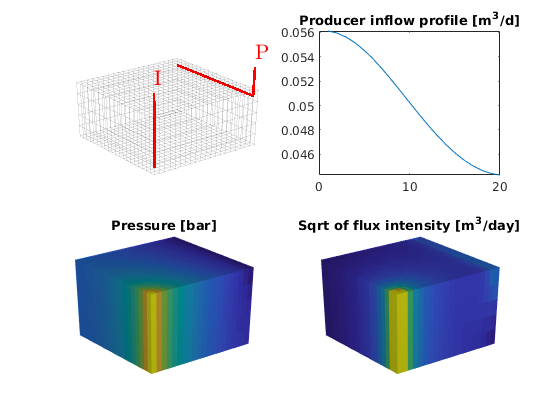
Report results
We move the plot of the grids and wells to the upper-left subplot. The producer inflow profile is shown in the upper-right and the cell pressures in the lower-left subplot. In the lower-right subplot, we show the flux intensity, which must be constructed by averaging over cell faces (this is what is achieved by ‘rldecode’ and ‘accumarray’)
%subplot(2,2,1)
   set(gca, 'Position', pos);  % move the current plot

subplot(2,2,2)
   plot(convertTo(-resSol.wellSol(2).flux, meter^3/day))
   title('Producer inflow profile [m^3/d]');

subplot(2,2,3)
   plotCellData(G, convertTo(resSol.pressure(1:G.cells.num), barsa),'EdgeColor','none');
   title('Pressure [bar]')
   view(3), camproj perspective, axis tight off, camlight headlight

subplot(2,2,4)
   cellNo = rldecode(1:G.cells.num, diff(G.cells.facePos), 2) .';
   cf     = accumarray(cellNo, abs(resSol.flux(G.cells.faces(:,1))) );
   plotCellData(G, convertTo(cf, meter^3/day),'EdgeColor','none' );
   title('Sqrt of flux intensity [m^3/day]')
   view(3), camproj perspective, axis tight off, camlight headlight
Copyright notice
<html>
% <p><font size="-1
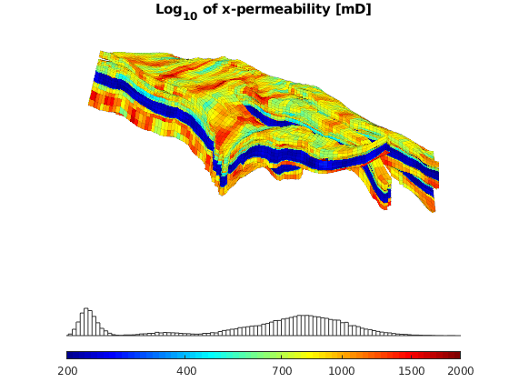
Norne: Two-Phase Incompressible Simulator
Generated from incompExampleNorne2ph.m
In this example we will solve an incompressible two-phase oil-water problem, which consists of an elliptic pressure equation

where v is the Darcy velocity (total velocity) and lambda is the mobility, which depends on the water saturation S. The saturation equation (conservation of the water phase) is given as:
where phi is the rock porosity, f is the Buckley-Leverett fractional flow function, and q_w is the water source term. This is an independent continuation of incompExampleNorne1ph, in which we solved the corresponding single-phase problem for the Norne model, which is a real field from the Norwegian Sea.
mrstModule add incomp
linsolve = @mldivide;
Setup the model
How to read and setup the geological model was discussed in detail in the showNorne and incompExampleNorne1ph tutorials. Here, we therefore just exectute the necessarry commands without further comments,
grdecl = fullfile(getDatasetPath('norne'), 'NORNE.GRDECL');
grdecl = readGRDECL(grdecl);
grdecl = convertInputUnits(grdecl, getUnitSystem('METRIC'));

G = processGRDECL(grdecl); clear grdecl;
G = computeGeometry(G(1));
Set rock and fluid data
The permeability is lognormal and isotropic within nine distinct layers and is generated using our simplified ‘geostatistics’ function and then transformed to lay in the interval 200-2000 mD. For the permeability-porosity relationship we use the simple relationship that phi~0.25*K^0.11, porosities in the interval 0.25-0.32. For the two-phase fluid model, we use values:
gravity off
K          = logNormLayers(G.cartDims, rand([9, 1]), 'sigma', 2);
K          = K(G.cells.indexMap);
K          = 200 + (K-min(K))/(max(K)-min(K))*1800;
rock.perm  = convertFrom(K, milli*darcy);
rock.poro  = 0.25 * (K ./ 200).^0.1;
rock.ntg   = ones(size(K));
fluid      = initSimpleFluid('mu' , [   1,   5]*centi*poise     , ...
                             'rho', [1014, 859]*kilogram/meter^3, ...
                             'n'  , [   2,   2]);
Visualize the model
Set various visualization parameters
myview = struct('vw',   [90, 20],    ...
 % view angle
                'zoom', 1,        ...
 % zoom
                'asp',  [1 1 0.2],  ...
 % data aspect ratio
                'wh',   30,         ...
 % well height above reservoir
                'cb',   'horiz'     ...
 % colorbar location
                );

% Plot the data
clf, title('Log_{10} of x-permeability [mD]');
plotCellData(G,log10(rock.perm),'EdgeColor','k','EdgeAlpha',0.1);
set(gca,'dataasp',myview.asp);
axis off, view(myview.vw); zoom(myview.zoom), colormap(jet), axis tight

cs = [200 400 700 1000 1500 2000];
caxis(log10([min(cs) max(cs)]*milli*darcy));
h = colorbarHist(log10(rock.perm),caxis,'South',100);
set(h, 'XTick', log10(cs*milli*darcy), 'XTickLabel', num2str(cs'));
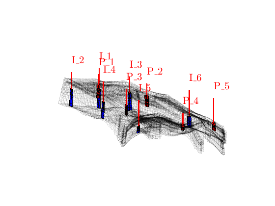
Introduce wells
The reservoir is produced using a set production wells controlled by bottom-hole pressure and rate-controlled injectors. Wells are described using a Peacemann model, giving an extra set of equations that need to be assembled. For simplicity, all wells are assumed to be vertical and are assigned using the logical (i,j) subindex.
% Set vertical injectors, completed in the lowest 12 layers.
nz = G.cartDims(3);
I = [ 9, 26,  8, 25, 35, 10];
J = [14, 14, 35, 35, 68, 75];
R = [ 4,  4,  4,  4,  4,  4]*1000*meter^3/day;
nIW = 1:numel(I); W = [];
for i = 1 : numel(I)
   W = verticalWell(W, G, rock, I(i), J(i), nz-11:nz, 'Type', 'rate', ...
                    'InnerProduct', 'ip_tpf', ...
                    'Val', R(i), 'Radius', 0.1, 'Comp_i', [1, 0], ...
                    'name', ['I$_{', int2str(i), '}$'], ...
                    'RefDepth', 2400*meter);  % Above formation
end

% Set vertical producers, completed in the upper 14 layers
I = [17, 12, 25, 35, 15];
J = [23, 51, 51, 95, 94];
P = [300, 300, 300, 200, 200];
nPW = (1:numel(I))+max(nIW);
for i = 1 : numel(I)
   W = verticalWell(W, G, rock, I(i), J(i), 1:14, 'Type', 'bhp', ...
                    'InnerProduct', 'ip_tpf', ...
                    'Val', 300*barsa(), 'Radius', 0.1, ...
                    'name', ['P$_{', int2str(i), '}$'], ...
                    'Comp_i', [0, 1], 'RefDepth', 2400*meter);
end

% Plot grid outline and the wells
clf
plotGrid(G,'FaceColor','none','EdgeAlpha',0.1);
axis tight off,
view(myview.vw), set(gca,'dataasp',myview.asp), zoom(myview.zoom*.75);
plotWell(G,W,'height',50);
plotGrid(G, vertcat(W(nIW).cells), 'FaceColor', 'b');
plotGrid(G, vertcat(W(nPW).cells), 'FaceColor', 'r');
camdolly(0, .3, 0);
Transmissibilities and initial state
Initialize solution structures and compute transmissibilities from input grid, rock properties, and well structure.
trans = computeTrans(G, rock, 'Verbose', true);
rSol  = initState(G, W, 0, [0, 1]);
Computing one-sided transmissibilities...
Warning:
      137 negative transmissibilities.
      Replaced by absolute values...
Elapsed time is 0.051315 seconds.
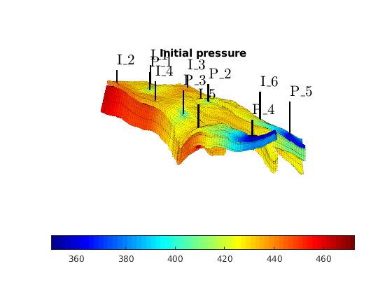
Solve initial pressure
Solve linear system construced from S and W to obtain solution for flow and pressure in the reservoir and the wells.
rSol = incompTPFA(rSol, G, trans, fluid, 'wells', W, ...
                       'LinSolve', linsolve);

clf, title('Initial pressure')
plotCellData(G, convertTo(rSol.pressure(1:G.cells.num), barsa), ...
    'EdgeColor', 'k', 'EdgeAlpha', 0.1);
plotWell(G, W, 'height', myview.wh, 'color', 'k');
axis tight off, view(myview.vw)
set(gca,'dataasp',myview.asp), zoom(myview.zoom*.9)
colorbar(myview.cb), colormap(jet)
camdolly(0,.3,0)
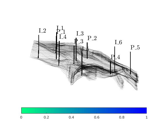
Main loop
In the main loop, we alternate between solving the transport and the flow equations. The transport equation is solved using the standard implicit single-point upwind scheme with a simple Newton-Raphson nonlinear solver.
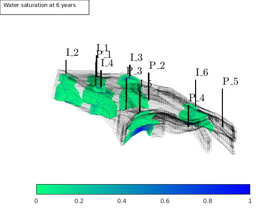
T      = 6*year();
dT     = .5*year;
dTplot = dT;
pv     = poreVolume(G,rock);

% Prepare plotting of saturations
clf
plotGrid(G, 'FaceColor', 'none', 'EdgeAlpha', .1);
plotWell(G, W, 'height', myview.wh, 'color', 'k');
view(myview.vw), set(gca,'dataasp',myview.asp), zoom(myview.zoom/1.2);
axis tight off
h=colorbar(myview.cb); colormap(flipud(winter)),
set(h,'Position',[.13 .07 .77 .05]);
camdolly(0,0.2,0)
[hs,ha] = deal([]); caxis([0 1]);
Start the main loop
t  = 0;  plotNo = 1;
while t < T,
   rSol = implicitTransport(rSol, G, dT, rock, fluid, 'wells', W);

   % Check for inconsistent saturations
   assert(max(rSol.s(:,1)) < 1+eps && min(rSol.s(:,1)) > -eps);

   % Update solution of pressure equation.
   rSol = incompTPFA(rSol, G, trans, fluid, 'wells', W);

    % Increase time and continue if we do not want to plot saturations
   t = t + dT;
   if ( t < plotNo*dTplot && t <T), continue, end

   % Plot saturation
   delete([hs, ha])
   hs = plotCellData(G, rSol.s(:,1), find(rSol.s(:,1) > 0.01),'EdgeColor','none');
   ha = annotation('textbox', [0 0.93 0.32 0.07], ...
                   'String', ['Water saturation at ', ...
                              num2str(convertTo(t,year)), ' years'],'FontSize',8);
   drawnow
   plotNo = plotNo+1;
end
SAIGUP: Solving Two-Phase Flow on a Realistic Corner-Point Model
Generated from incompExampleSAIGUP2ph.m
In this example we will solve an incompressible two-phase oil-water problem, which consists of an elliptic pressure equation
where v is the Darcy velocity (total velocity) and lambda is the mobility, which depends on the water saturation S. The saturation equation (conservation of the water phase) is given as:
where phi is the rock porosity, f is the Buckley-Leverett fractional flow function, and q_w is the water source term. This is an independent continuation of incompExampleSAIGUP1ph, in which we solved the corresponding single-phase problem for the SAIGUP model, which is a synthetic, but realistic model of a shallow-marine reservoir.
mrstModule add incomp
Decide which linear solver to use
- We use MATLAB®’s built-in
mldivide(“backslash”) linear solver software to resolve all systems of linear equations that arise in the various discretzations. In many cases, a multigrid solver such as Notay’s AGMG package may be prefereble. We refer the reader to Notay’s home page at http://homepages.ulb.ac.be/~ynotay/AGMG/ for additional details on this package.
linsolve_p = @mldivide;  % Pressure
linsolve_t = @mldivide;  % Transport (implicit)

% If you have AGMG available
% mrstModule add agmg
% linsolve_p = @agmg;  % Pressure
% linsolve_t = @agmg;  % Transport (implicit)
Setup the model
How to read and setup the geological model was discussed in detail in the showSAIGUP and incompExampleSAIGUP1ph tutorials. Here, we therefore just exectute the necessarry commands without further comments,
grdecl = fullfile(getDatasetPath('SAIGUP'), 'SAIGUP.GRDECL');
grdecl = readGRDECL(grdecl);
grdecl = convertInputUnits(grdecl, getUnitSystem('METRIC'));

G = processGRDECL  (grdecl);
G = computeGeometry(G);

rock = grdecl2Rock(grdecl, G.cells.indexMap);
is_pos                = rock.perm(:, 3) > 0;
rock.perm(~is_pos, 3) = min(rock.perm(is_pos, 3));
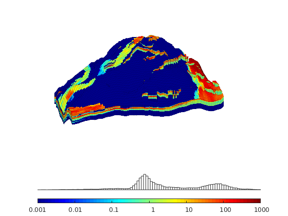
Plot the logarithm of the permeability in the z-direction. The model has a large number of very small permeabilities (shown in dark blue), and in the histogram we have only included permeability values that are larger than 1 micro darcy.
myview = struct('vw',   [-110,18],  ...
 % view angle
                'zoom', 1.0,        ...
 % zoom
                'asp',  [15 15 2],  ...
 % data aspect ratio
                'wh',   50,         ...
 % well height above reservoir
                'cb',   'horiz'     ...
 % colorbar location
                );
K   = rock.perm(:,3);  idx = K>1e-3*milli*darcy;
clf,
plotCellData(G,log10(K),'EdgeColor','k','EdgeAlpha',0.1);
set(gca,'dataasp',myview.asp);
axis off, view(myview.vw); zoom(myview.zoom), colormap(jet)

cs = [0.001 0.01 0.1 1 10 100 1000];
caxis(log10([min(cs) max(cs)]*milli*darcy));
h = colorbarHist(log10(K(idx)),caxis,'South',100);
set(h, 'XTick', log10(cs*milli*darcy), 'XTickLabel', num2str(cs'));
camdolly(.2, 0, 0);
Set fluid data
For the two-phase fluid model, we use values:
gravity off
fluid      = initSimpleFluid('mu' , [   1,   5]*centi*poise     , ...
                             'rho', [1000, 700]*kilogram/meter^3, ...
                             'n'  , [   2,   2]);
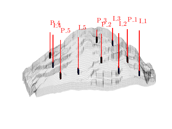
Introduce wells
The reservoir is produced using a set of production wells controlled by bottom-hole pressure and rate-controlled injectors. Wells are described using a Peacemann model, giving an extra set of equations that need to be assembled. For simplicity, all wells are assumed to be vertical and are assigned using the logical (i,j) subindex.
% Set vertical injectors, completed in the lowest 12 layers.
nz = G.cartDims(3);
I = [ 9,  8, 25, 25, 10];
J = [14, 35, 35, 95, 75];
R = [ 4,  4,  4,  4,  4,  4]*125*meter^3/day;
nIW = 1:numel(I); W = [];
for i = 1 : numel(I),
   W = verticalWell(W, G, rock, I(i), J(i), nz-11:nz, 'Type', 'rate', ...
                    'InnerProduct', 'ip_tpf', ...
                    'Val', R(i), 'Radius', 0.1, 'Comp_i', [1, 0], ...
                    'name', ['I$_{', int2str(i), '}$']);
end

% Set vertical producers, completed in the upper 14 layers
I = [17, 12, 25, 33, 7];
J = [23, 51, 51, 95, 94];
nPW = (1:numel(I))+max(nIW);
for i = 1 : numel(I),
   W = verticalWell(W, G, rock, I(i), J(i), 1:14, 'Type', 'bhp', ...
                    'InnerProduct', 'ip_tpf', ...
                    'Val', 300*barsa(), 'Radius', 0.1, ...
                    'name', ['P$_{', int2str(i), '}$'], 'Comp_i', [0, 1]);
end

% Plot grid outline and the wells
clf
plotGrid(G,'FaceColor','none','EdgeAlpha',0.1);
axis tight off,
view(myview.vw), set(gca,'dataasp',myview.asp), zoom(myview.zoom);
plotWell(G,W,'height',50);
plotGrid(G, vertcat(W(nIW).cells), 'FaceColor', 'b');
plotGrid(G, vertcat(W(nPW).cells), 'FaceColor', 'r');
Compute transmissibilities and init reservoir
trans = computeTrans(G, rock, 'Verbose', true);
rSol  = initState(G, W, 0, [0, 1]);
Computing one-sided transmissibilities...
Warning:
      21703 negative transmissibilities.
      Replaced by absolute values...
Elapsed time is 0.092053 seconds.
Construct pressure and transport solvers
solve_press  = @(x) incompTPFA(x, G, trans, fluid, 'wells', W, ...
                                    'LinSolve', linsolve_p);
solve_transp = @(x, dt) ...
   implicitTransport(x, G, dt, rock, fluid, ...
                     'wells', W, 'LinSolve', linsolve_t);
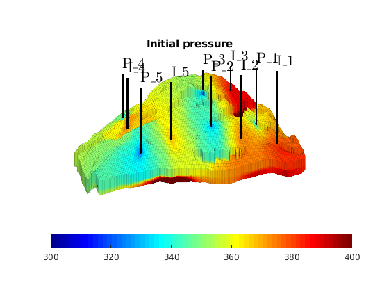
Solve initial pressure
Solve linear system construced from S and W to obtain solution for flow and pressure in the reservoir and the wells.
rSol = solve_press(rSol);

clf, title('Initial pressure')
plotCellData(G, convertTo(rSol.pressure(1:G.cells.num), barsa), ...
    'EdgeColor', 'k', 'EdgeAlpha', 0.1);
plotWell(G, W, 'height', myview.wh, 'color', 'k');
axis tight off, view(myview.vw)
set(gca,'dataasp',myview.asp), zoom(myview.zoom), camdolly(.1,.15,0)
caxis([300 400]), colorbar(myview.cb), colormap(jet)
Main loop
In the main loop, we alternate between solving the transport and the flow equations. The transport equation is solved using the standard implicit single-point upwind scheme with a simple Newton-Raphson nonlinear solver.
T      = 12*year();
dT     = year();
dTplot = year();
pv     = poreVolume(G,rock);

% Prepare plotting of saturations
clf
plotGrid(G, 'FaceColor', 'none', 'EdgeAlpha', .1);
plotWell(G, W, 'height', myview.wh, 'color', 'k');
view(myview.vw), set(gca,'dataasp',myview.asp), zoom(myview.zoom);
axis tight off
h=colorbar(myview.cb); colormap(flipud(winter)),
set(h,'Position',[.13 .07 .77 .05]);
camdolly(.05,0,0)
[hs,ha] = deal([]); caxis([0 1]);

% Start the main loop
t  = 0;  plotNo = 1;
while t < T,
   rSol = solve_transp(rSol, dT);

   % Check for inconsistent saturations
   assert(max(rSol.s(:,1)) < 1+eps && min(rSol.s(:,1)) > -eps);

   % Update solution of pressure equation.
   rSol = solve_press(rSol);

    % Increase time and continue if we do not want to plot saturations
   t = t + dT;
   if ( t < plotNo*dTplot && t <T), continue, end

   % Plot saturation
   delete([hs, ha])
   hs = plotCellData(G, rSol.s(:,1), find(rSol.s(:,1) > 0.01),'EdgeColor','none');
   ha = annotation('textbox', [0 0.93 0.32 0.07], ...
                   'String', ['Water saturation at ', ...
                              num2str(convertTo(t,year)), ' years'],'FontSize',8);
   drawnow
   plotNo = plotNo+1;

end
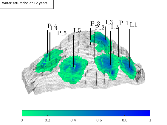
<html>
% <p><font size="-1
Interopability between incomp solvers and ad-props fluids
Generated from incompExampleWithADFluids.m
We can use the fluid models that are used in the ad-blackoil and ad-core modules with the various incompressible solvers. This example demonstrates this on a simple synthetic test problem.
mrstModule add ad-blackoil ad-core ad-props mrst-gui
Set up model
We set up a 1D Buckley-Leverett problem to have something to test.
% Build grid
G = cartGrid([50, 1, 1], [100, 10, 10]*meter);
G = computeGeometry(G);

% Homogenous rock properties
rock = makeRock(G, 5*darcy, .3);

% Default oil-water fluid with unit values
fluid = initSimpleADIFluid('phases', 'WO', 'n', [2 2]);
% Comment out the next line to get a very strong capillary pressure term
% (not suitable for explicitTransport).
% fluid.pcOW = @(s, varargin) -50*s*barsa;

% Set up model and initial state.
model = TwoPhaseOilWaterModel(G, rock, fluid);
state0 = initResSol(G, 50*barsa, [0, 1]);

% Set up drive mechanism: constant rate at x=0, constant pressure at x=L
pv = poreVolume(G, rock);
time = 10000*day;
injRate = sum(pv)/time;
W = [];
W = addWell(W, G, rock, 1, 'type', 'rate', 'val', injRate, 'comp_i', [1, 0]);
W = addWell(W, G, rock, G.cells.num, 'type', 'bhp', 'val', 0, 'comp_i', [1, 0]);
Solve with ad-blackoil fully-implicit solver
We first solve the problem with the fully-implicit solvers.
n  = 100;
dT = time/n;
schedule = simpleSchedule(repmat(dT,1,n), 'W', W);
[~, states, report] = simulateScheduleAD(state0, model, schedule);
Solving timestep 001/100:                    -> 100 Days
Solving timestep 002/100: 100 Days           -> 200 Days
Solving timestep 003/100: 200 Days           -> 300 Days
Solving timestep 004/100: 300 Days           -> 1 Year, 35 Days
Solving timestep 005/100: 1 Year, 35 Days    -> 1 Year, 135 Days
Solving timestep 006/100: 1 Year, 135 Days   -> 1 Year, 235 Days
Solving timestep 007/100: 1 Year, 235 Days   -> 1 Year, 335 Days
Solving timestep 008/100: 1 Year, 335 Days   -> 2 Years, 70 Days
...
Solve using incomp module
We can now solve the same problem with the incomp module. The different incompressible solvers will work directly with fluids from ad-props, under a few limiting assumptions: - The two-phase system is assumed to be a water-oil system where the gas phase will be ignored if present in fluid. Consequently, only pcOW, krO, krOW and krW will be used and pcOG and krG is ignored. - It is not recommended that the fluid model is compressible as the incomp solvers do not account for these nonlinear effects. We still evaluate the b-factors at the given pressure in state (or 1 atmosphere if no pressure is present in state) to obtain the densities. - The explicit transport solver does not handle spatial changes in phase viscosity when estimating CFL. - Fluid regions are not supported by the incomp solvers.
mrstModule add incomp
% Choices for pressure
pressure_discretization = 'tpfa';
% pressure_discretization = 'mpfa';
% pressure_discretization = 'mimetic';

% Choices for transport
transport_discretization = 'implicit';
% transport_discretization = 'explicit';
state = state0;
states_incomp = cell(n, 1);

switch pressure_discretization
    case 'tpfa'
        T = computeTrans(G, rock);
        psolve = @(state) incompTPFA(state, G, T, fluid, 'W', W);
    case 'mpfa'
        mrstModule add mpfa
        T = computeMultiPointTrans(G, rock);
        psolve = @(state) incompMPFA(state, G, T, fluid, 'W', W);
    case 'mimetic'
        IP = computeMimeticIP(G, rock);
        psolve = @(state) incompMimetic(state, G, IP, fluid, 'W', W);
    otherwise
        error('Unknown pressure solver %s', p_solve);
end

switch transport_discretization
    case 'explicit'
        tsolve = @(state, dT) explicitTransport(state, G, dT, rock, fluid, 'W', W);
        substeps = 10;
    case 'implicit'
        tsolve = @(state, dT) implicitTransport(state, G, dT, rock, fluid, 'W', W);
        substeps = 1;
    otherwise
        error('Unknown transport solver %s', transport_discretization);
end
% Solve with a loop
for i = 1:n
    state = psolve(state);
    for j = 1:substeps
        state = tsolve(state, dT/substeps);
    end
    states_incomp{i} = state;
end
Compare the results
We compare the results of the two solvers. The results will agree up to the choice of time integration (our AD solver is fully-implicit, while the incomp module uses either IMPES (implicit pressure, explicit transport) or IMPSAT (implicit pressure, implicit saturation sequentially).
solvename = ['Incomp (', pressure_discretization, '-', transport_discretization, ')'];
x = G.cells.centroids(:, 1);
for i = 1:n
    figure(1); clf; hold on
    plot(x, states{i}.s(:, 1));
    plot(x, states_incomp{i}.s(:, 1), 'o');
    ylim([0, 1]);
    legend('Fully-implicit AD', solvename)
end
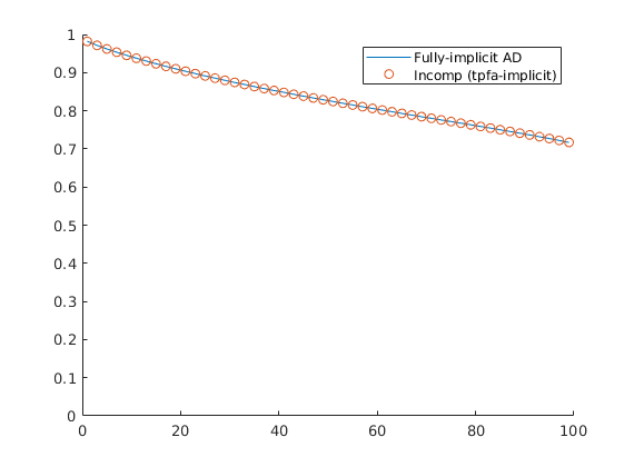
Pressure Solver with capillary pressure:
Generated from incompTutorialCapPres.m
Here, we demonstrate the effect of capillary pressure on the solution of a two-phase oil-water problem. We solve the two-phase pressure equation

where v is the Darcy velocity (total velocity) and lambda_t is the total mobility, which depends on the water saturation S. The saturation equation (conservation of the water phase) is given as:
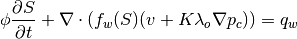
This tutorial shows a 2D case with homogeneous permeability and porosity and linear capillary pressure curve and is based on the incompTutorialWells2ph example.
mrstModule add incomp
verbose = true;
Construct simple Cartesian test case
nx = 40; ny = 40; nz = 1;
G         = cartGrid([nx ny nz]);
G         = computeGeometry(G);
rock      = makeRock(G, 100*milli*darcy, 0.3);
hT  = computeTrans(G, rock, 'Verbose', verbose);
Computing one-sided transmissibilities... Elapsed time is 0.003070 seconds.
Define fluid and capillary pressure curve
We define the relative permeability and the capillary pressure in form of tables, and let the relative permeability curves be quadratic and the capillary function linear. The strength of the capillary pressure is decided by cap_scale. The capillary pressure is defined in the non-wetting phase, i.e.
.
pc_form = 'nonwetting';
cap_scale = 10;
x = linspace(0, 1, 11) .';
y = linspace(1, 0, 11) .';
[kr, pc]  = tabulatedSatFunc([x, x.^2, y.^2, y.*cap_scale*barsa]);

clf,
subplot(1,2,1), plot(x,kr(x),'LineWidth',2); title('Relative permeability');
subplot(1,2,2), plot(x,pc(x),'LineWidth',2); title('Capillary function');

% Define constant properties for viscosity and density
props = constantProperties([   1,  10] .* centi*poise, ...
                           [1000, 700] .* kilogram/meter^3);
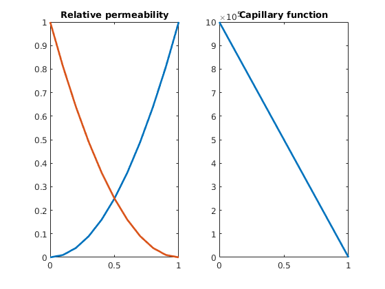
Here we put together a valid fluid object from the above defined functions. To read more about the fluid structure write help fluid_structure in MRST. First make a fluid without capillary pressure
fluid = struct('properties', props                  , ...
               'saturation', @(x, varargin)    x.s  , ...
               'relperm'   , kr);
Then make another fluid object identical to the one above except for the capillary pressure term ‘pc’.
fluid_pc = struct('properties', props                  , ...
                  'saturation', @(x, varargin)    x.s  , ...
                  'relperm'   , kr                     , ...
                  'pc'        , @(x, varargin) pc(x.s));
Plot the pc-curve
Make a dummy state/solution structure to plot the pc curve since ‘fluid.pc’ demands state as an input
xDummy   = initState(G, [], [0, 1]);
xDummy.s = linspace(0, 1, numel(xDummy.s))'; ...
pc = convertTo(fluid_pc.pc(xDummy), barsa);

clf
plot(xDummy.s, pc, 'LineWidth',2);
xlabel('s_w'); ylabel('pc [bar]');
title('Capillary pressure curve')
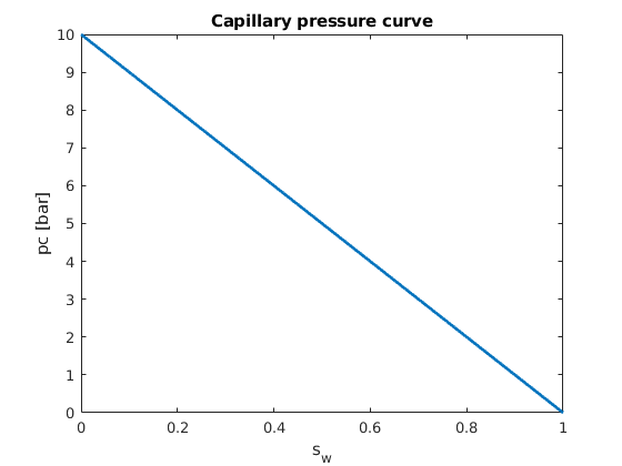
Set wells and ininitialize reservoir state
rate = 0.5*meter^3/day;
bhp  = 1*barsa;
W = verticalWell([], G, rock, 1, 1, 1:nz,          ...
                 'InnerProduct', 'ip_tpf', ...
                 'Type', 'rate', 'Val', rate, ...
                 'Radius', .1, 'Name', 'I', 'Comp_i', [1 0]);
W = verticalWell(W, G, rock, nx, ny, 1:nz,     ...
                 'InnerProduct', 'ip_tpf', ...
                 'Type','bhp', 'Val', bhp, ...
                 'Radius', .1, 'Dir', 'x', 'Name', 'P', 'Comp_i', [0 1]);

rSol    = initState(G, W, 0, [0.2, 0.8]);
rSol_pc = initState(G, W, 0, [0.2, 0.8]);
gravity off
verbose = false;
Set up pressure and transport solvers
This example uses an implicit transport solver, an explicit solver can be used if the time step restriction for the parabolic term is less than for the hyperbolic term. This is the case if ‘cap_scale’ is small. We let ‘fluid’ be a parameter in ‘psolve’ and ‘tsolve’ so that we can use the solvers for simulation both with and without capillary pressure by supplying different fluid objects. For this case we use the verbose = false for the transport solver. If more information about the convergence of the method is required; use verbose = true.
psolve  = @(state, fluid) ...
    incompTPFA(state, G, hT, fluid, 'wells', W);
tsolve  = @(state, dT, fluid) ...
    implicitTransport(state, G, dT, rock, fluid, 'wells', W, 'verbose', verbose);
%
% Alternatively we could have defined an explicit transport solver by
% tsolve = @(state, dT) ...
%     explicitTransport(state, G, dT, rock, fluid, 'wells', W, 'verbose', verbose);
Solve initial pressure in reservoir
Observe that we supply different fluid objects for the two solutions, one with capillary pressure and one without.
rSol    = psolve(rSol, fluid);
rSol_pc = psolve(rSol_pc, fluid_pc);
Transport loop
We solve the two-phase system using a sequential splitting in which the pressure and fluxes are computed by solving the flow equation and then held fixed as the saturation is advanced according to the transport equation.
T      = 300*day();
dT     = T/15;
dTplot = 100*day();  % plot only every 100th day
N      = fix(T/dTplot);
pv     = poreVolume(G,rock);
Start the main loop
t  = 0; plotNo = 1;
h1 = 'No pc - '; h2 = 'Linear pc - ';
e = []; p_org = []; p_pc = [];
clf;

while t < T,
   % TRANSPORT SOLVE
   rSol    = tsolve(rSol, dT, fluid);
   rSol_pc = tsolve(rSol_pc, dT, fluid_pc);

   % Check for inconsistent saturations
   s = [rSol.s(:,1); rSol_pc.s(:,1)];
   assert(max(s) < 1+eps && min(s) > -eps);

   % Update solution of pressure equation.
   rSol    = psolve(rSol,    fluid);
   rSol_pc = psolve(rSol_pc, fluid_pc);

   % Measure water saturation in production cells in saturation
   e = [e; sum(abs(rSol.s(:,1) - rSol_pc.s(:,1)).*pv)/sum(pv)]; %#ok
   p_org = [p_org; rSol.s(W(2).cells,1)' ];                 %#ok
   p_pc  = [p_pc; rSol_pc.s(W(2).cells,1)'];                 %#ok

   % Increase time and continue if we do not want to plot saturations
   t = t + dT;
   if ( t < plotNo*dTplot && t <T), continue, end

   % Plot saturation
   heading = [num2str(convertTo(t,day)),  ' days'];
   r = 0.01;
   subplot('position',[(plotNo-1)/N+r, 0.50, 1/N-2*r, 0.48]), cla
   plotCellData(G, rSol.s(:,1),'EdgeColor','none');
   caxis([0 1]), view(60,50), axis tight off, set(gca,'dataasp',[12 12 1]),
   title([h1 heading])

   subplot('position',[(plotNo-1)/N+r, 0.02, 1/N-2*r, 0.48]), cla
   plotCellData(G, rSol_pc.s(:,1),'EdgeColor','none');
   caxis([0 1]), view(60,50), axis tight off, set(gca,'dataasp',[12 12 1]),
   title([h2 heading])
   drawnow

   plotNo = plotNo+1;

end
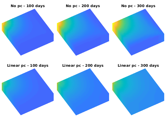
Plot water breakthrough at heel
As we clearly see from the plots in the figure, the simulation with capillary pressure has much more diffusion than the simulation without capillary pressure. This is confirmed by the water breakthrough curve.
clf
n = numel(p_org(:,1));
plot(1:n,p_org(:,1),'-o',1:n,p_pc(:,1),'--s','MarkerSize',8,'MarkerFaceColor',[.7 .7 .7])
legend('No capillary pressure','Linear capillary pressure','Location','Best');
axis tight
title('Water breakthrough at heel');
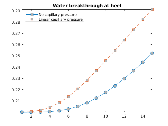
Copyright notice
<html>
% <p><font size="-1
Two-Phase Flow in Inclined Gravity Column
Generated from incompTutorialGravCol2ph.m
In this example, we simulate the injection of a light fluid (CO2) into a heavier fluid (brine) inside an inclined sandbox.
mrstModule add incomp
Set up model
To get an inclined reservoir, we manipulate the gravity direction. Since gravity is a persistent and global variable, it is important that we reset the gravity at the end of the script
rotdeg = 40;
height = 40;
n      = [ 20,  2,  100];
box_sz = [100, 10, 200];
G      = cartGrid(n, box_sz); CG = cartGrid([1 1 1],box_sz);
G      = computeGeometry(G);
rock   = makeRock(G, 0.1*darcy, 0.3);
T      = computeTrans(G, rock, 'verbose', true);

fluid  = initSimpleFluid('mu' , [  0.307,   0.049] .* centi*poise     , ...
                         'rho', [973    , 617    ] .* kilogram/meter^3, ...
                         'n'  , [  2    ,   2    ]);

% Redefine gravity direction
rot   = @(theta) makehgtform('xrotate',  theta(1), ...
                             'yrotate', -theta(2), ...
                             'zrotate', -theta(3));
mul   = @(a,b,n) a(1:n,1:n) * reshape(b(1:n), [], 1);
angle = [0, pi*rotdeg/180, 0];
gravity reset on
gravity(mul(rot(angle), gravity(), 3));
Computing one-sided transmissibilities... Elapsed time is 0.004824 seconds.
Compute initial pressure distribution
Put region of CO2 at bottom of reservoir.
xr = initResSol(G, 1*barsa, 1);
d  = gravity() ./ norm(gravity);
dc = G.cells.centroids * d.';
xr.s(dc>max(dc)-height) = 0;
xr = incompTPFA(xr, G, T, fluid);

cla reset
h = plotCellData(G, convertTo(xr.pressure(1:G.cells.num), barsa), ...
                 'EdgeColor', 'k', 'EdgeAlpha', 0.1, 'FaceAlpha', 0.625);
rotate(h,[0 1 0],rotdeg);
view([0,0]), axis equal tight off
colorbar, colormap(jet(10))
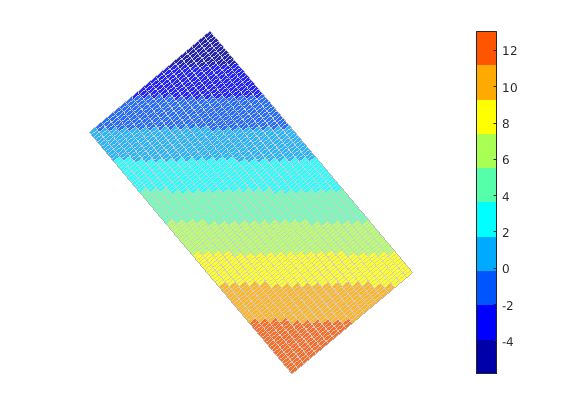
Prepare to plot during simulation
clf
h = plotGrid(CG, 'FaceColor', 'none', 'EdgeColor', 'k','LineWidth',1);
rotate(h,[0 1 0],rotdeg);
view([0,0]), axis tight off
hs = plotCellData(G, xr.s, xr.s < .995, 'EdgeColor', 'none');
rotate(hs,[0 1 0],rotdeg);
s  = linspace(0, 1, 64).';
cm = [1-s.^(13/16), 1-s.^6, s.^6];
caxis([0 1]); colormap(cm), colorbar, axis equal
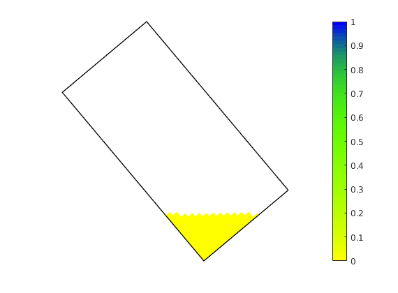
Run simulation
For accuracy, the time step is gradually ramped up
dT = [.5, .5, 1, 1, 1, 2, 2, 2, 5, 5, 10, 10, 15, 20, repmat(25,[1,97])].*day();
t = 0;
for k = 1 : numel(dT),
   xr = implicitTransport(xr, G, dT(k), rock, fluid, 'Verbose', false);

   % Check for inconsistent saturations
   assert (max(xr.s) < 1+eps && min(xr.s) > -eps);

   % Increase time and plot saturation
   t = t + dT(k);
   delete(hs)
   hs = plotCellData(G, xr.s, xr.s <.995, 'EdgeColor', 'none');
   rotate(hs,[0 1 0],rotdeg);
   title(sprintf('%.2f days', t/day));
   drawnow

   % Compute new flow field.
   xr = incompTPFA(xr, G, T, fluid);
end
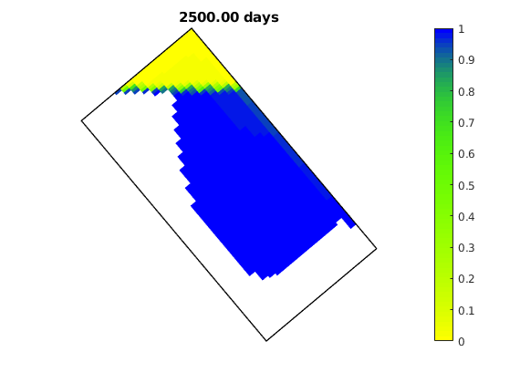
NB: RESET GRAVITY
Gravity is defined as a persistent and global variable and we therefore need to reset it to avoid messing with other examples
gravity reset on
Basic Transport-Solver Tutorial
Generated from incompTutorialWells2ph.m
Consider a two-phase oil-water problem. Solve the two-phase pressure equation
where v is the Darcy velocity (total velocity) and lambda is the mobility, which depends on the water saturation S. The saturation equation (conservation of the water phase) is given as:
where phi is the rock porosity, f is the Buckley-Leverett fractional flow function, and q_w is the water source term. This is a continuation of the incompIntro flow-solver tutorial</a>, in which we solved the corresponding single-phase problem using the two-point pressure solver. Here, we demonstrate how this flow solver can be extended by an explicit or an implicit two-phase transport solver. The grid is Cartesian with isotropic, homogeneous permeability. See the basic flow-solver tutorial</a for more details on the grid structure, the structure used to hold the solutions, etc.
mrstModule add incomp
Define geometry and rock parameters
Construct a Cartesian grid of size 20-by-20-by-5 cells, where each cell has dimension 1-by-1-by-1. Set the permeability K to be homogeneous, isotropic and equal 100 mD and the porosity to be equal to 0.3. Compute one-sided (half) transmissibilities from input grid and rock properties.
nx = 20; ny = 20; nz = 5;
G = cartGrid([nx, ny, nz]);
G = computeGeometry(G);

rock.perm  = 100*milli*darcy*ones(G.cells.num, 1);
rock.poro  = .3*ones(G.cells.num, 1);
rock.ntg   = ones(G.cells.num, 1);

hT  = computeTrans(G, rock, 'Verbose', true);
Computing one-sided transmissibilities... Elapsed time is 0.005086 seconds.
Define the two-phase fluid model
The two-phase fluid model has default values:
fluid = initSimpleFluid('mu' , [   1,  10] .* centi*poise     , ...
                        'rho', [1000, 700] .* kilogram/meter^3, ...
                        'n'  , [   2,   2]);
The fluid model represented by the fluid structure is the two-phase incompressible counterpart to the fluid models used in the black-oil framework
s=linspace(0,1,20)'; kr=fluid.relperm(s);
plot(s, kr(:,1), 'b', s, kr(:,2), 'r', 'LineWidth',2);
title('Relative permeability curves')
legend('Water','Oil','Location','Best')
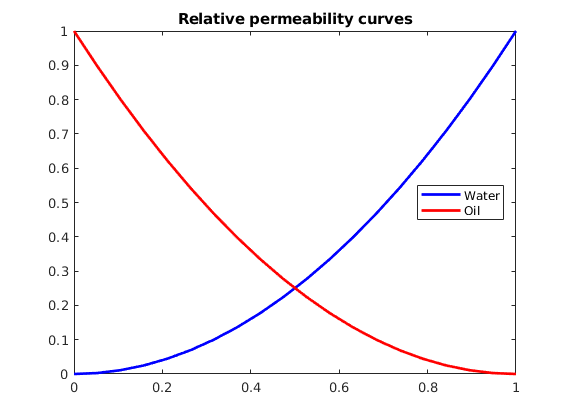
Introduce wells
We will include two wells, one rate-controlled vertical well and one horizontal well controlled by bottom-hole pressure. Wells are described using a Peacemann model, giving an extra set of equations that need to be assembled, see the tutorial on well models for more details.
W = addWell([], G, rock, 1 : nx*ny : nx*ny*nz,          ...
            'InnerProduct', 'ip_tpf', ...
            'Type', 'rate', 'Val', 1.0/day(), ...
            'Radius', 0.1, 'Comp_i', [1, 0]);
W = addWell(W, G, rock, nx : ny : nx*ny, ...
            'InnerProduct', 'ip_tpf', ...
            'Type', 'bhp' , 'Val', 1.0e5, ...
            'Radius', 0.1, 'Dir', 'y', 'Comp_i', [0, 1]);

% To check if the wells are placed as we wanted them, we plot them
clf
plotGrid(G, 'FaceColor', 'none'); view(3);
[ht, htxt, hs] = plotWell(G, W, 'radius', 0.1, 'height', 2);
set(htxt, 'FontSize', 16);
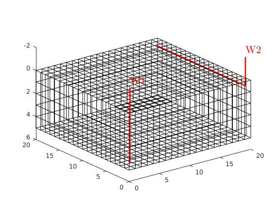
Once the wells are added, we can generate the components of the linear system corresponding to the two wells and initialize the solution structure (with correct bhp)
rSol = initState(G, W, 0, [0, 1]);
Solve initial pressure in reservoir
Solve linear system construced from S and W to obtain solution for flow and pressure in the reservoir and the wells.
gravity off
rSol = incompTPFA(rSol, G, hT, fluid, 'wells', W);

% Report initial state of reservoir
subplot(2,1,1), cla
   plotCellData(G, convertTo(rSol.pressure(1:G.cells.num), barsa));
   title('Initial pressure'), view(3)

subplot(2,1,2), cla
   cellNo = rldecode(1:G.cells.num, diff(G.cells.facePos), 2) .';
   plotCellData(G, accumarray(cellNo, ...
      abs(convertTo(faceFlux2cellFlux(G, rSol.flux), meter^3/day))));
   title('Initial flux intensity'), view(3)
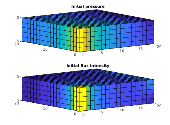
Transport loop
We solve the two-phase system using a sequential splitting in which the pressure and fluxes are computed by solving the flow equation and then held fixed as the saturation is advanced according to the transport equation. This procedure is repeated for a given number of time steps (here we use 15 equally spaced time steps). The error introduced by this splitting of flow and transport can be reduced by iterating each time step until e.g., the residual is below a certain user-prescribed threshold (this is not done herein).
T      = 300*day();
dT     = T/15;
dTplot = 100*day();  % plot only every 100th day
N      = fix(T/dTplot);
pv     = poreVolume(G,rock);
The transport equation will be solved by the single-point upstream method with either explicit or implicit time discretizations. Both schemes may use internal time steps to obtain a stable discretization. To represent the two solutions, we create new solution objects to be used by the solver with implicit transport step.
rISol = rSol;
Start the main loop
t  = 0; plotNo = 1; hi = 'Implicit: '; he = 'Explicit: ';
e = []; pi = []; pe = [];
while t < T,
   rSol  = explicitTransport(rSol , G, dT, rock, fluid, 'wells', W);
   rISol = implicitTransport(rISol, G, dT, rock, fluid, 'wells', W);

   % Check for inconsistent saturations
   s = [rSol.s(:,1); rISol.s(:,1)];
   assert(max(s) < 1+eps && min(s) > -eps);

   % Update solution of pressure equation.
   rSol  = incompTPFA(rSol , G, hT, fluid, 'wells', W);
   rISol = incompTPFA(rISol, G, hT, fluid, 'wells', W);

   % Measure water saturation in production cells in saturation
   e = [e; sum(abs(rSol.s(:,1) - rISol.s(:,1)).*pv)/sum(pv)]; %#ok
   pe = [pe; rSol.s(W(2).cells,1)' ];                 %#ok
   pi = [pi; rISol.s(W(2).cells,1)'];                 %#ok

   % Increase time and continue if we do not want to plot saturations
   t = t + dT;
   if ( t < plotNo*dTplot && t <T), continue, end

   % Plot saturation
   heading = [num2str(convertTo(t,day)),  ' days'];
   r = 0.01;
   subplot('position',[(plotNo-1)/N+r, 0.50, 1/N-2*r, 0.48]), cla
   plotCellData(G, rSol.s(:,1));
   view(60,50), axis equal off, title([he heading])

   subplot('position',[(plotNo-1)/N+r, 0.02, 1/N-2*r, 0.48]), cla
   plotCellData(G, rISol.s(:,1));
   view(60,50), axis equal off, title([hi heading])
   drawnow

   plotNo = plotNo+1;
end
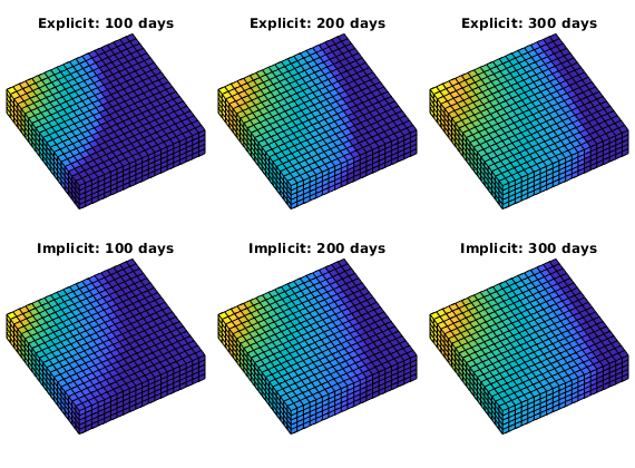
As we clearly can see from the plots in the figure, the implicit scheme has much more numerical diffusion than the explicit scheme early in the simulation, but as the time increase, the difference is smaller. To verify this, we can plot the error or the breakthrough curves
n = size(pe,1);
pargs = {'MarkerSize',6,'MarkerFaceColor',[.5 .5 .5]};
subplot(2,1,1),
   plot(1:n,e*100,'-o', pargs{:}),
   title('Percentage saturation discrepancy')
subplot(2,1,2),
   plot(1:n,pe(:,1),'-o',1:n,pi(:,1),'-s',pargs{:})
   legend('Explicit','Implicit','Location','NorthWest');
   title('Water breakthrough at heel'); axis tight
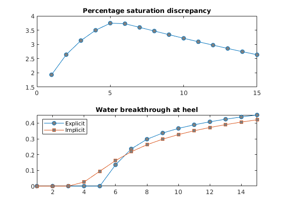
<html>
% <p><font size="-1