`ad-eor`: Enhanced oil recovery solvers¶

The ad-eor module extends the solvers found in ad-core and ad-blackoil with capability for simulating enhanced oil recovery (EOR). EOR is a category of recovery techniques that are characterized by the addition of different chemicals to improve the final recovery. Specifically, the module includes simulation of polymer with mixing rules, dead pore space, adsorption and velocity dependent viscosity, as well as surfactant. ad

Models¶

Base classes¶

Contents¶

MODELS

Files: OilWaterPolymerModel - Oil/water/polymer system OilWaterSurfactantModel - SYNOPSIS: ThreePhaseBlackOilPolymerModel - Three-phase black-oil model with support for polymer injection ThreePhaseBlackOilSurfactantModel - SYNOPSIS: ThreePhaseSurfactantPolymerModel - Three-phase black-oil model with support for surfactant and polymer injection

class OilWaterPolymerModel(G, rock, fluid, varargin)¶

Bases: TwoPhaseOilWaterModel

Oil/water/polymer system

Synopsis:

model = OilWaterPolymerModel(G, rock, fluid, varargin)

Description:

Two phase model with polymer. A description of the polymer model that is implemented here can be found in the directory ad-eor/docs .

Parameters:	G – Grid rock – Rock structure fluid – Fluid structure varargin – optional parameter
Returns:	class instance

EXAMPLE:

SEE ALSO: ThreePhaseBlackOilPolymerModel

addComponentContributions(model, cname, eq, component, src, force)¶

For a given component conservation equation, compute and add in source terms for a specific source/bc where the fluxes have already been computed.

Parameters:

model – (Base class, automatic)
cname – Name of the component. Must be a property known to the model itself through getProp and getVariableField.
eq – Equation where the source terms are to be added. Should be one value per cell in the simulation grid (model.G) so that the src.sourceCells is meaningful.
component – Cell-wise values of the component in question. Used for outflow source terms only.
src – Source struct containing fields for fluxes etc. Should be constructed from force and the current reservoir state by computeSourcesAndBoundaryConditionsAD.
force – Force struct used to produce src. Should contain the field defining the component in question, so that the inflow of the component through the boundary condition or source terms can accurately by estimated.

getVariableField(model, name, varargin)¶: Get the index/name mapping for the model (such as where pressure or water saturation is located in state)

class OilWaterSurfactantModel(G, rock, fluid, varargin)¶

Bases: TwoPhaseOilWaterModel

Synopsis:

model = FullyImplicitOilWaterSurfactantModel(G, rock, fluid, varargin)

Description:

Fully implicit model for an oil water system with surfactant. All the equations are solved implicitly. A description of the surfactant model that is implemented can be found in the directory ad-eor/docs .

Parameters:	G – Grid rock – Rock structure fluid – Fluid structure varargin – optional parameter
Returns:	class instance

EXAMPLE:

Utilities¶

Contents¶

UTILS

Files: addPolymerProperties - Undocumented Utility Function computeCapillaryNumber - SYNOPSIS: computeFluxAndPropsOilWaterSurfactant - SYNOPSIS: computeFluxAndPropsThreePhaseBlackOilSurfactant - SYNOPSIS: computeRelPermSft - SYNOPSIS: computeSqVelocTPFA - SYNOPSIS: computeVelocTPFA - SYNOPSIS: equationsOilWaterPolymer - SYNOPSIS: equationsOilWaterSurfactant - SYNOPSIS: equationsThreePhaseBlackOilPolymer - SYNOPSIS: equationsThreePhaseBlackOilSurfactant - SYNOPSIS: equationsThreePhaseSurfactantPolymer - SYNOPSIS: getFluxAndPropsWaterPolymer_BO - dpW, extraOutput updateAdsorption - SYNOPSIS:

equationsThreePhaseBlackOilSurfactant¶: …

addPolymerProperties(fluid, varargin)¶: Undocumented Utility Function

computeCapillaryNumber(p, c, pBH, W, fluid, G, operators, varargin)¶

Synopsis:

function Nc = computeCapillaryNumber(p, c, pBH, W, fluid, G, operators, varargin)

DESCRIPTION: Computes the capillary number which is equal to the ratio between absolute total velocity and the surface tension. See documentation in the directory ad-eor/docs .

Keyword Arguments:
Parameters:	p – pressure c – concentration pBH – bottom hole pressure W – Well structure fluid – Fluid structure G – Grid operators – discrete differential operator (Grad, T (transmissibilies), …) varargin – optional arguments
	velocCompMethod – if ‘linear’ (default), uses computeVelocTPFA if ‘square’, uses computeSqVelocTPFA
Returns:	Nc – Capillary number

EXAMPLE:

SEE ALSO:

computeFluxAndPropsOilWaterSurfactant(model, p0, p, sW, c, pBH, W, varargin)¶

Synopsis:

function [dpO, dpW, mobO, mobW, upco, upcw, bO, bW, pvMult, bO0, bW0, pvMult0, T] =  computeFluxAndPropsOilWaterSurfactant(model, p0, p, sW, c, pBH, W, varargin)

DESCRIPTION: Given the state variable (pressure, saturation and concentration), compute fluxes and other properties, as listed below.

Parameters:

model – Model instance
p0 – Pressure at previous time step
p – Pressure at current time step
sW – Saturation
c – Surfactant concentration
pBH – bottom hole pressure
W – Well structure
varargin –

Returns:

dpO – Oil pressure gradient (face-valued)
dpW – Water pressure gradient (face-valued)
mobO – Oil mobility
mobW – Water mobility
upco – Upstream direction for oil (face-values)
upcw – Upstream direction for water (face-values)
bO – Oil formation volume factor
bW – water formation volume factor
pvMult – Pore volume multiplier
bO0 – Oil formation volume factor for previous time step
bW0 – Water formation volume factor for previous time step
pvMult0 – Pore volume multiplier for previous time step
T – Transmissibilities

EXAMPLE:

SEE ALSO:

computeFluxAndPropsThreePhaseBlackOilSurfactant(model, p0, p, sW, sG, c, pBH, W, rs, rs0, rv, rv0, st, st0, varargin)¶

Synopsis:

function [p, dpO, dpW, mobO, mobW, upco, upcw, bO, bW, pvMult, bO0, bW0, pvMult0, T] =
computeFluxAndPropsThreePhaseBlackOilSurfactant(model, p0, p, sW, c, pBH, W, rs, rv, st, st0, varargin)

DESCRIPTION: Given the state variable (pressure, saturation and concentration), compute fluxes and other properties, as listed below.

Parameters:

model – Model instance
p0 – Pressure at previous time step
p – Pressure at current time step
sW – Water Saturation
sG – Gas Saturation
c – Surfactant concentration
pBH – bottom hole pressure
W – Well structure
varargin –

Returns:

dpO – Oil pressure gradient (face-valued)
dpW – Water pressure gradient (face-valued)
mobO – Oil mobility
mobW – Water mobility
upco – Upstream direction for oil (face-values)
upcw – Upstream direction for water (face-values)
bO – Oil formation volume factor
bW – water formation volume factor
pvMult – Pore volume multiplier
bO0 – Oil formation volume factor for previous time step
bW0 – Water formation volume factor for previous time step
pvMult0 – Pore volume multiplier for previous time step
T – Transmissibilities

EXAMPLE:

SEE ALSO:

computeRelPermSft(sW, c, Nc, fluid)¶

Synopsis:

function [krW, krO] = computeRelPermSft(sW, c, Nc, fluid)

DESCRIPTION: Computes the water and oil relative permeabilities, using the surfactant model as described in ad-eor/docs/surtactant_model.pdf

Parameters:	sW – Saturation c – Concentration Nc – Capillary number fluid – Fluid structure
Returns:	krW – Water relative permeability krO – Oil relative permeability

EXAMPLE:

SEE ALSO:

computeSqVelocTPFA(G, intInx)¶

Synopsis:

function sqVeloc = computeSqVelocTPFA(G, intInx)

DESCRIPTION: Setup the operator which computes an approximation of the square of the velocity for each cell given fluxes on the faces. The following method is used

1) For each face, we compute a square velocity by taking the square of the flux after having divided it by the area. We obtain a scalar-valued variable per face

2) From a scalar variable, a vector can be reconstructed on each face, using the coordinate of the vector joining the cell centroid to the face centroid. Let c denotes this vector, after renormalization, (example: c=[1;0;0]’ for a face of a Cartesian 3D grid) then, from a scalar value f on the face, we construct the vector-valued variable given by f*c.

3) We use the reconstruction defined in 2) to construct vector-valued square velocity from the scalar-valued square velocity defined in 1).

4) We take the average of the vector-valued obtained in 3) . We use a weight in the average so that faces that are far from the cell centroid contribute less than those that are close. See implementation for how this is done.

Parameters:	G – Grid structure intInx – Logical vector giving the internal faces.
Returns:	sqVeloc – Function of the form u=sqVeloc(v), which returns cell-valued square of the velocity for given face – valued fluxes v.

EXAMPLE:

Examples¶

Computation of Adjoints for Polymer and Waterflooding¶

Generated from adjointWithPolymerExample.m

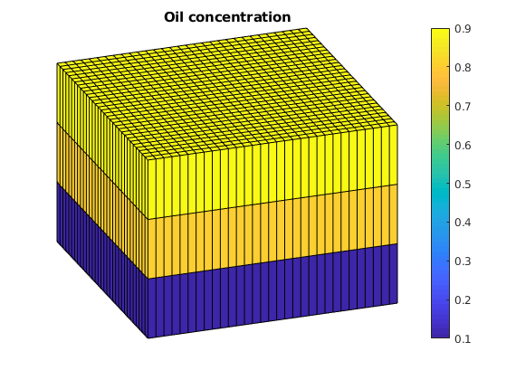
In this example, we demonstrate how one can use an adjoint simulation to compute gradients (sensitivities). To illustrate this, we compare water and polymer flooding in a simple box-shaped reservoir represented on a uniform 31×31×3 Cartesian grid with homogeneous rock properties. The well pattern consists of a producer in the center of the reservoir and two injectors in the northeast and southwest corners; all wells are completed in the top layer. Somewhat unrealistic, the well schedule consists of a period of injection with polymer, followed by a water flooding phase without polymer. Finally, the water rate is reduced for the final time steps. For comparison, we also simulate a case with pure waterflooding. The implementation and computational strategy used to obtain adjoints is independent of the actual system considered and a similar approach can be used for other systems and setups with minor (and obvious) modifications.

mrstModule add ad-core ad-blackoil ad-eor ad-props deckformat optimization

Read input file and setup basic structures¶

The computational setup is described in an input file on the ECLIPSE input format. We start by reading this file and extracting the necessary structures to represent grid, petrophysics, and fluid properties.

current_dir = fileparts(mfilename('fullpath'));
fn  = fullfile(current_dir, 'POLYMER.DATA');

deck = readEclipseDeck(fn);
deck = convertDeckUnits(deck);

G = initEclipseGrid(deck);
G = computeGeometry(G);

rock  = initEclipseRock(deck);
rock  = compressRock(rock, G.cells.indexMap);

fluid = initDeckADIFluid(deck);

% Oil rel-perm from 2p OW system.
% Needed by equation implementation function 'eqsfiOWExplictWells'.
fluid.krO = fluid.krOW;

gravity on

No converter needed in section 'REGIONS'.
No converter needed in section 'SUMMARY'.
Processing Cells    1 : 2883 of 2883 ... done (0.03 [s], 8.92e+04 cells/second)
Total 3D Geometry Processing Time = 0.034 [s]

Set up initial reservoir state¶

Initially, the reservoir is filled by oil on top and water at the bottom. The horizontal oil-water contact passes through the second grid layer and hence we get different saturations in each of the three grid layers.

ijk = gridLogicalIndices(G);
state0 = initResSol(G, 300*barsa, [ .9, .1]);
state0.s(ijk{3} == 1, 2) = .9;
state0.s(ijk{3} == 2, 2) = .8;

% Enforce s_w + s_o = 1;
state0.s(:,1) = 1 - state0.s(:,2);

% Add zero polymer concentration to the state.
state0.cp    = zeros(G.cells.num, 1);
state0.cpmax = zeros(G.cells.num, 1);

clf, title('Oil concentration')
plotCellData(G, state0.s(:,2));
plotGrid(G, 'facec', 'none')
axis tight off, view(70, 30), colorbar;

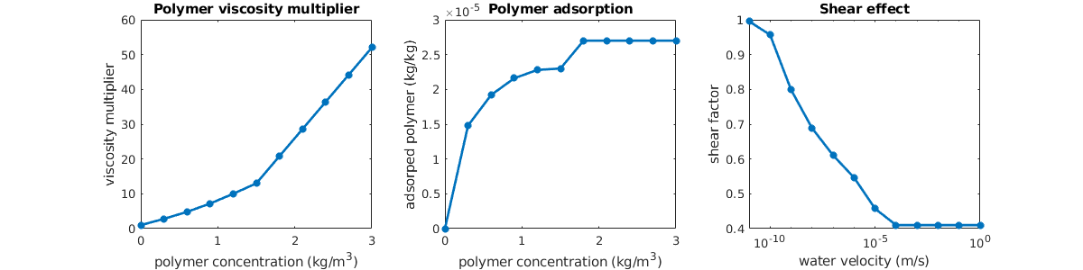
_images/adjointWithPolymerExample_01.png

Plot polymer properties¶

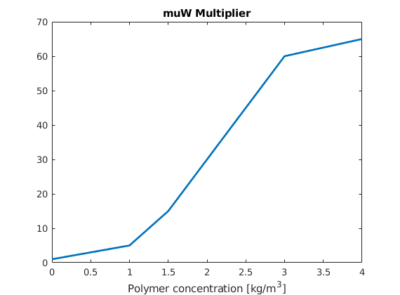
In the basic setup, water is much more mobile than the oil we are trying to displace, and as a result, a pure waterflooding will not be very efficient. To improve the oil recovery, we will add polymer to the injected water phase. This will increase the viscosity of the water phase and hence make the water much less mobile, which in turn will increase the local displacement efficiency and also the volumetric sweep. To see the effect of polymer on the water viscosity, we plot the visocity multiplier, which is based on tabulated data given in the input file

dc = 0 : .1 : fluid.cpmax;
plot(dc, fluid.muWMult(dc),'LineWidth',2)
title('muW Multiplier')
xlabel('Polymer concentration [kg/m^3]')

_images/adjointWithPolymerExample_02.png

Set up systems¶

To quantify the effect of adding the polymer to the injected water, we will solve the same system both with and without polymer. This is done by creating an Oil/Water/Polymer system and an Oil/Water system. Note that since the data file already contains polymer as an active phase, we do not need to pass initADISystem anything other than the deck.

modelPolymer = OilWaterPolymerModel(G, rock, fluid, 'inputdata', deck);
modelOW = TwoPhaseOilWaterModel(G, rock, fluid, 'inputdata', deck);

% Convert the deck schedule into a MRST schedule by parsing the wells
schedule = convertDeckScheduleToMRST(modelPolymer, deck);

Ordering well 1 (INJE1) with strategy "origin".
Ordering well 2 (INJE2) with strategy "origin".
Ordering well 3 (PROD) with strategy "origin".

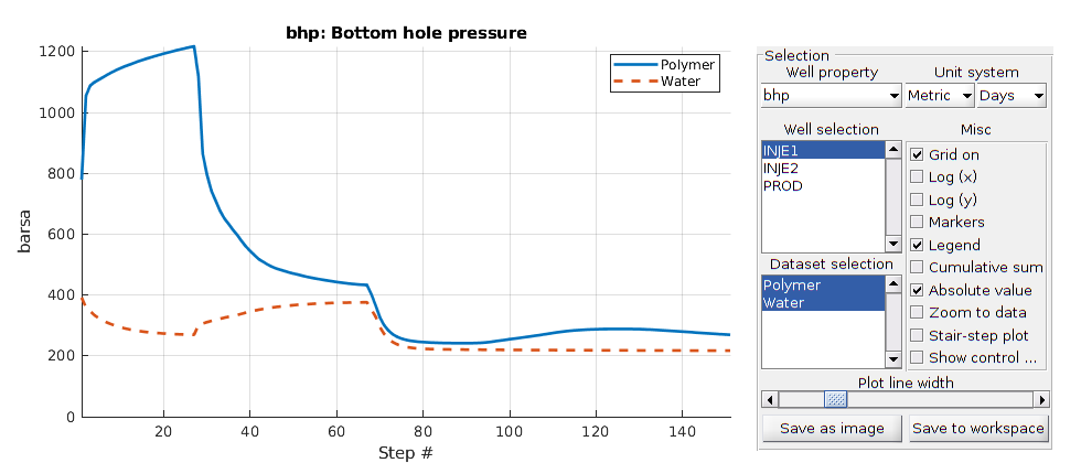
Run the schedule¶

Once a model has been created it is trivial to run the schedule. Any options such as maximum non-linear iterations and tolerance can be set in the model and the NonLinearSolver class (optional argument to simulateScheduleAD).

[wellSolsPolymer, statesPolymer] = simulateScheduleAD(state0, modelPolymer, ...
                                                  schedule);

*****************************************************************
********** Starting simulation:   151 steps,  2494 days *********
*****************************************************************
Preparing model for simulation...
Model ready for simulation...
Preparing schedule for simulation...
Schedule ready for simulation...
Validating initial state...
...

[wellSolsOW, statesOW] = simulateScheduleAD(state0, modelOW, schedule);

plotWellSols({wellSolsPolymer; wellSolsOW},'datasetnames',{'Polymer','Water'});

*****************************************************************
********** Starting simulation:   151 steps,  2494 days *********
*****************************************************************
Preparing model for simulation...
Model ready for simulation...
Preparing schedule for simulation...
Schedule ready for simulation...
Validating initial state...
...

_images/adjointWithPolymerExample_03.png

Objective functions¶

Create objective functions for the different systems. We set up approximate prices in USD for both the oil and the injection cost of the different phases. The polymer injection cost is per kg injected.

prices = {'OilPrice',            100  , ...
          'WaterProductionCost',   1  , ...
          'WaterInjectionCost',    0.1, ...
          'DiscountFactor',        0.1 };

objectivePolymerAdjoint = ...
    @(tstep) NPVOWPolymer(G, wellSolsPolymer, schedule, ...
                          'ComputePartials', true, 'tStep', tstep, ...
                          prices{:});

% We first calculate the NPV of the pure oil/water solution.
objectiveOW = NPVOW(G, wellSolsOW, schedule, prices{:});

% Calculate the objective function for three different polymer prices
objectivePolymer = ...
    @(polyprice) NPVOWPolymer(G, wellSolsPolymer, schedule, prices{:}, ...
                              'PolymerInjectionCost', polyprice);

objectiveInexpensivePolymer = objectivePolymer( 1.0);
objectiveRegularPolymer     = objectivePolymer( 5.0);
objectiveExpensivePolymer   = objectivePolymer(15.0);

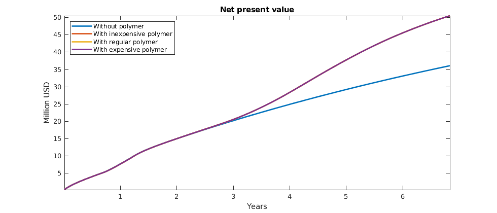
Plot accumulated present value¶

The objective function is now the net present value of the reservoir at each time step, i.e. the cost of doing that timestep. However, the most interesting value is here the accumulated net present value, as it will show us the profit over the lifetime of the reservoir. We plot the three different polymer costs, as well as the total profit without polymer injection. While polymer is injected, the net present value may be lower than without polymer as there is an increased cost. Once the polymer injection phase is over, however, we hope to reap the benefits and get an increased oil output resulting in a bigger total value for the reservoir lifetime.

figure(gcf); clf;
cumt = cumsum(schedule.step.val);
v = @(value) cumsum([value{:}]);

plot(convertTo(cumt, year), ...
     convertTo([v(objectiveOW)            ; ...
                v(objectiveInexpensivePolymer)  ; ...
                v(objectiveRegularPolymer); ...
                v(objectiveExpensivePolymer)], 1e6),'LineWidth',2)

legend('Without polymer'       , ...
       'With inexpensive polymer'    , ...
       'With regular polymer'  , ...
       'With expensive polymer', 'Location', 'NorthWest')
title('Net present value')
ylabel('Million USD')
xlabel('Years')
axis tight

_images/adjointWithPolymerExample_04.png

Compute gradients using the adjoint formulation¶

We pass a function handle to the polymer equations and calculate the gradient with regards to our control variables. The control variables are defined as the last two variables, i.e., well closure (rate/BHP) and polymer injection rate.

adjointGradient = ...
    computeGradientAdjointAD(state0, statesPolymer, modelPolymer, ...
                             schedule, objectivePolymerAdjoint);

Preparing model for simulation...
Model ready for simulation...
Validating initial state...
Missing field "rs" added since disgas is not enabled.
Missing field "rv" added since vapoil is not enabled.
Initial state ready for simulation.
Solving reverse mode step 1 of 151
Solving reverse mode step 2 of 151
...

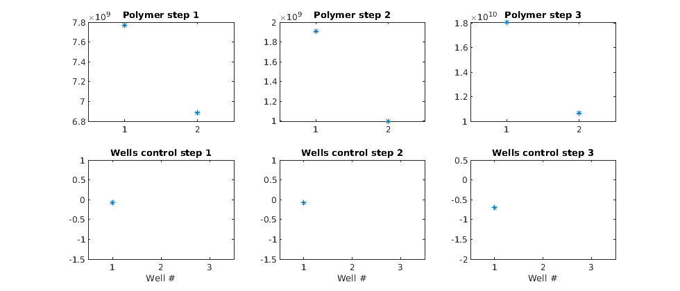
Plot the gradients¶

Plot the polymer and well gradients. Note that the second injection well, which injects less polymer, should be matched with the first to maximize the value. If we were to employ this example in an optimization loop using some external algorithm, we could optimize the polymer injection rate with regards to the total reservoir value.

figure(gcf); clf;
ng = numel(adjointGradient);
for i = 1:ng
    subplot(2,ng,i)
    plot(adjointGradient{i}(1:2), '*');
    title(['Polymer step ' num2str(i) ])
    set(gca, 'xtick', [1;2], 'xlim', [0.5;2.5]);
    axis 'auto y'
    subplot(2,ng,i+3)
    plot(adjointGradient{i}(3:end), '*'); axis tight
    title(['Wells control step ' num2str(i) ])
    set(gca, 'xtick', [1;2;3], 'xlim', [0.5; 3.5]);
    axis 'auto y'
    xlabel('Well #')
end

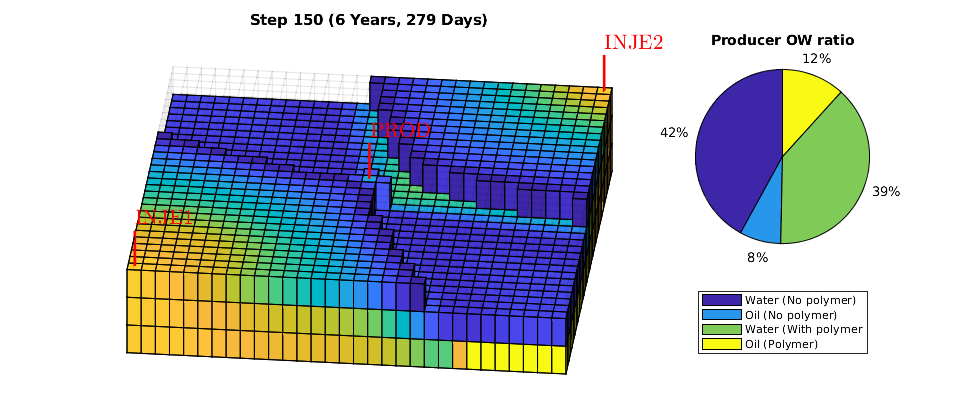
_images/adjointWithPolymerExample_05.png

Animation of simulation results¶

We animate the computed solutions. The animation shows all cells with water saturation exceeding the residual saturation, as well as a pie chart that shows the oil/water ratio in the producer with and without polymer injection in a single chart.

W = schedule.control(1).W;
ph = nan;
figure(gcf); clf
nDigits = floor(log10(numel(statesPolymer) - 1)) + 1;
subplot(1,3,[1 2])
plotGrid(G, 'facea', 0,'edgea', .05, 'edgec', 'k'); plotWell(G,W);
axis tight off, view(6,60), hs = [];
for i = 1 : numel(statesPolymer) - 1,
    injp  = wellSolsPolymer{i}(3);
    injow = wellSolsOW{i}(3);
    state = statesPolymer{i + 1};

    subplot(1, 3, 3), cla
    rates = injp.sign .* [injow.qWs, injow.qOs injp.qWs, injp.qOs];

    if ishandle(ph)
        delete(ph)
        ph = pie(rates./sum(rates));
    else
        ph = pie(rates./sum(rates));
        legend('Water (No polymer)', 'Oil (No polymer)', ...
               'Water (With polymer', 'Oil (Polymer)',   ...
               'Location', 'SouthOutside')
        title('Producer OW ratio'),
    end
    subplot(1, 3, [1 2]), delete(hs);
    hs = plotCellData(G,state.s(:,1),state.s(:,1)>.101);
    title(sprintf('Step %0*d (%s)', nDigits, i, formatTimeRange(cumt(i))));
    drawnow;
end

_images/adjointWithPolymerExample_06.png

If you have a powerful computer, you can replace the cell plot by a simple volume renderer by uncommenting the corresponding lines.

%{
clf,
plotGrid(G,'facea', 0,'edgea', .05, 'edgec', 'k'); plotWell(G,W);
axis tight off, view(6,60)
for i=1:numel(statesPolymer)-1
    cla
    state = statesPolymer{i + 1};
    plotGrid(G, 'facea', 0,'edgea', .05, 'edgec', 'k');
    plotGridVolumes(G, state.s(:,2), 'cmap', @copper, 'N', 10)
    plotGridVolumes(G, state.s(:,1), 'cmap', @winter, 'N', 10)
    plotGridVolumes(G, state.c,      'cmap', @autumn, 'N', 10)
    plotWell(G,W);
    title(sprintf('Step %0*d (%s)', nDigits, i, formatTimeRange(cumt(i))));
    drawnow
end
%}

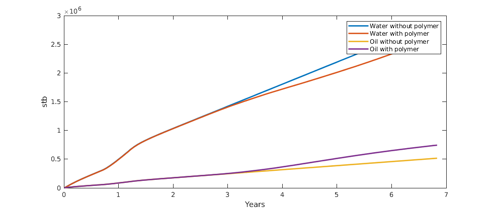
Plot the accumulated water and oil production for both cases¶

We concat the well solutions and plot the accumulated producer rates for both the polymer and the non-polymer run. The result shows that the polymer injection both gives more produced oil and less produced water and hence is a feasible stategy in this particular example.

figure(gcf); clf;
wspoly = vertcat(wellSolsPolymer{:});
wsow = vertcat(wellSolsOW{:});

data = -([ [wsow(:,3).qWs]   ; ...
           [wspoly(:,3).qWs] ; ...
           [wsow(:,3).qOs]   ; ...
           [wspoly(:,3).qOs] ] .');
data = bsxfun(@times, data, schedule.step.val);

plot(convertTo(cumt, year), cumsum(convertTo(data, stb)),'LineWidth',2);
legend({'Water without polymer', 'Water with polymer', ...
        'Oil without polymer', 'Oil with polymer'}, 'Location', 'NorthEast');
ylabel('stb');
xlabel('Years');

_images/adjointWithPolymerExample_07.png

Copyright notice¶

<html>
% <p><font size="-1

% 2D Three-Phase Polymer Injection Case
%
% This example contains a simple 4000 m-by-200 m-by-125 m reservoir
% described on 20-by-1-by-5 uniform Cartesian grid. One injection well is
% located in the bottom two layers and one production well is located in
% the top two layers. Hydrostatic equilibration is used for initialization.
%
% The polymer injection schedule follows a typical polymer waterflooding
% strategy. The flooding process begins with primary waterflooding for 1260
% days, followed by a polymer slug injected over 1700 days, and then
% switching back to water injection. The injection well is under rate
% control with target rate 1000 m3/day and upper limit of 450 bar on the
% bottom-hole pressure (bhp), whereas the production well is under pressure
% control with target bottom-home pressure 260 bar.

mrstModule add ad-core ad-blackoil ad-eor ad-props ...
               deckformat mrst-gui

Set up model and initial conditions¶

Generated from blackoilpolymerTutorial2D.m

The data required for the example If the data does not exist locally, download it automatically The following are all the files needed for this tutorial The first two files are the data for a simulation with shear-thinning effect. The second two fils are the data for a simulation without shear effect. The last two are the reference results from Eclipse.

fname = {'BOPOLYMER.DATA', ...
         'POLY.inc', ...
         'BOPOLYMER_NOSHEAR.DATA', ...
         'POLY_NOSHEAR.inc', ...
         'smry.mat', ...
         'smry_noshear.mat'};
files = fullfile(getDatasetPath('BlackoilPolymer2D', 'download', true),...
                                fname);

% check to make sure the files are complete
e = cellfun(@(pth) exist(pth, 'file') == 2, files);

if ~all(e)
    pl = ''; if sum(e) ~= 1, pl = 's'; end
    msg = sprintf('Missing data file%s\n', pl);
    msg = [msg, sprintf('  * %s\n', fname{~e})];
    error('Dataset:Incomplete', msg);
end
gravity reset on;

% Parsing the data file with shear-thinning effect.
deck = readEclipseDeck(files{1});
% The deck is using metric system, MRST uses SI unit internally
deck = convertDeckUnits(deck);

% Construct physical model, initial state and dynamic well controls.
[state0, model, schedule] = initEclipseProblemAD(deck);

% Add polymer concentration
state0.cp   = zeros([model.G.cells.num, 1]);

% maximum polymer concentration, used to handle the polymer adsorption
state0.cpmax= zeros([model.G.cells.num, 1]);

No converter needed in section 'REGIONS'.
No converter needed in section 'SUMMARY'.
No converter needed in section 'REGIONS'.
No converter needed in section 'SUMMARY'.
Processing Cells   1 : 100 of 100 ... done (0.01 [s], 1.52e+04 cells/second)
Total 3D Geometry Processing Time = 0.007 [s]
Ordering well 1 (INJE01) with strategy "origin".
Ordering well 2 (PROD01) with strategy "origin".

Select nonlinear and linear solvers¶

% Using physically normalized residuals for non-linear convergence
% calcuation.
model.useCNVConvergence = true;

% Setting up the non-linear solver.
nonlinearsolver = NonLinearSolver();
nonlinearsolver.useRelaxation = true;

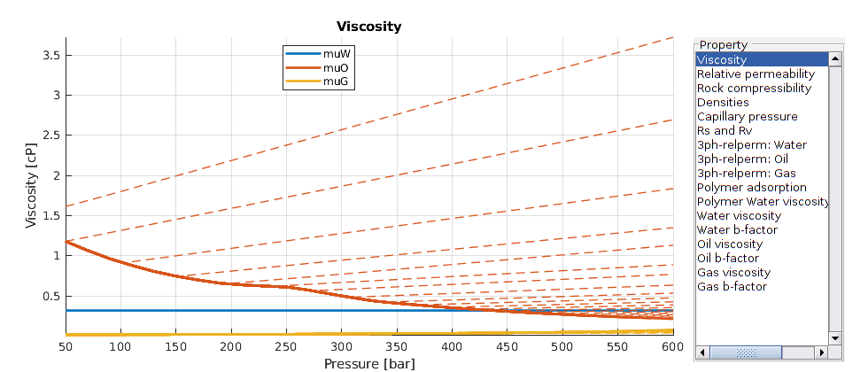
Visualize the properties of the black-oil fluid model¶

We launch the interactive viewer for the black-oil fluid model, and specify the pressure range for which the tables are given. Note that extrapolation beyond the specified values for black-oil properties can result in non-physical curves, depending on how the input was given.

inspectFluidModel(model, 'pressureRange', (50:10:600)*barsa)
example_name = 'blackoil2D';
vizPolymerModel();

_images/blackoilpolymerTutorial2D_01.png

_images/blackoilpolymerTutorial2D_02.png

_images/blackoilpolymerTutorial2D_03.png

_images/blackoilpolymerTutorial2D_04.png

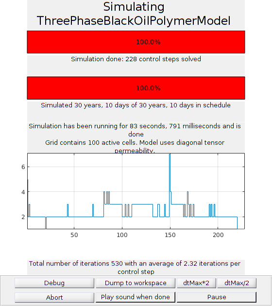
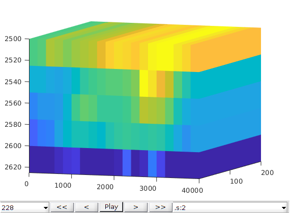
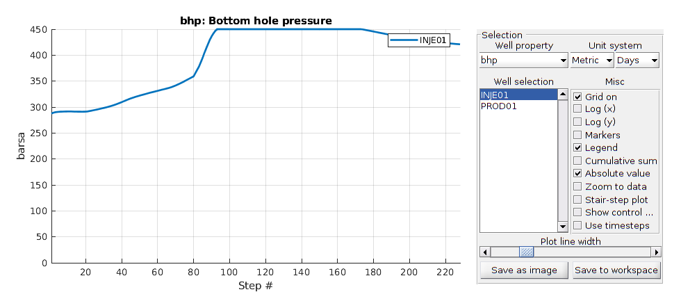
Run the schedule with plotting function¶

Once a system has been created it is trivial to run the schedule. Any options such as maximum non-linear iterations and tolerance can be set in the system struct.

% The AD-solvers allow for dyanmic plotting during the simulation process.
% We set up the following function to plot the evolution of the related
% variables (s:2 means oil saturation by default), the change of the well
% curves, and the a panel showing simulation progress. You can customize
% the function based on your own preference.
close all
fn = getPlotAfterStep(state0, model, schedule, ...
    'plotWell', true, 'plotReservoir', true, 'view', [20, 8], ...
    'field', 's:2');
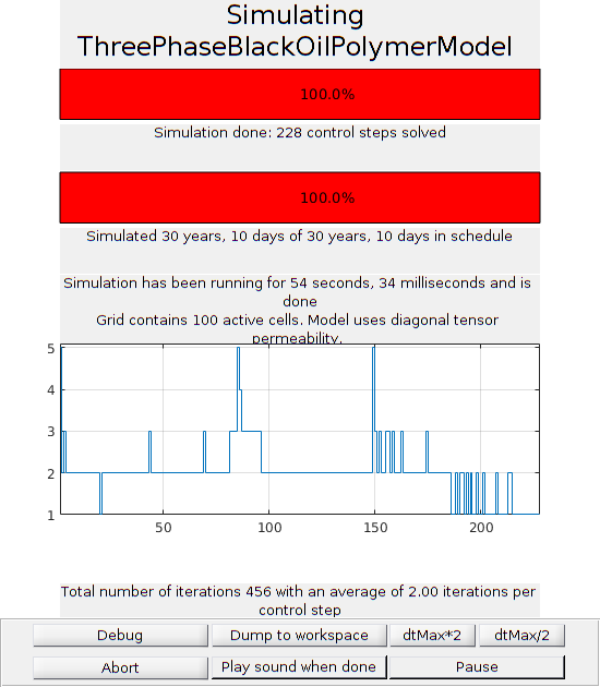
[wellSols, states, reports] = ...
    simulateScheduleAD(state0, model, schedule, ...
                    'NonLinearSolver', nonlinearsolver, 'afterStepFn', fn);

*****************************************************************
********** Starting simulation:   228 steps, 10960 days *********
*****************************************************************
Preparing model for simulation...
Model ready for simulation...
Preparing schedule for simulation...
Schedule ready for simulation...
Validating initial state...
...

_images/blackoilpolymerTutorial2D_05.png

_images/blackoilpolymerTutorial2D_06.png

_images/blackoilpolymerTutorial2D_07.png

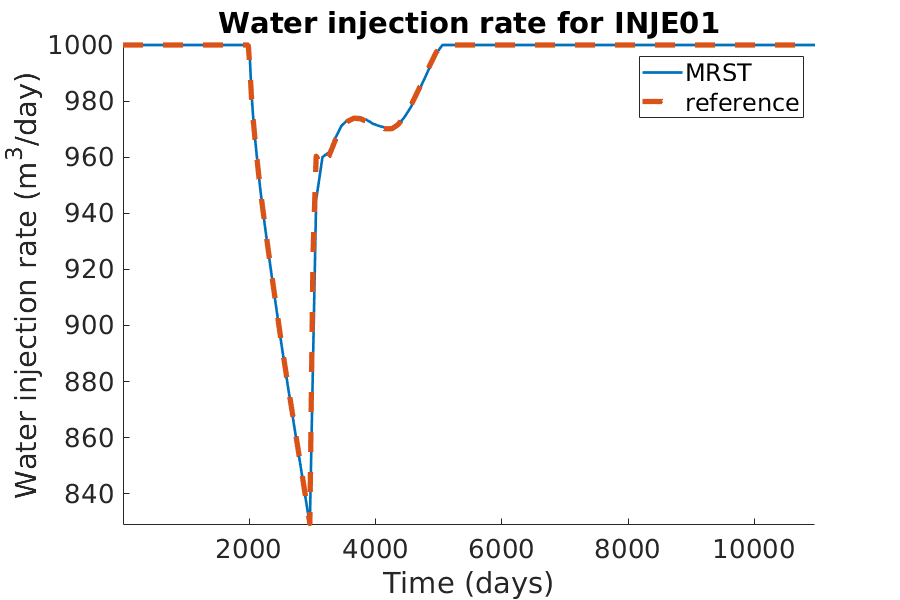
Comparing the result with reference result from commercial simualtor.¶

loading the reference result smary.mat

load (files{5});
% the time for the reference result
T_ref = smry.get(':+:+:+:+', 'TIME', ':');
% the time for the MRST result
T_mrst = convertTo(cumsum(schedule.step.val), day);

% generate a color map for plotting use.
color_map = lines(10);
color_mrst = color_map(1, :);
color_ref  = color_map(2, :);

mrstplot = @(T_mrst, data, color) plot(T_mrst, data, '-', ...
                                       'linewidth', 2, 'color', color);
referenceplot = @(T_ref, data, color) plot(T_ref, data, '--',...
                                       'linewidth', 4, 'color', color);

% Plotting the water injection rate
h = figure(); clf;
set(gca,'FontSize',20);
set(h, 'Position', [100, 100, 900, 600]);
well_name = 'INJE01';
reference = smry.get(well_name, 'WWIR', ':');
% the first value of the result of the commerical simualtor is always zero.
reference(1) = nan;
mrst = convertTo(abs(getWellOutput(wellSols, 'qWs', well_name)), ...
                                                              meter^3/day);
hold on;
mrstplot(T_mrst, mrst, color_mrst);
referenceplot(T_ref, reference, color_ref);
title(['Water injection rate for ', well_name]);
xlabel('Time (days)');
ylabel('Water injection rate (m^3/day)');
axis tight;
legend({'MRST', 'reference'})
pause(0.1);

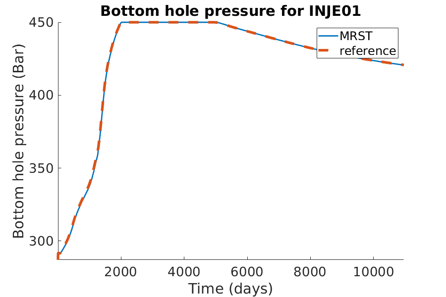
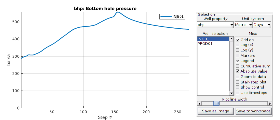
% Plotting the bhp for the injection well
h = figure(); clf;
set(gca,'FontSize',20);
set(h, 'Position', [100, 100, 900, 600]);
well_name = 'INJE01';
reference = smry.get(well_name, 'WBHP', ':');
% the first value of the result of the commerical simualtor is always zero.
reference(1) = nan;
mrst = convertTo(abs(getWellOutput(wellSols, 'bhp', well_name)), barsa);
hold on;
mrstplot(T_mrst, mrst, color_mrst);
referenceplot(T_ref, reference, color_ref);
title(['Bottom hole pressure for ', well_name]);
xlabel('Time (days)');
ylabel('Bottom hole pressure (Bar)');
axis tight;
legend({'MRST', 'reference'})
pause(0.1);

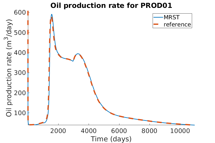
% Plotting the oil production rate
h = figure(); clf;
set(gca,'FontSize',20);
set(h, 'Position', [100, 100, 900, 600]);
well_name = 'PROD01';
reference = smry.get(well_name, 'WOPR', ':');
% the first value of the result of the commerical simualtor is always zero.
reference(1) = nan;
mrst = convertTo(abs(getWellOutput(wellSols, 'qOs', well_name)), ...
                                                              meter^3/day);
hold on;
mrstplot(T_mrst, mrst, color_mrst);
referenceplot(T_ref, reference, color_ref);
title(['Oil production rate for ', well_name]);
xlabel('Time (days)');
ylabel('Oil production rate (m^3/day)');
axis tight;
legend({'MRST', 'reference'})
pause(0.1);

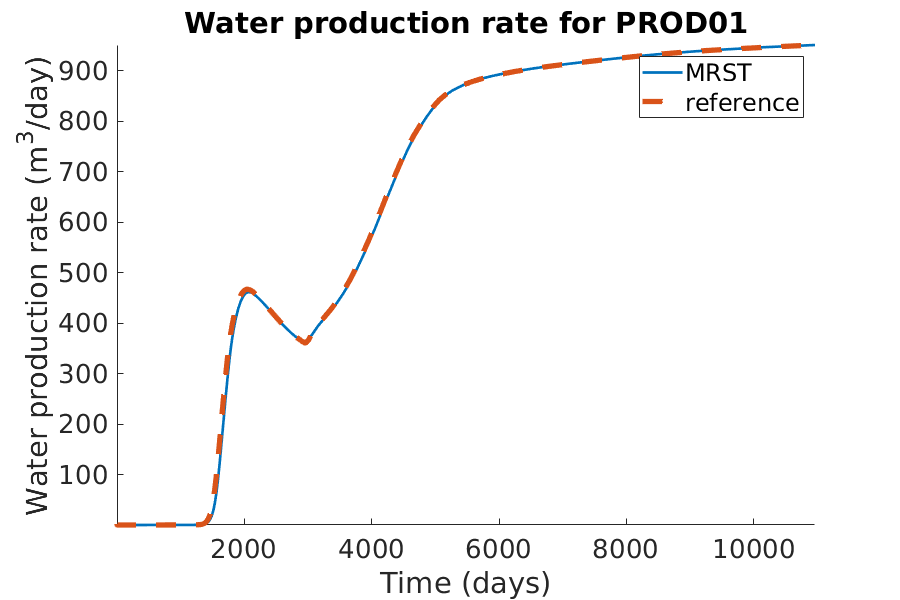
% Plotting the oil production rate
h = figure(); clf;
set(gca,'FontSize',20);
set(h, 'Position', [100, 100, 900, 600]);
well_name = 'PROD01';
reference = smry.get(well_name, 'WWPR', ':');
% the first value of the result of the commerical simualtor is always zero.
reference(1) = nan;
mrst = convertTo(abs(getWellOutput(wellSols, 'qWs', well_name)), ...
                                                             meter^3/day);
hold on;
mrstplot(T_mrst, mrst, color_mrst);
referenceplot(T_ref, reference, color_ref);
title(['Water production rate for ', well_name]);
xlabel('Time (days)');
ylabel('Water production rate (m^3/day)');
axis tight;
legend({'MRST', 'reference'})
pause(0.1);

_images/blackoilpolymerTutorial2D_08.png

_images/blackoilpolymerTutorial2D_09.png

_images/blackoilpolymerTutorial2D_10.png

_images/blackoilpolymerTutorial2D_11.png

Run the simulation without shear effect.¶

You can load the files{3} to run the simulation. Here we just modify the model directly to disable the shear effect.

close all
model.usingShear = false;

fn = getPlotAfterStep(state0, model, schedule, ...
    'plotWell', true, 'plotReservoir', true, 'view', [20, 8], ...
    'field', 's:2');
[wellSolsNoShear, statesNoShear, reportsNoShear] = ...
    simulateScheduleAD(state0, model, schedule, ...
                    'NonLinearSolver', nonlinearsolver, 'afterStepFn', fn);

*****************************************************************
********** Starting simulation:   228 steps, 10960 days *********
*****************************************************************
Preparing model for simulation...
Model ready for simulation...
Preparing schedule for simulation...
Schedule ready for simulation...
Validating initial state...
...

_images/blackoilpolymerTutorial2D_12.png

_images/blackoilpolymerTutorial2D_13.png

_images/blackoilpolymerTutorial2D_14.png

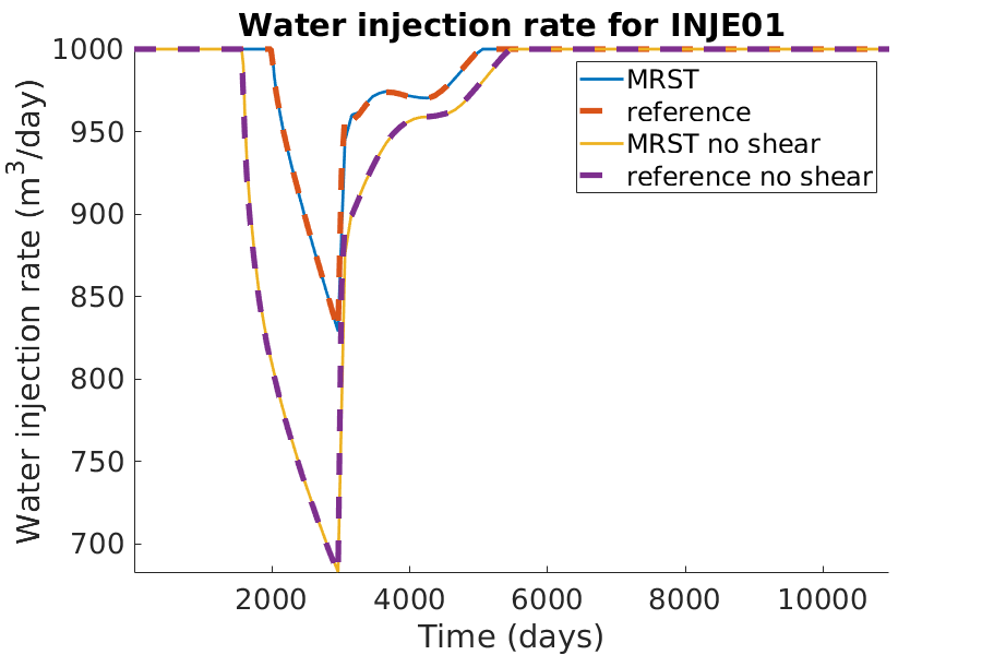
Plotting the results from two simulations and their reference results.¶

load the reference results for the non-shear case.

load (files{6});
% the time for the reference result
% since the commercial software might cut the time steps, the actually used
% schedule can be different from the previous running with shear-thinning.
T_ref_noshear = smry.get(':+:+:+:+', 'TIME', ':');

color_mrst_noshear = color_map(3, :);
color_ref_noshear = color_map(4,:);

% Plotting the water injection rate
h = figure(); clf;
set(gca,'FontSize',20);
set(h, 'Position', [100, 100, 900, 600]);
well_name = 'INJE01';
reference = smry.get(well_name, 'WWIR', ':');
reference_noshear = smry_noshear.get(well_name, 'WWIR', ':');
% the first value of the result of the commerical simualtor is always zero.
reference(1) = nan; reference_noshear(1) = nan;

mrst = convertTo(abs(getWellOutput(wellSols, 'qWs', well_name)),...
                                                        meter^3/day);
mrst_noshear = convertTo(abs(getWellOutput(wellSolsNoShear, 'qWs', ...
                                          well_name)), meter^3/day);
hold on;
mrstplot(T_mrst, mrst, color_mrst);
referenceplot(T_ref, reference, color_ref);
mrstplot(T_mrst, mrst_noshear, color_mrst_noshear);
referenceplot(T_ref_noshear, reference_noshear, color_ref_noshear);
title(['Water injection rate for ', well_name]);
xlabel('Time (days)');
ylabel('Water injection rate (m^3/day)');
axis tight;
legend({'MRST', 'reference', 'MRST no shear', 'reference no shear'})
pause(0.1);


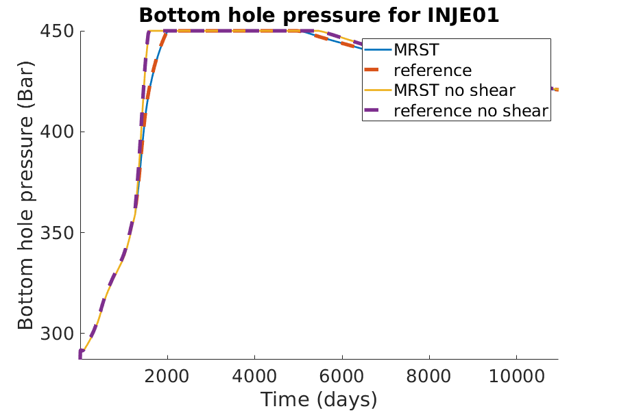
% Plotting the bhp for the injection well
h = figure(); clf;
set(gca,'FontSize',20);
set(h, 'Position', [100, 100, 900, 600]);
well_name = 'INJE01';
reference = smry.get(well_name, 'WBHP', ':');
reference_noshear = smry_noshear.get(well_name, 'WBHP', ':');
% the first value of the result of the commerical simualtor is always zero.
reference(1) = nan; reference_noshear(1) = nan;
mrst = convertTo(abs(getWellOutput(wellSols, 'bhp', well_name)), barsa);
mrst_noshear = convertTo(abs(getWellOutput(wellSolsNoShear, 'bhp', ...
                                           well_name)), barsa);
hold on;
mrstplot(T_mrst, mrst, color_mrst);
referenceplot(T_ref, reference, color_ref);
mrstplot(T_mrst, mrst_noshear, color_mrst_noshear);
referenceplot(T_ref_noshear, reference_noshear, color_ref_noshear);
title(['Bottom hole pressure for ', well_name]);
xlabel('Time (days)');
ylabel('Bottom hole pressure (Bar)');
axis tight;
legend({'MRST', 'reference', 'MRST no shear', 'reference no shear'})
pause(0.1);

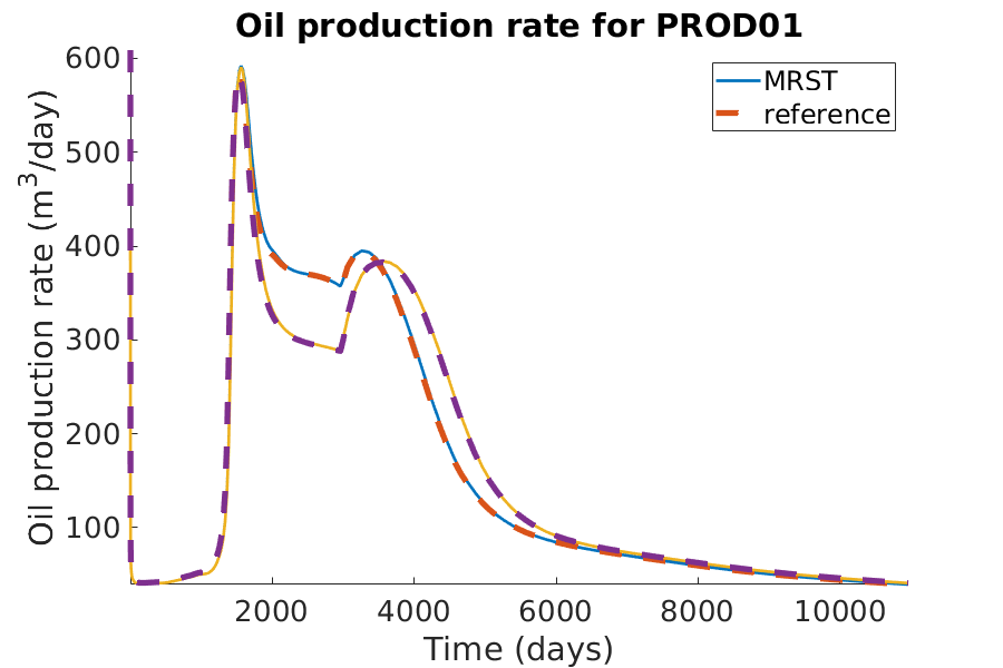
% Plotting the oil production rate
h = figure(); clf;
set(gca,'FontSize',20);
set(h, 'Position', [100, 100, 900, 600]);
well_name = 'PROD01';
reference = smry.get(well_name, 'WOPR', ':');
reference_noshear = smry_noshear.get(well_name, 'WOPR', ':');
% the first value of the result of the commerical simualtor is always zero.
reference(1) = nan; reference_noshear(1) = nan;
mrst = convertTo(abs(getWellOutput(wellSols, 'qOs', well_name)), ...
                                                          meter^3/day);
mrst_noshear = convertTo(abs(getWellOutput(wellSolsNoShear, 'qOs', ...
                                          well_name)), meter^3/day);
hold on;
mrstplot(T_mrst, mrst, color_mrst);
referenceplot(T_ref, reference, color_ref);
mrstplot(T_mrst, mrst_noshear, color_mrst_noshear);
referenceplot(T_ref_noshear, reference_noshear, color_ref_noshear);
title(['Oil production rate for ', well_name]);
xlabel('Time (days)');
ylabel('Oil production rate (m^3/day)');
axis tight;
legend({'MRST', 'reference'})
pause(0.1);

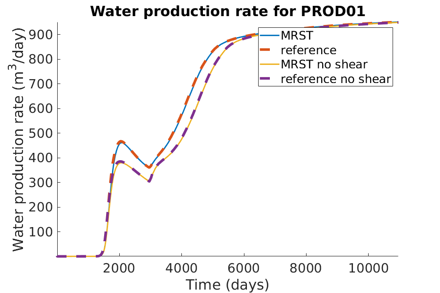
% Plotting the water production rate
h = figure(); clf;
set(gca,'FontSize',20);
set(h, 'Position', [100, 100, 900, 600]);
well_name = 'PROD01';
reference = smry.get(well_name, 'WWPR', ':');
reference_noshear = smry_noshear.get(well_name, 'WWPR', ':');
% the first value of the result of the commerical simualtor is always zero.
reference(1) = nan; reference_noshear(1) = nan;
mrst = convertTo(abs(getWellOutput(wellSols, 'qWs', well_name)), ...
                                                              meter^3/day);
mrst_noshear = convertTo(abs(getWellOutput(wellSolsNoShear, 'qWs', ...
                                          well_name)), meter^3/day);
hold on;
mrstplot(T_mrst, mrst, color_mrst);
referenceplot(T_ref, reference, color_ref);
mrstplot(T_mrst, mrst_noshear, color_mrst_noshear);
referenceplot(T_ref_noshear, reference_noshear, color_ref_noshear);
title(['Water production rate for ', well_name]);
xlabel('Time (days)');
ylabel('Water production rate (m^3/day)');
axis tight;
legend({'MRST', 'reference', 'MRST no shear', 'reference no shear'})
pause(0.1);

_images/blackoilpolymerTutorial2D_15.png

_images/blackoilpolymerTutorial2D_16.png

_images/blackoilpolymerTutorial2D_17.png

_images/blackoilpolymerTutorial2D_18.png

save resMRSTPolymer wellSols states schedule;

fprintf('The simulation has been finished! \n');

The simulation has been finished!

Copyright notice¶

<html>
% <p><font size="-1

Polymer solver with boundary conditions and sources¶

Generated from polymerBCExample.m

This example is made just to illustrate how one can setup a polymer simulation with boundary conditions and/or source.

% Required modules
mrstModule add deckformat ad-core ad-blackoil ad-eor ad-props mrst-gui

Setup case¶

% Grid, rock and fluid
deck  = readEclipseDeck('POLYMER.DATA');
deck  = convertDeckUnits(deck);
G     = initEclipseGrid(deck);
G     = computeGeometry(G);
rock  = initEclipseRock(deck);
rock  = compressRock(rock, G.cells.indexMap);
fluid = initDeckADIFluid(deck);

% Gravity
gravity on

% Initial state
state0      = initResSol(G, 100*barsa, [ .1, .9]);
state0.cp    = zeros(G.cells.num,1);
state0.cpmax = zeros(G.cells.num,1);

% Create model
model = OilWaterPolymerModel(G, rock, fluid);

% Setup some schedule
dt = 25*day;
nt = 40;
clear schedule
timesteps = repmat(dt, nt, 1);

No converter needed in section 'REGIONS'.
No converter needed in section 'SUMMARY'.
Processing Cells    1 : 2883 of 2883 ... done (0.02 [s], 1.35e+05 cells/second)
Total 3D Geometry Processing Time = 0.021 [s]

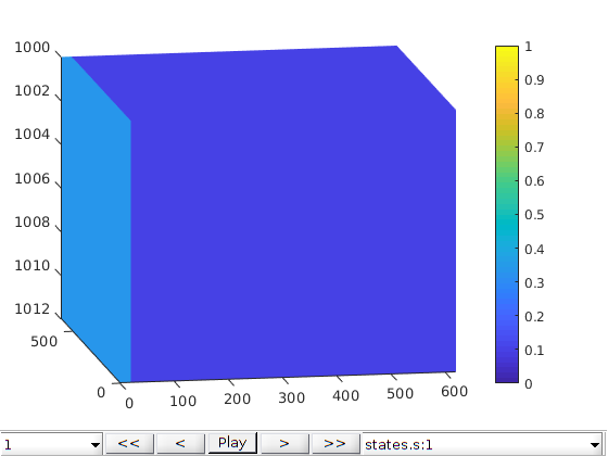
Pressure (Dirichlet) Boundary Condition¶

% Create Dirichlet boundary condition
bc = pside([], G, 'xmin', 500*barsa, 'sat', [1 0]);
bc = pside(bc, G, 'xmax', 100*barsa, 'sat', [0 0]);
bc.cp = 4.*ones(size(bc.sat,1), 1);

schedule = simpleSchedule(timesteps, 'bc', bc);

% Simulate
[~, states] = simulateScheduleAD(state0, model, schedule);

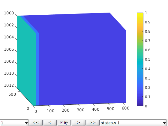
% Plot results in GUI
figure;
plotToolbar(G, states,'field', 's:1','lockCaxis',true);
view([-10, 14]);
axis tight;
colorbar; caxis([0 1]);

*****************************************************************
********** Starting simulation:    40 steps,  1000 days *********
*****************************************************************
Preparing model for simulation...
Model ready for simulation...
Preparing schedule for simulation...
Schedule ready for simulation...
Validating initial state...
...

Flux (Neumann) Boundary Condition¶

% Create Neumann boundary condition
bc = fluxside([], G, 'xmin',  0.005, 'sat', [1 0]);
bc = fluxside(bc, G, 'xmax', -0.005, 'sat', [0 0]);
bc.cp = 4.*ones(size(bc.sat,1), 1);
schedule = simpleSchedule(timesteps, 'bc', bc);

% Simulate
[~, states] = simulateScheduleAD(state0, model, schedule);

% Plot results in GUI
figure;
plotToolbar(G, states,'field', 's:1','lockCaxis',true);
view([-10, 14]);
axis tight;
colorbar; caxis([0 1]);

*****************************************************************
********** Starting simulation:    40 steps,  1000 days *********
*****************************************************************
Preparing model for simulation...
Model ready for simulation...
Preparing schedule for simulation...
Schedule ready for simulation...
Validating initial state...
...

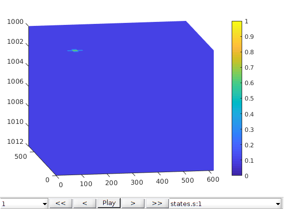
Source¶

% Create source
ijk = gridLogicalIndices(G);
srcCells = find(ijk{1}==5  & ijk{2}==5  & ijk{3}==2);
snkCells = find(ijk{1}==26 & ijk{2}==26 & ijk{3}==2);
srcVals  = 0.001.*ones(numel(srcCells),1);
src = addSource( [], srcCells,  srcVals, 'sat', [1 0]);
src = addSource(src, snkCells, -srcVals, 'sat', [0 0]);
src.cp = 4.*ones(size(src.sat,1), 1);
schedule = simpleSchedule(timesteps, 'src', src);

% Simulate
[~, states] = simulateScheduleAD(state0, model, schedule);

% Plot results in GUI
figure;
plotToolbar(G, states,'field', 's:1','lockCaxis',true);
view([-10, 14]);
axis tight;
colorbar; caxis([0 1]);

*****************************************************************
********** Starting simulation:    40 steps,  1000 days *********
*****************************************************************
Preparing model for simulation...
Model ready for simulation...
Preparing schedule for simulation...
Schedule ready for simulation...
Validating initial state...
...

Copyright notice¶

<html>
% <p><font size="-1

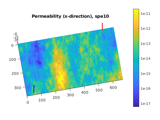
Black-Oil Polymer System for a Layer of the SPE10 Model¶

Generated from spe10PolymerExample.m

mrstModule add ad-core ad-blackoil ad-eor ad-props deckformat mrst-gui spe10

Use setupSPE10_AD to Fetch the SPE10 model¶

We pick up only one layer

layers = 35;
[~, model, ~] = setupSPE10_AD('layers', layers);
% We recover the grid and rock properties from the model
G = model.G;
rock = model.rock;

Defaulting reference depth to top of formation for well P1. Please specify 'refDepth' optional argument to 'addWell' if you require bhp at a specific depth.
Defaulting reference depth to top of formation for well P2. Please specify 'refDepth' optional argument to 'addWell' if you require bhp at a specific depth.
Defaulting reference depth to top of formation for well P3. Please specify 'refDepth' optional argument to 'addWell' if you require bhp at a specific depth.
Defaulting reference depth to top of formation for well P4. Please specify 'refDepth' optional argument to 'addWell' if you require bhp at a specific depth.
Defaulting reference depth to top of formation for well I1. Please specify 'refDepth' optional argument to 'addWell' if you require bhp at a specific depth.

Fluid Properties¶

We use the same blackoil properties as in the 2D case.

fname = {'BOPOLYMER.DATA', ...
         'POLY.inc', ...
         'BOPOLYMER_NOSHEAR.DATA', ...
         'POLY_NOSHEAR.inc', ...
        };
files = fullfile(getDatasetPath('BlackoilPolymer2D', 'download', true), fname);

% check to make sure the files are complete
e = cellfun(@(pth) exist(pth, 'file') == 2, files);

if ~all(e),
    pl = ''; if sum(e) ~= 1, pl = 's'; end
    msg = sprintf('Missing data file%s\n', pl);
    msg = [msg, sprintf('  * %s\n', fname{~e})];
    error('Dataset:Incomplete', msg);
end


% Parsing the data file with shear-thinning effect.
deck = readEclipseDeck(files{1});
% The deck is using metric system, MRST uses SI unit internally
deck = convertDeckUnits(deck);

% fluid properties, such as densities, viscosities, relative
% permeability, etc.
fluid = initDeckADIFluid(deck);

No converter needed in section 'REGIONS'.
No converter needed in section 'SUMMARY'.

Constructing the physical model used for this simulation¶

Here, we use three phase blackoil-polymer model

model = ThreePhaseBlackOilPolymerModel(G, rock, fluid);
model.disgas = true;
model.vapoil = true;

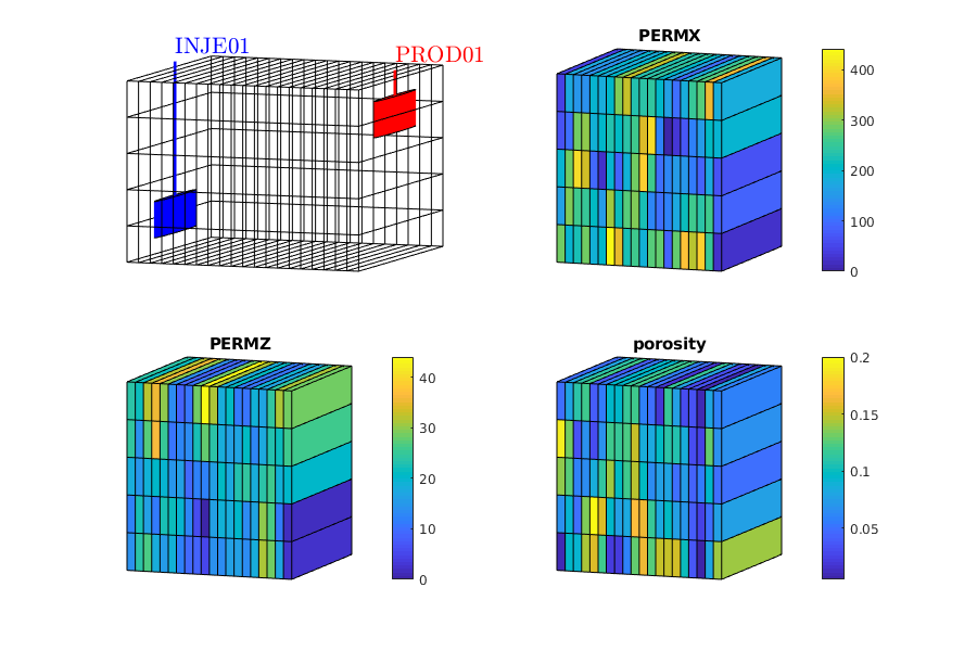
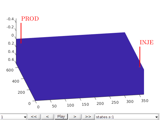
Define the Wells¶

The wells are set to operate with a high rate and no pressure limit. Hence, the pressure will rise to far above what can be used in real operational settings. However, the main point of the example is to force flow through large parts of the heterogeneous reservoir and observe the evolution of the displacement fronts.

injeIJ = [59  17];        % Location of injection well
prodIJ = [ 2 194];        % Location of production well
rate   = 2*meter^3/day;   % Injection rate
bhp    = 200*barsa;       % Pressure at production well
nz     = G.cartDims(3);

W = [];
% Set up injection well (rate control)
% The polymer injection concentration is set later, see below
W = verticalWell(W, G, rock, injeIJ(1), injeIJ(2), 1:nz, ...
                 'Type'   , 'rate', ...
                 'Val'    , rate, ...
                 'Radius' , 0.1, ...
                 'Comp_i' , [1, 0, 0], ...
                 'cp'     , 0, ...
                 'name'   , 'INJE', ...
                 'Sign'   , 1);
% Set up production well (pressure control)
bhpProd = 100*barsa;
W = verticalWell(W, G, rock, prodIJ(1), prodIJ(2), 1:nz, ...
                 'Type'   , 'bhp', ...
                 'Val'    , bhpProd, ...
                 'Radius' , 0.1, ...
                 'Comp_i' , [0, 0, 1], ...
                 'cp'     , 0, ...
                 'name'   , 'PROD', ...
                 'Sign'   , -1);

Defaulting reference depth to top of formation for well INJE. Please specify 'refDepth' optional argument to 'addWell' if you require bhp at a specific depth.
Defaulting reference depth to top of formation for well PROD. Please specify 'refDepth' optional argument to 'addWell' if you require bhp at a specific depth.

Setup the Schedule¶

We simulate the formation of a polymer plug. Three periods: 1) water only (100 days) 2) water + polymer (50 days) 3) water only (150 days) We set up a short schedule so that the computations do not take to much time in this example.

control(1).W = W;
[W([W.sign] > 0).cp] = 2*kilogram/meter^3;
control(2).W = W;

polyinj_stop_time  = 150*day;
end_time           = 300*day;

dt = 10*day;

val1 = linspace(0, polyinj_stop_time, round(polyinj_stop_time/dt));
val2 = linspace(polyinj_stop_time, end_time, round((end_time -polyinj_stop_time)/dt));
step.val     = [diff(val1'); ...
                diff(val2')];
step.control = [2*ones(numel(val1)-1, 1); ...
                1*ones(numel(val2)-1, 1)];
schedule.step    = step;
schedule.control = control;

% Refine schedule at start.
schedule = refineSchedule(0, day*ones(10, 1), schedule);

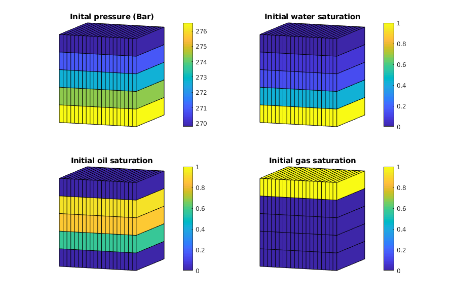
Setup the initial state¶

nc = G.cells.num;
state0.pressure = ones(nc, 1)*bhpProd;
state0.s        = ones(nc, 1)*[0, 0, 1];
state0.rs       = 0.5*fluid.rsSat(state0.pressure);
state0.rv       = zeros(nc, 1);
state0.cp       = zeros(G.cells.num, 1);
state0.cpmax    = state0.cp;

visualize the model properties¶

example_name = 'spe10';
vizPolymerModel();

Run the simulation¶

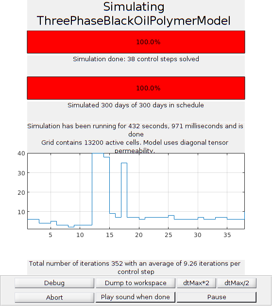
Generates function handle that set up dynamic plotting for the simulation

fn = getPlotAfterStep(state0, model, schedule, 'plotWell', true, ...
                      'plotReservoir', false);
[wellSols, states] = simulateScheduleAD(state0, model, schedule, 'afterStepFn', ...
                                        fn);

*****************************************************************
********** Starting simulation:    38 steps,   300 days *********
*****************************************************************
Preparing model for simulation...
Model ready for simulation...
Preparing schedule for simulation...
Schedule ready for simulation...
Validating initial state...
...

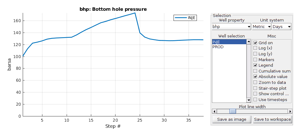
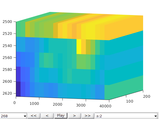
Inspect the results¶

figure, plotToolbar(G, states,'field','s:1'); plotWell(G,W,'height',.5);
view(-10,40); axis tight

Copyright notice¶

<html>
% <p><font size="-1

2D Tutorial For ad Black-Oil-Surfactant system¶

Generated from BOtutorialSurfactant2D.m

The input data is read from a deck using Eclipse format (BOSURFACTANT2D.DATA). The surfactant properties (see file surfact.inc) are taken from SPE paper 145036. Surfactant is added to water in order to decrease the surface tension so that, in particular, the residual oil is mobilized. See more detail about the modeling equations in ad-eor/docs In this example, water and surfactant are injected at the left-hand side and oil is produced at the right-hand side at a given pressure. In a first period, only water is injected. Then, for a second period, surfactant is added to the water.

We load the necessary modules¶

clear
clc
mrstModule add ad-core ad-blackoil ad-eor ad-props deckformat mrst-gui

We load the input data and setup the grid, rock and fluid structures¶

current_dir = fileparts(mfilename('fullpath'));
fn = fullfile(current_dir, 'Test_BOSURFACTANT2D.DATA');

gravity on

deck = readEclipseDeck(fn);
deck = convertDeckUnits(deck);

fluid = initDeckADIFluid(deck);
G = initEclipseGrid(deck);
G = computeGeometry(G);
rock  = initEclipseRock(deck);
rock  = compressRock(rock, G.cells.indexMap);

No converter needed in section 'REGIONS'.
No converter needed in section 'SUMMARY'.
Processing Cells   1 : 100 of 100 ... done (0.00 [s], 5.06e+04 cells/second)
Total 3D Geometry Processing Time = 0.002 [s]

Set up the model¶

The model object contains the grid, the fluid and rock properties and the modeling equations. See simulatorWorkFlowExample.

model = ThreePhaseBlackOilSurfactantModel(G, rock, fluid, ...
                                                  'inputdata', deck, ...
                                                  'extraStateOutput', true);

Convert the deck schedule into a MRST schedule by parsing the wells¶

schedule = convertDeckScheduleToMRST(model, deck);
state0 = initStateDeck(model,deck);
state0.cs    = zeros(G.cells.num, 1);
state0.csmax = state0.cs;

Ordering well 1 (INJE01) with strategy "origin".
Ordering well 2 (PROD01) with strategy "origin".

Run the schedule and set up the initial state¶

We use the function simulateScheduleAD to run the simulation Options such as maximum non-linear iterations and tolerance can be set in the system struct.

fn = getPlotAfterStep(state0, model, schedule, 'plotWell', true, ...
                      'plotReservoir', true, 'view', [20, 8], ...
                      'field', 's:2');

[wellSolsSurfactant, statesSurfactant, reportSurfactant] = simulateScheduleAD(state0, model, schedule, 'afterStepFn', fn);

% we use schedulew to run the three phase black oil water flooding simulation.
scheduleW = schedule;
scheduleW.control(1).W(1).cs = 0;
scheduleW.control(1).W(2).cs = 0;
scheduleW.control(2).W(1).cs = 0;
scheduleW.control(2).W(2).cs = 0;
scheduleW.control(3).W(1).cs = 0;
scheduleW.control(3).W(2).cs = 0;
[wellSolsW, statesW, reportW] = simulateScheduleAD(state0, model, scheduleW, 'afterStepFn', fn);

*****************************************************************
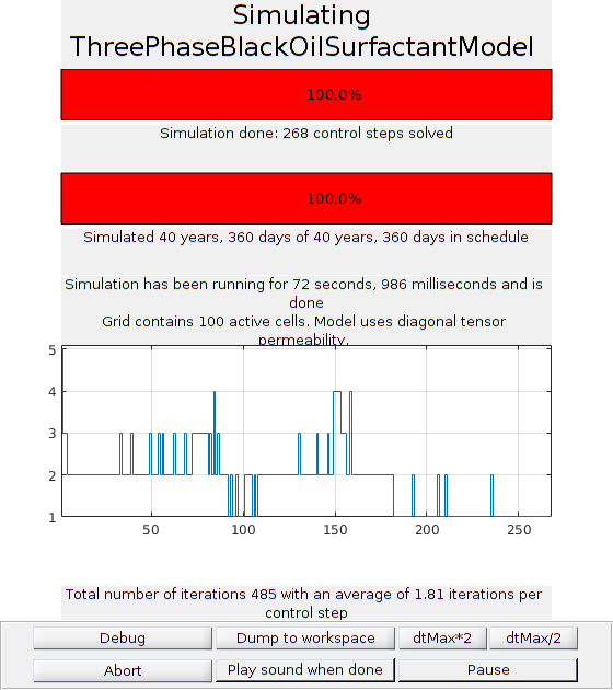
********** Starting simulation:   268 steps, 14960 days *********
*****************************************************************
Preparing model for simulation...
Model ready for simulation...
Preparing schedule for simulation...
Schedule ready for simulation...
Validating initial state...
...

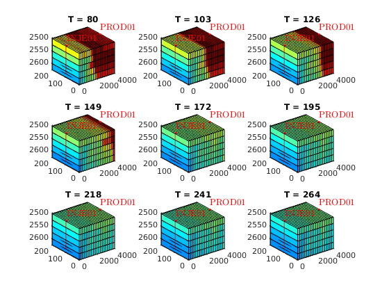
Plot cell oil saturation in different tsteps of water flooding and surfactant flooding¶

T = (80:23:268);

% Plot cell oil saturation in different tsteps of pure water flooding
sOmin = min( cellfun(@(x)min(x.s(:,2)), statesW) );
sOmax = max( cellfun(@(x)max(x.s(:,2)), statesW) );
figure
for i = 1 : length(T)
    subplot(3,3,i)
    plotCellData(model.G, statesW{T(i)}.s(:,2))
    plotWell(model.G, schedule.control(1).W, 'fontsize', 10)
    axis tight
    colormap(jet)
    view(3)
    caxis([sOmin, sOmax])
    title(['T = ', num2str(T(i))])
end
set(gcf, 'name', 'Oil saturation for water flooding')


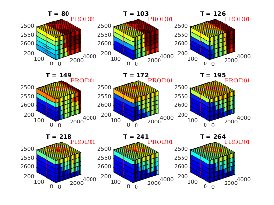
% Plot cell oil saturation in different tsteps of surfactant flooding
sOmin = min( cellfun(@(x)min(x.s(:,2)), statesSurfactant) );
sOmax = max( cellfun(@(x)max(x.s(:,2)), statesSurfactant) );
figure
for i = 1 : length(T)
    subplot(3,3,i)
    plotCellData(model.G, statesSurfactant{T(i)}.s(:,2))
    plotWell(model.G, schedule.control(1).W, 'fontsize', 10)
    axis tight
    colormap(jet)
    view(3)
    caxis([sOmin, sOmax])
    title(['T = ', num2str(T(i))])
end
set(gcf, 'name', 'Oil saturation for surfactant flooding');

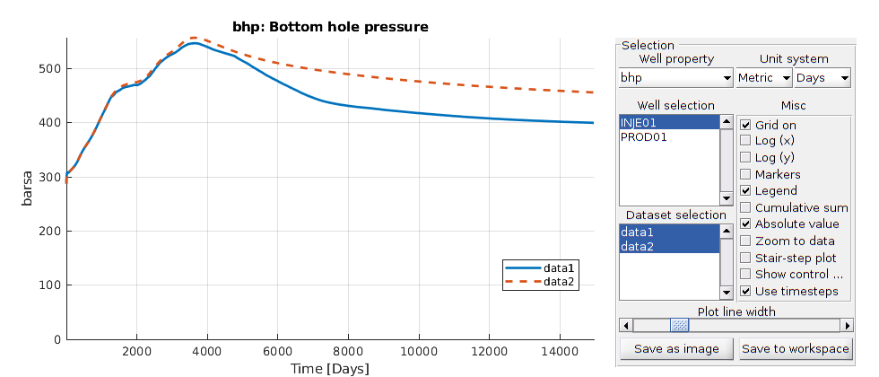
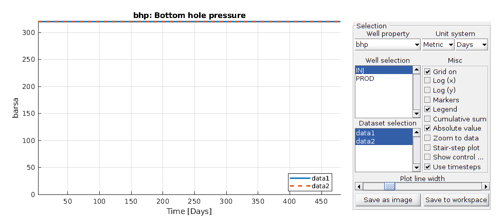
Plot well solutions¶

The orange line denotes pure water flooding while the blue line denotes surfactant flooing

plotWellSols({wellSolsSurfactant, wellSolsW}, cumsum(schedule.step.val))

Copyright notice¶

<html>
% <p><font size="-1

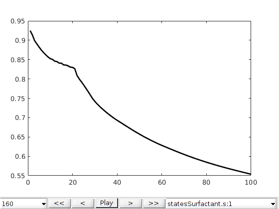
1D Tutorial For a Oil-Water-Surfactant system¶

Generated from tutorialSurfactant1D.m

The input data is read from a deck using Eclipse format (SURFACTANT1D.DATA). The surfactant property (see file surfact.inc) are taken from SPE paper 145036. Surfactant is added to water in order to decrease the surface tension so that, in particular, the residual oil is mobilized. See more detail about the modeling equations in ad-eor/docs In this example, water and surfactant are injected at the left-hand side and oil is produced at the right-hand side at a given pressure. In a first period, only water is injected. Then, for a second period, surfactant is added to the water.

We load the necessary modules¶

mrstModule add ad-core ad-blackoil ad-eor ad-props deckformat mrst-gui

We load the input data and setup the grid, rock and fluid structures¶

current_dir = fileparts(mfilename('fullpath'));
fn = fullfile(current_dir, 'SURFACTANT1D.DATA');
gravity off

deck = readEclipseDeck(fn);
deck = convertDeckUnits(deck);

fluid = initDeckADIFluid(deck);
G = initEclipseGrid(deck);
G = computeGeometry(G);
rock  = initEclipseRock(deck);
rock  = compressRock(rock, G.cells.indexMap);

No converter needed in section 'REGIONS'.
No converter needed in section 'SUMMARY'.
Processing Cells   1 : 100 of 100 ... done (0.00 [s], 2.33e+04 cells/second)
Total 3D Geometry Processing Time = 0.004 [s]

Set up the initial state¶

Constant pressure, residual water saturation, no surfactant

nc = G.cells.num;
state0 = initResSol(G, 280*barsa, [ .2, .8]); % residual water saturation is 0.2
state0.cs    = zeros(G.cells.num, 1);
state0.csmax = state0.cs;

Set up the model¶

The model object contains the grid, the fluid and rock properties and the modeling equations. See simulatorWorkFlowExample.

model = OilWaterSurfactantModel(G, rock, fluid, ...
                                                  'inputdata', deck, ...
                                                  'extraStateOutput', true);

Convert the deck schedule into a MRST schedule by parsing the wells¶

schedule = convertDeckScheduleToMRST(model, deck);

Ordering well 1 (INJ) with strategy "origin".
Ordering well 2 (PROD) with strategy "origin".

Run the schedule¶

We use the function simulateScheduleAD to run the simulation Options such as maximum non-linear iterations and tolerance can be set in the system struct.

[wellSolsSurfactant, statesSurfactant] = simulateScheduleAD(state0, model, ...
                                                  schedule);

scheduleOW = schedule;
scheduleOW.control(2).W(1).cs = 0;
scheduleOW.control(2).W(2).cs = 0;

[wellSolsOW, statesOW] = simulateScheduleAD(state0, model, ...
                                                  scheduleOW);

figure()
plotToolbar(G, statesSurfactant, 'startplayback', true, 'plot1d', true, 'field', 's:1');

plotWellSols({wellSolsSurfactant,wellSolsOW},cumsum(schedule.step.val));

*****************************************************************
********** Starting simulation:   160 steps,   480 days *********
*****************************************************************
Preparing model for simulation...
Model ready for simulation...
Preparing schedule for simulation...
Schedule ready for simulation...
Validating initial state...
...

Copyright notice¶

<html>
% <p><font size="-1

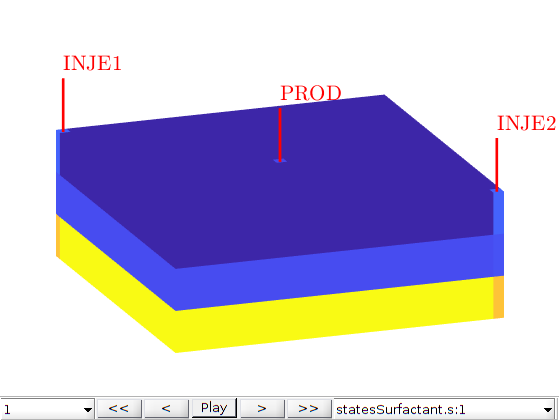
Tutorial for a simple 3D case of a oil-water-surfactant system¶

Generated from tutorialSurfactant3D.m

This example contains a

fine grid containing two injectors in opposite corners and one producer in the middle of the domain. All wells are completed in the top layers of cells.

The schedule being used contains first a period of injection with surfactant, followed by a water flooding phase without surfactant. Finally, the water rate is reduced for the final time steps. The data is read from deck (SURFACTANT3D.DATA)

mrstModule add ad-core ad-blackoil ad-eor ad-props deckformat mrst-gui

We load the input data and setup the grid, rock and fluid structures¶

current_dir = fileparts(mfilename('fullpath'));
fn = fullfile(current_dir, 'SURFACTANT3D.DATA');
gravity on

deck = readEclipseDeck(fn);
deck = convertDeckUnits(deck);

fluid = initDeckADIFluid(deck);
G = initEclipseGrid(deck);
G = computeGeometry(G);
rock  = initEclipseRock(deck);
rock  = compressRock(rock, G.cells.indexMap);

No converter needed in section 'REGIONS'.
No converter needed in section 'SUMMARY'.
Processing Cells    1 : 2883 of 2883 ... done (0.03 [s], 1.11e+05 cells/second)
Total 3D Geometry Processing Time = 0.026 [s]

Set up the initial state¶

We want a layer of oil on top of the reservoir and water on the bottom. To do this, we alter the initial state based on the logical height of each cell. Initially, the pressure is constant and the surfactant concentration is zero.

ijk = gridLogicalIndices(G);

state0 = initResSol(G, 300*barsa, [ .9, .1]);
state0.s(ijk{3} == 1, 2) = .9;
state0.s(ijk{3} == 2, 2) = .8;

% Enforce s_w + s_o = 1;
state0.s(:,1) = 1 - state0.s(:,2);

state0.cs    = zeros(G.cells.num, 1);
state0.csmax = state0.cs;

clf
plotCellData(G, state0.s(:,2));
plotGrid(G, 'facec', 'none')
title('Oil concentration')
axis tight off
view(70, 30);
colorbar;

Set up the model¶

The model object contains the grid, the fluid and rock properties and the modeling equations. See simulatorWorkFlowExample.

model = OilWaterSurfactantModel(G, rock, fluid, 'inputdata', deck);

Setup the schedule¶

The wells and wells controls obtained from the input deck are parsed and a MRST schedule is set up.

schedule = convertDeckScheduleToMRST(model, deck);

Ordering well 1 (INJE1) with strategy "origin".
Ordering well 2 (INJE2) with strategy "origin".
Ordering well 3 (PROD) with strategy "origin".

Run the schedule¶

We use the function simulateScheduleAD to run the simulation Options such as maximum non-linear iterations and tolerance can be set in the system struct. Here, we also send a resulthandler to save the output data, see ResultHandler.

resulthandler = ResultHandler('dataDirectory', pwd, 'dataFolder', 'cache', 'cleardir', true);
[wellSolsSurfactant, statesSurfactant] = simulateScheduleAD(state0, model, ...
                                                  schedule, 'OutputHandler', ...
                                                  resulthandler);
plotToolbar(G,statesSurfactant,'field','s:1');
W = schedule.control(1).W;
view(70,30), plotWell(G, W), axis tight off

*****************************************************************
********** Starting simulation:   150 steps,   510 days *********
*****************************************************************
Preparing model for simulation...
Model ready for simulation...
Preparing schedule for simulation...
Schedule ready for simulation...
Validating initial state...
...

Copyright notice¶

<html>
% <p><font size="-1

Parameters:	state0 – State at previous times-step state – State at current time-step model – Model instance dt – time-step drivingForces – Driving forces (boundary conditions, wells, …) varargin – optional parameters
Returns:	problem – Instance of LinearizedProblem state – Updated state variable (fluxes, mobilities and more can be stored, the wellSol structure is also updated in case of control switching)

Parameters:	state0 – State at previous times-step state – State at current time-step model – Model instance dt – time-step drivingForces – Driving forces (boundary conditions, wells, …) varargin – optional parameters
Returns:	problem – Instance of LinearizedProblem state – Updated state variable (fluxes, mobilities and more can be stored, the wellSol structure is also updated in case of control switching)

Parameters:	state0 – State at previous times-step state – State at current time-step model – Model instance dt – time-step drivingForces – Driving forces (boundary conditions, wells, …) varargin – optional parameters
Returns:	problem – Instance of LinearizedProblem state – Updated state variable (fluxes, mobilities and more can be stored, the wellSol structure is also updated in case of control switching)

Parameters:	state0 – State at previous times-step state – State at current time-step model – Model instance dt – time-step drivingForces – Driving forces (boundary conditions, wells, …) varargin – optional parameters
Returns:	problem – Instance of LinearizedProblem state – Updated state variable (fluxes, mobilities and more can be stored, the wellSol structure is also updated in case of control switching)

ad-eor: Enhanced oil recovery solvers¶

Models¶

Base classes¶

Utilities¶

Examples¶

Computation of Adjoints for Polymer and Waterflooding¶

Read input file and setup basic structures¶

Set up initial reservoir state¶

Plot polymer properties¶

Set up systems¶

Run the schedule¶

Objective functions¶

Plot accumulated present value¶

Compute gradients using the adjoint formulation¶

Plot the gradients¶

Animation of simulation results¶

Plot the accumulated water and oil production for both cases¶

Copyright notice¶

Set up model and initial conditions¶

Select nonlinear and linear solvers¶

Visualize the properties of the black-oil fluid model¶

Run the schedule with plotting function¶

Comparing the result with reference result from commercial simualtor.¶

Run the simulation without shear effect.¶

Plotting the results from two simulations and their reference results.¶

Copyright notice¶

Polymer solver with boundary conditions and sources¶

Setup case¶

Pressure (Dirichlet) Boundary Condition¶

Flux (Neumann) Boundary Condition¶

Source¶

Copyright notice¶

Black-Oil Polymer System for a Layer of the SPE10 Model¶

Use setupSPE10_AD to Fetch the SPE10 model¶

Fluid Properties¶

Constructing the physical model used for this simulation¶

Define the Wells¶

Setup the Schedule¶

Setup the initial state¶

visualize the model properties¶

Run the simulation¶

Inspect the results¶

Copyright notice¶

2D Tutorial For ad Black-Oil-Surfactant system¶

We load the necessary modules¶

We load the input data and setup the grid, rock and fluid structures¶

Set up the model¶

Convert the deck schedule into a MRST schedule by parsing the wells¶

Run the schedule and set up the initial state¶

Plot cell oil saturation in different tsteps of water flooding and surfactant flooding¶

Plot well solutions¶

Copyright notice¶

1D Tutorial For a Oil-Water-Surfactant system¶

We load the necessary modules¶

We load the input data and setup the grid, rock and fluid structures¶

Set up the initial state¶

Set up the model¶

Convert the deck schedule into a MRST schedule by parsing the wells¶

Run the schedule¶

Copyright notice¶

Tutorial for a simple 3D case of a oil-water-surfactant system¶

We load the input data and setup the grid, rock and fluid structures¶

Set up the initial state¶

Set up the model¶

Setup the schedule¶

Run the schedule¶

Copyright notice¶

`ad-eor`: Enhanced oil recovery solvers¶