msmfem: Multiscale Mixed Finite-Element method for pressure
Utilities
-
Contents¶ Routines supporting the multiscale mixed FE method for the pressure equation.
- Files
- basisMatrixHybrid - Form hybrid versions of the multiscale basis function matrices. basisMatrixMixed - Form mixed versions of the multiscale basis function matrices. dynamicCoarseWeight - Compute synthetic multiscale weighting function. generateCoarseSystem - Construct coarse system component matrices from fine grid model. generateCoarseWellSystem - Construct coarse system component matrices for well contributions. solveCoarsePsysBO - Solve coarsened fine-scale well system (for Black Oil). solveIncompFlowMS - Solve coarse (multiscale) pressure system. solveIncompFlowMSSpeedUp - Solve (multiscale) pressure system assuming that some values are precomputed. speedUpMS - Precompute MsMFE basis reduction matrices in order speed up assembly unpackWellSystemComponentsMS - Extract coarse linear system components from wells. updateBasisFunc - Update basis functions in regions where the total mobility has changed
-
basisMatrixHybrid(G, CG, CS)¶ Form hybrid versions of the multiscale basis function matrices.
Synopsis:
[Bv, Phi] = basisMatrixHybrid(G, CG, CS)
Parameters: - CG (G,) – Grid and coarse grid data structures, respectively.
- CS – Linear system data structure on coarse grid as defined by function ‘generateCoarseSystem’.
Returns: - Bv – Flux-basis function matrix, B*Psi.
- Phi – Pressure-basis function matrix, Phi.
See also
basisMatrixMixed,evalBasisFunc,solveIncompFlowMS.
-
basisMatrixMixed(G, CG, CS)¶ Form mixed versions of the multiscale basis function matrices.
Synopsis:
[Bv, Phi] = basisMatrixMixed(G, CG, CS)
Parameters: - CG (G,) – Grid and coarse grid data structures, respectively.
- CS – Linear system data structure on coarse grid as defined by function ‘generateCoarseSystem’.
Returns: - Bv – Flux-basis function matrix, B*Psi.
- Phi – Pressure-basis function matrix, Phi.
See also
basisMatrixHybrid,evalBasisFunc,solveIncompFlowMS.
-
dynamicCoarseWeight(cellno, BI, ct, phi, v, dpdt)¶ Compute synthetic multiscale weighting function.
Synopsis:
theta = dynamicCoarseWeight(cellno, BI, ct, phi, v, dpdt)
Parameters: - cellno –
A map giving the global cell number of any given half-face. That is, cellno(i) is the global cell to which half-face ‘i’ is connected. Typically,
nc = G.cells.num; nf = double(G.cells.numFaces); cellno = rldecode((1 : nc) .’, nf);when ‘G’ is the grid of a reservoir model.
- BI –
Inverse mass matrix, correctly updated for effects of total mobility, such that the expression
f’ * (BI f)gives the (squared) energy norm of a function ‘f’ represented on all half faces of the model.
- ct – Total compressibility. One scalar value for each global cell in the reservoir model.
- phi – Porosity. One scalar value for each global cell in the model.
- v – Current half-face fluxes for all cells in the model.
- dpdt – An approximate time derivative of the cell pressure values. One scalar value for each cell in the grid.
Returns: theta – A theta function suitable for passing in option pair (‘BasisWeighting’,theta) to function generateCoarseSystem.
See also
- cellno –
-
generateCoarseSystem(G, rock, S, CG, mob, varargin)¶ Construct coarse system component matrices from fine grid model.
Synopsis:
CS = generateCoarseSystem(G, rock, S, CG, Lt)
CS = generateCoarseSystem(G, rock, S, CG, Lt, 'pn1', pv1, ...)
Parameters: - G – Grid structure as described by grid_structure.
- rock – Rock data structure with valid field ‘perm’. If the basis functions are to be weighted by porosity, rock must also contain a valid field ‘poro’.
- S – System struture describing the underlying fine grid model, particularly the individual cell flux inner products.
- CG – Coarse grid structure as defined by generateCoarseGrid.
- mob – Total mobility. One scalar value for each cell in the underlying (fine) model.
- 'pn'/pv –
List of ‘key’/value pairs defining optional parameters. The supported options are:
- Verbose –
- Whether or not to emit progress reports while computing basis functions. Logical. Default value dependent upon global verbose setting in function ‘mrstVerbose’.
- bc – Boundary condtion structure as defined by function
- ’addBC’. This structure accounts for all external boundary contributions to the reservoir flow. Default value: bc = [] meaning all external no-flow (homogeneous Neumann) conditions.
- src – Explicit source contributions as defined by
- function ‘addSource’. Default value: src = [] meaning no explicit sources exist in the model.
- global_inf –
- global information from fine scale solution (fineSol.faceFlux) to be used as boundary condition when calculating basis for coarse faces in the interior of the domain.
- Overlap –
- Number of fine-grid cells in each physical
direction with which to extend the supporting
domain of any given basis functions.
Using overlapping domains enables capturing more complex flow patterns, particularly for very coarse grids, at the expense of increased coupling in the resulting systems of linear equations. Non-negative integers. Default value = 0.
- BasisWeighting –
- Basis function driving source term as supported by function ‘evalBasisSource’.
- ActiveBndFaces –
- Vector of active coarse boundary faces. Default value=[] (only no-flow BC). We remark that coarse faces with prescribed fine-scale BC’s are always considered active.
Returns: CS – System structure having the following fields: - basis - Flux basis functions as generated by function
evalBasisFunc.
- basisP - Pressure basis functions as generated by function
- evalBasisFunc.
- C - C in coarse hybrid system.
- D - D in coarse hybrid system.
- sizeC - size of C (== size(CS.C))
- sizeD - size of D (== size(CS.D))
See also
computeMimeticIP,generateCoarseGrid,evalBasisFunc,mrstVerbose.
-
generateCoarseWellSystem(G, S, CG, CS, mob, rock, W, varargin)¶ Construct coarse system component matrices for well contributions.
Synopsis:
W = generateCoarseWellSystem(G, S, CG, CS, mob, rock, W)
W = generateCoarseWellSystem(G, S, CG, CS, mob, rock, W, ...
                             'pn1', pv1, ...)
Parameters: - G – Grid data structure.
- S – System structure describing the underlying fine grid model, particularly the individual cell flux inner products.
- CG – Coarse grid structure as defined by function generateCoarseGrid.
- CS – Coarse system structure as defined by function generateCoarseSystem.
- mob – Total mobility. One scalar value for each cell in the underlying (fine) model.
- rock – Rock data structure. May be empty, but must contain valid field ‘rock.perm’ if the synthetic driving source term for basis functions is ‘perm’. Similarly, if the driving source term is ‘poros’, then the rock data structure must contain a valid field ‘rock.poro’.
- W – Well structure as defined by function addWell.
- 'pn'/pv –
List of ‘key’/value pairs defining optional parameters. The supported options are:
- src – Explicit source terms in the underlying fine grid
- model which must be taken into account when
generating the basis functions. Note that basis
functions in blocks containing an explicit source
term will be generated based solely on the
explicit source. The values in ‘weight’
pertaining to such blocks will be ignored.
Must be a source data structure as defined by function ‘addSource’. Default value is [] (an empty array), meaning that no explicit sources are present in the model.
- OverlapWell –
- Number of fine grid cells by which to extend support of the well basis function about the well bore.
- OverlapBlock –
- Number of fine grid cells by which to extend support of the well basis function about the reservoir coarse block.
Returns: W – Updated well structure having new field W(i).CS defined as W(i).CS.basis : Cell array of SPARSE input vectors from which well
flux basis function matrix may be formed.
- W(i).CS.basisP: Cell array of SPARSE input vectors from which well
pressure basis function matrix may be formed.
W(i).CS.rates : Sparse matrix of well rates.
W(i).CS.C : | MS discretization matrices wrt activeFaces W(i).CS.D : /
W(i).CS.RHS.f : | Coarse well system right hand sides W(i).CS.RHS.h : /
See also
-
solveCoarsePsysBO(state, G, CG, p, rock, S, CS, fluid, p0, dt, varargin)¶ Solve coarsened fine-scale well system (for Black Oil).
Synopsis:
[xr, xw] = solveCoarsePsysBO(xr, xw, G, CG, p, rock, S, CS, ...
                             fluid, p0, dt)
[xr, xw] = solveCoarsePsysBO(xr, xw, G, CG, p, rock, S, CS, ...
                             fluid, p0, dt, 'pn1', pv1, ...)
Parameters: - xw (xr,) – Reservoir and well solution structures either properly initialized from functions ‘initResSol’ and ‘initWellSol’ respectively, or the results from a previous call to function ‘solveCoarsePsysBO’.
- CG, p (G,) – Grid, coarse grid, and cell-to-block partition vector, respectively.
- rock – Rock data structure. Must contain valid field ‘rock.perm’.
- CS (S,) – Linear system structure on fine grid (S) and coarse grid (CS) as defined by functions ‘computeMimeticIP’ and ‘generateCoarseSystem’, respectively.
- fluid – Black Oil fluid object as defined by, e.g., function ‘initBlackoilFluid’.
- p0 – Vector, length G.cells.num, of cell pressures at previous time step (not previous iteration of successive substitution algorithm).
- dt – Time step size.
Keyword Arguments: wells – Well structure as defined by functions ‘addWell’ and ‘generateCoarseWellSystem’. May be empty (i.e., W = [], default value) which is interpreted as a model without any wells.
bc – Boundary condition structure as defined by function ‘addBC’. This structure accounts for all external boundary conditions to the reservoir flow. May be empty (i.e., bc = [], default value) which is interpreted as all external no-flow (homogeneous Neumann) conditions.
src – Explicit source contributions as defined by function ‘addSource’. May be empty (i.e., src = [], default value) which is interpreted as a reservoir model without explicit sources.
LinSolve – Handle to linear system solver software to which the fully assembled system of linear equations will be passed. Assumed to support the syntax
x = LinSolve(A, b)
in order to solve a system Ax=b of linear equations. Default value: LinSolve = @mldivide (backslash).
Returns: xr, xw – Updated reservoir and well solution structures. The reservoir solution structure ‘xr’ will have added fields ‘blockPressure’ and ‘blockFlux’ corresponding to the coarse grid pressure and block fluxes, respectively.
See also
solveBlackOilWellSystem.
-
solveIncompFlowMS(state, G, CG, p, S, CS, fluid, varargin)¶ Solve coarse (multiscale) pressure system.
Synopsis:
state = solveIncompFlowMS(state, G, CG, p, S, CS, fluid)
state = solveIncompFlowMS(state, G, CG, p, S, CS, fluid, ...
                          'pn1', pv1, ...)
Description:
This function assembles and solves a (block) system of linear equations defining interface fluxes and cell and interface pressures at the next time step in a sequential splitting scheme for the reservoir simulation problem defined by Darcy’s law and a given set of external influences (wells, sources, and boundary conditions).
Parameters: - state – Reservoir and well solution structure either properly initialized from functions ‘initResSol’ and ‘initWellSol’ respectively, or the results from a previous call to function ‘solveIncompFlowMS’ and, possibly, a transport solver such as function ‘implicitTransport’.
- CG, p (G,) – Grid, coarse grid, and cell-to-block partition vector, respectively.
- CS (S,) – Linear system structure on fine grid (S) and coarse grid (CS) as defined by functions ‘computeMimeticIP’ and ‘generateCoarseSystem’, respectively.
- fluid – Fluid object as defined by function ‘initSimpleFluid’.
Keyword Arguments: wells – well linear system structure (W) as defined by functions ‘addWell’, ‘assembleWellSystem’, and ‘assembleCoarseWellSystem’. An empty well linear system structure (i.e., W=struct([])) is supported. The resulting model is interpreted as not containing any well driving forces.
bc – Boundary condition structure as defined by function ‘addBC’. This structure accounts for all external boundary conditions to the reservoir flow. May be empty (i.e., bc = struct([])) which is interpreted as all external no-flow (homogeneous Neumann) conditions.
src – Explicit source contributions as defined by function ‘addSource’. May be empty (i.e., src = struct([])) which is interpreted as a reservoir model without explicit sources.
rhs – Supply system right-hand side ‘b’ directly. Overrides internally constructed system right-hand side. Must be a three-element cell array, the elements of which are correctly sized for the block system component to be replaced.
NOTE: This is a special purpose option for use by code which needs to modify the system of linear equations directly, e.g., the ‘adjoint’ code.
Solver – Which solver mode function ‘solveIncompFlowMS’ should employ in assembling and solving the block system of linear equations. String. Default value: Solver = ‘hybrid’.
- Supported values are:
- ‘hybrid’ –
- Assemble and solve hybrid system for interface pressures. System is eventually solved by Schur complement reduction and back substitution. The hybrid solver can not be employed if any of the basis functions in the coarse system were generated with a positive overlap.
- ‘mixed’ –
- Assemble and solve a mixed system for cell pressures and interface fluxes.
LinSolve – Handle to linear system solver software to which the fully assembled system of linear equations will be passed. Assumed to support the syntax
x = LinSolve(A, b)
in order to solve a system Ax=b of linear equations. Default value: LinSolve = @mldivide (backslash).
MatrixOutput – Whether or not to return the final system matrix ‘A’ to the caller of function ‘solveIncompFlowMS’. Logical. Default value: MatrixOutput = FALSE.
Returns: xr – Reservoir solution structure with new values for the fields: - cellPressure – Pressure values for all cells in the
discretised reservoir model, ‘G’.
- facePressure – Pressure values for all interfaces in the
- discretised reservoir model, ‘G’.
- cellFlux – Outgoing flux across each local interface for
- all cells in the model.
- faceFlux – Flux across global interfaces corresponding to
- the rows of ‘G.faces.neighbors’.
- A – System matrix. Only returned if specifically
- requested by setting option ‘MatrixOutput’.
xw – Well solution structure array, one element for each well in the model, with new values for the fields:
- flux – Perforation fluxes through all perforations for
- corresponding well. The fluxes are interpreted as injection fluxes, meaning positive values correspond to injection into reservoir while negative values mean production/extraction out of reservoir.
- pressure – Well pressure.
Note
If there are no external influences, i.e., if all of the structures ‘W’, ‘bc’, and ‘src’ are empty and there are no effects of gravity, then the input values ‘xr’ and ‘xw’ are returned unchanged and a warning is printed in the command window. This warning is printed with message ID
‘solveIncompFlowMS:DrivingForce:Missing’
-
solveIncompFlowMSSpeedUp(state, G, CG, p, S, CS, fluid, varargin)¶ Solve (multiscale) pressure system assuming that some values are precomputed.
Synopsis:
state = solveIncompFlowMS(state, G, CG, p, S, CS, fluid)
state = solveIncompFlowMS(state, G, CG, p, S, CS, fluid, ...
                          'pn1', pv1, ...)
Description:
This function assembles and solves a (block) system of linear equations defining interface fluxes and cell and interface pressures at the next time step in a sequential splitting scheme for the reservoir simulation problem defined by Darcy’s law and a given set of external influences (wells, sources, and boundary conditions).
NB: The difference between this function and the normal ‘solveIncompFlowMS’ is that we demand that the CS structure contains precomputed values from the basis functions in fields ‘Bv’ and ‘Phi’ while CG contains precomupted values for the subFaces in fields ‘nsub’ and ‘sub’. This fields are added to CS and CG by the function ‘speedUpMS’
Parameters: - state – Reservoir and well solution structure either properly initialized from functions ‘initResSol’ and ‘initWellSol’ respectively, or the results from a previous call to function ‘solveIncompFlowMS’ and, possibly, a transport solver such as function ‘implicitTransport’.
- CG, p (G,) – Grid, coarse grid, and cell-to-block partition vector, respectively.
- CS (S,) – Linear system structure on fine grid (S) and coarse grid (CS) as defined by functions ‘computeMimeticIP’ and ‘generateCoarseSystem’, respectively.
- fluid – Fluid object as defined by function ‘initSimpleFluid’.
Keyword Arguments: wells – well linear system structure (W) as defined by functions ‘addWell’, ‘assembleWellSystem’, and ‘assembleCoarseWellSystem’. An empty well linear system structure (i.e., W=struct([])) is supported. The resulting model is interpreted as not containing any well driving forces.
bc – Boundary condition structure as defined by function ‘addBC’. This structure accounts for all external boundary conditions to the reservoir flow. May be empty (i.e., bc = struct([])) which is interpreted as all external no-flow (homogeneous Neumann) conditions.
src – Explicit source contributions as defined by function ‘addSource’. May be empty (i.e., src = struct([])) which is interpreted as a reservoir model without explicit sources.
rhs – Supply system right-hand side ‘b’ directly. Overrides internally constructed system right-hand side. Must be a three-element cell array, the elements of which are correctly sized for the block system component to be replaced.
NOTE: This is a special purpose option for use by code which needs to modify the system of linear equations directly, e.g., the ‘adjoint’ code.
Solver – Which solver mode function ‘solveIncompFlowMS’ should employ in assembling and solving the block system of linear equations. String. Default value: Solver = ‘hybrid’.
- Supported values are:
- ‘hybrid’ –
- Assemble and solve hybrid system for interface pressures. System is eventually solved by Schur complement reduction and back substitution. The hybrid solver can not be employed if any of the basis functions in the coarse system were generated with a positive overlap.
- ‘mixed’ –
- Assemble and solve a mixed system for cell pressures and interface fluxes.
LinSolve – Handle to linear system solver software to which the fully assembled system of linear equations will be passed. Assumed to support the syntax
x = LinSolve(A, b)
in order to solve a system Ax=b of linear equations. Default value: LinSolve = @mldivide (backslash).
MatrixOutput – Whether or not to return the final system matrix ‘A’ to the caller of function ‘solveIncompFlowMS’. Logical. Default value: MatrixOutput = FALSE.
Returns: xr – Reservoir solution structure with new values for the fields: - cellPressure – Pressure values for all cells in the
discretised reservoir model, ‘G’.
- facePressure – Pressure values for all interfaces in the
- discretised reservoir model, ‘G’.
- cellFlux – Outgoing flux across each local interface for
- all cells in the model.
- faceFlux – Flux across global interfaces corresponding to
- the rows of ‘G.faces.neighbors’.
- A – System matrix. Only returned if specifically
- requested by setting option ‘MatrixOutput’.
xw – Well solution structure array, one element for each well in the model, with new values for the fields:
- flux – Perforation fluxes through all perforations for
- corresponding well. The fluxes are interpreted as injection fluxes, meaning positive values correspond to injection into reservoir while negative values mean production/extraction out of reservoir.
- pressure – Well pressure.
Note
If there are no external influences, i.e., if all of the structures ‘W’, ‘bc’, and ‘src’ are empty and there are no effects of gravity, then the input values ‘xr’ and ‘xw’ are returned unchanged and a warning is printed in the command window. This warning is printed with message ID
‘solveIncompFlowMS:DrivingForce:Missing’
-
speedUpMS(G, CG, CS, type)¶ Precompute MsMFE basis reduction matrices in order speed up assembly
Synopsis:
[CG, CS] = speedUpMS(G, CG, CS, solver)
Parameters: - CG (G,) – Grid and coarse grid data structures respectively.
- CS – Coarse-scale linear system data structure as defined by
- solver –
Particular solver mode for which to precompute the basis reduction matrices. This mode defines the kind of system of linear equations that will later be assembled and solved in the ‘solveIncompFlowMSSpeedUp’ function.
String. Must be one of ‘hybrid’ or ‘string’.
Returns: CG, CS – Updated coarse-scale grid and linear system data structures with additional fields designed to lower the cost of forming the coarse-scale system of linear equations from which to derive block fluxes and block pressures.
Note
If you wish to change the solver mode in function ‘solveIncompFlowMSSpeedup’, you must call ‘speedUpMS’ with a different ‘solver’ parameter.
-
unpackWellSystemComponentsMS(W, G, p, mob, omega)¶ Extract coarse linear system components from wells.
Synopsis:
[B, C, D, f, h, ...
 Psi, Phi] = unpackWellSystemComponentsMS(W, G, p, mob, rho)
Description:
This function recovers contributions to the final, hybrid, system of linear equations from which velocities and cell as well as contact (face) pressures are determined.
Parameters: - W – Well structure as defined by functions addWell and generateCoarseWellSystem.
- G – Underlying fine grid model of reservoir.
- p – Cell-to-block partition vector.
- mob – Array, length n, of total mobility values. One (positive) total mobility value for each of the ‘n’ cells in the model.
- rho – Array, length nf, of fluid densities. One (positive) density value for each fluid in the simulation model. Only used in the presence of gravity effects to add hydrostatic pressure adjustments within the wells.
Returns: - B – Cell array, one entry for each well, of “mass matrices” defined by well model productivity indices.
- C – Cell array, one entry for each well, of well discrete gradient operators.
- D – Cell array, one entry for each well, of well flux continuitiy matrices.
- f – Cell array, one entry for each well, of well target values. Non-zero for pressure controlled (BHP) wells. Zero otherwise.
- h – Cell array, one entry for each well, of well target values. Non-zero for rate controlled wells. Empty otherwise.
- Psi – Well flux basis functions represented as a single sparse matrix of size nfhf-by-(sum_w (numb of coarse blocks intersected by w)). ‘nfhf’ is the number of fine-scale half-faces.
- Phi – Well pressure basis functions represented as a single sparse matrix of size G.cells.num-by-(sum_w (above)).
Note
If the well structure is empty, i.e., if ISEMPTY(W), then all return values, save ‘Psi’ and ‘Phi’, are CELL(1) (a one-element cell array containing only an empty numeric array). In this case ‘Psi’ and ‘Phi’ are empty sparse matrices of the correct size (correct number of rows and no columns).
See also
solveIncompFlowMS,gravity,generateCoarseWellSystem,evalWellBasis,unpackWellSystemComponents.
-
updateBasisFunc(S, CS, G, CG, rock, mob, varargin)¶ Update basis functions in regions where the total mobility has changed more than a given tolerance.
Synopsis:
CS = updateBasisFunc(state, rock, S, CS, CG, mob)
CS = updateBasisFunc(state, rock, S, CS, CG, mob'pn1', pv1, ...)
DESCRIPTION: Two different modes: 1) The user can supply a set of faces where the basis functions should be updated.
2) Update the basis function if any fine cell related to the basis function is not within
1/(1+tol) < mob/mobOld < 1 + tolwhere mob is the total mobility and mobOld is the mobility before the last saturation update.
Parameters: - state – Solution structure.
- rock – Rock data structure with valid field ‘perm’. If the basis functions are to be weighted by porosity, rock must also contain a valid field ‘poro’.
- S – System struture describing the underlying fine grid model, particularly the individual cell flux inner products.
- CS – Coarse system structure.
- G – Grid structure as described by grid_structure.
- CG – Coarse grid structure as defined by generateCoarseGrid.
- mob – Total mobility. One scalar value for each cell in the underlying (fine) model.
- 'pn'/pv –
List of ‘key’/value pairs defining optional parameters. The supported options are:
- faces –
- Which basis functions to update. Default value: [], meaning that we use mobOld and mobTol to calculate what faces to update.
- mobOld –
- Total mobility from previous time step. One scalar value for each cell in the underlying (fine) model. See mode 2 in function description.
- mobTol –
- Mobility tolerance. See mode 2 in function description.
- Verbose –
- Whether or not to emit progress reports while computing basis functions. Logical. Default value dependent upon global verbose setting in function ‘mrstVerbose’.
- bc – Boundary condtion structure as defined by function
- ’addBC’. This structure accounts for all external boundary contributions to the reservoir flow. Default value: bc = [] meaning all external no-flow (homogeneous Neumann) conditions.
- src – Explicit source contributions as defined by
- function ‘addSource’. Default value: src = [] meaning no explicit sources exist in the model.
- Overlap –
- Number of fine-grid cells in each physical
direction with which to extend the supporting
domain of any given basis functions.
Using overlapping domains enables capturing more complex flow patterns, particularly for very coarse grids, at the expense of increased coupling in the resulting systems of linear equations. Non-negative integers. Default value = 0.
Returns: CS – System structure with updated fields: - basis - Flux basis functions as generated by function
evalBasisFunc.
- basisP - Pressure basis functions as generated by function
faces – List of updated faces.
See also
computeMimeticIP,generateCoarseGrid,evalBasisFunc,mrstVerbose.
-
Contents¶ Files evalBasisSource - Evaluate synthetic basis function driving source term. extractBF - Form matrix of resevoir basis function values (mixed/hybrid) extractWellBF - Form matrix of well basis function values. makeOverlapFigs - { msMatrixStructure - Build synthetic matrix with same sparsity as hybrid coarse system matrix.
-
makeOverlapFigs¶ - … … … .
. o—————–o . . | | | . . | i | j | . . | | | . . o—————–o .
… … … .
-
evalBasisSource(G, weighting, rock)¶ Evaluate synthetic basis function driving source term.
Synopsis:
src = evalBasisSource(G, w, rock)
Parameters: - G – Grid data structure.
- w –
Source weighting mode. May be one of: - Name (string) of particular weighting mode. Must be one of
- ’perm’ – Weigh sources according to TRACE(K).
- ’poro’/’poros’ –
- Weigh sources according to porosity.
- ’unit’ – Uniform sources.
- Array of already evaluated synthetic source terms. This array will be returned unchanged, and may be useful when updating basis functions to account for compressible effects. The array is assumed to contain one non-negative scalar value for each cell in the model.
- rock –
Rock data structure. May be empty, but in the case of - w == ‘perm’ -> must contain valid field ‘rock.perm’. - w == ‘poro’/’poros’
-> must contain valid field ‘rock.poro’.
Returns: src – Synthetic basis function source term for use with generator functions ‘evalBasisFunc’ and ‘evalWellBasis’.
See also
-
extractBF(basis, sz, cg, varargin)¶ Form matrix of resevoir basis function values (mixed/hybrid)
Synopsis:
bf = extractBF(basis, m, CG)
bf = extractBF(basis, m, CG, 'pn1', 'pv1', ...)
Parameters: - basis – Cell array of packed basis function values as defined by function ‘evalBasisFunc’. May be either of the flux or pressure basis functions (fields ‘CS.basis’ or ‘CS.basisP’). The cell array is assumed to be restricted to only those basis functions which will be entered into the resulting matrix.
- m – Number of rows in the resulting (sparse) basis function value matrix. This number differs if we’re constructing flux values (m==number of fine-scale half-contacts) or pressure values (m==number of fine-scale cells).
- CG – Coarse grid data structure as defined by function ‘generateCoarseGrid’. Only used when forming the ‘mixed’ edition of the basis function value matrix.
- 'pn'/pv –
List of ‘key’/value pairs defining optional parameters. The supported options are:
- Type – Which kind of basis function value matrix to
- form. String. Default value: Type = ‘hybrid’. The supported values are {‘mixed’, ‘hybrid’}.
Returns: bf – Matrix, size m-by-NUMEL(basis), of respective basis function values. The values of the j’th basis function (i.e., basis{j}) is stored in bf(:,j).
Note
This function only expands the packed storage format represented by the cell array ‘basis’. This impacts the return values of ‘extractBF’ when used to derived flux basis function values from the ‘CS.basis’ field. As function ‘evalBasisFunc’ returns flux basis function values in the form ‘B*v’, these are the values which are entered into the ‘bf’ matrix. It is the caller’s responsibility to compute the required matrix product, e.g., S.BI * bf, in order to derive the correct flux basis function values.
See also
generateCoarseSystem,evalBasisFunc,generateCoarseGrid.
-
extractWellBF(basis, sz)¶ Form matrix of well basis function values.
Synopsis:
bf = extractWellBF(basis, m)
Parameters: - basis – Cell array of packed basis function values as defined by function ‘evalWellBasis’. May be either of the flux or pressure basis functions (well fields ‘CS.basis’ or ‘CS.basisP’). The cell array is assumed to be restricted to only those basis functions which will be entered into the resulting matrix.
- m – Number of rows in the resulting (sparse) basis function value matrix. This number differs if we’re constructing flux values (m==number of fine-scale half-contacts) or pressure values (m==number of fine-scale cells).
Returns: bf – Matrix, size m-by-NUMEL(basis), of respective basis function values. The values of the j’th basis function (i.e., basis{j}) is stored in bf(:,j).
Note
This function only expands the packed storage format represented by the cell array ‘basis’. This impacts the return values of ‘extractBF’ when used to derived flux basis function values from the ‘CS.basis’ field. As function ‘evalWellBasis’ returns flux basis function values in the form ‘B*v’, these are the values which are entered into the ‘bf’ matrix. It is the caller’s responsibility to compute the required matrix product, e.g., S.BI * bf, in order to derive the correct flux basis function values.
See also
-
msMatrixStructure(G, CG, varargin)¶ Build synthetic matrix with same sparsity as hybrid coarse system matrix.
Synopsis:
A = msMatrixStructure(G, CG)
A = msMatrixStructure(G, CG, 'pn1', pv1, ...)
Parameters: - G – Grid data structure as described by ‘grid_structure’.
- CG – Coarse grid data structure as defined by function ‘generateCoarseGrid’.
- 'pn'/pv –
List of ‘key’/value pairs defining optional parameters. The supported options are:
- bc – External boundary conditions.
- Must be a boundary condition data structure as defined by function ‘addBC’. Default value is [] (an empty array), meaning that no boundary conditions are present in the model.
Returns: A – A synthetic matrix with the same sparsity structure as the coarse hybrid system matrix derived in solver function ‘solveIncompFlowMS’. This matrix is mostly usable for passing directly to sparsity inspection function ‘spy’. In particular, the matrix ‘A’ does not have any of the analytic properties (e.g., eigenvalues) of the coarse hybrid system matrix.
- LIMITATION:
- This function does not at present support well connections.
See also
Examples
Multiscale Pressure Solver: Simple Case Driven by Gravity
Generated from gravityColumnMS.m
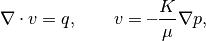
Compare the fine-scale and the multiscale solver for the single-phase pressure equation
![\nabla\cdot v = q, \qquad
v=\textbf{--}\frac{K}{\mu} \bigl[\nabla p+\rho g\nabla z\bigr],](_images/math/c264092627fac11273b12990e05ce27c1518c064.png)
This example is a direction continuation of “My First Flow-Solver: Gravity Column” and introduces the multiscale flow solver without going into specific details. More details can be found in the “Basic Multiscale Tutorial”.
mrstModule add coarsegrid mimetic msmfem incomp
Define the model
The domain [0,1]x[0,1]x[0,30] is discretized using a Cartesian grid with homogeneous isotropic permeability of 100 mD. The fluid has density 1000 kg/m^3 and viscosity 1 cP and the pressure is 100 bar at the top of the structure
nx = 2; ny = 2; nz = 30;
Nx = 1; Ny = 1; Nz =  6;
gravity reset on
G          = cartGrid([nx, ny, nz], [1, 1, 30]);
G          = computeGeometry(G);
rock.perm  = repmat(0.1*darcy(), [G.cells.num, 1]);
fluid      = initSingleFluid('mu' ,    1*centi*poise     , ...
                             'rho', 1014*kilogram/meter^3);

bc         = pside([], G, 'TOP', 100.*barsa);
Assemble and solve the fine-scale linear system
S   = computeMimeticIP(G, rock);
sol = incompMimetic(initResSol(G , 0.0), G, S, fluid, 'bc', bc);
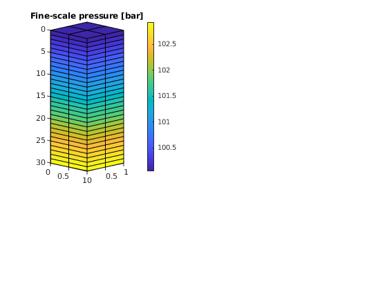
Plot the fine-scale solution
newplot;
subplot(3, 2, [1 3])
   plotCellData(G, convertTo(sol.pressure(1:G.cells.num), barsa), ...
                'EdgeColor', 'k');
   set(gca, 'ZDir', 'reverse'), title('Fine-scale pressure [bar]')
   view(45,5), cx = caxis; colorbar
Multiscale system
p  = partitionUI(G, [Nx, Ny, Nz]);
p  = processPartition  (G, p);
CG = generateCoarseGrid(G, p);

CS = generateCoarseSystem(G, rock, S, CG, ones([G.cells.num, 1]),'bc', bc);
xrMs = solveIncompFlowMS (initResSol(G, 0.0), G, CG, p, ...
                          S, CS, fluid, 'bc', bc);
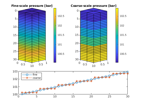
Plot the coarse-scale solution
As one clearly can see from the plot, the multiscale solution only captures the gravity effect on the coarse scale. To also capture fine-scale gravity effects, one can either add extra correction functions or insert the multiscale solution into the fine-scale equations and solve for a residual correction
subplot(3, 2, [2 4])
   plotCellData(G, convertTo(xrMs.pressure(1:G.cells.num), barsa), ...
                'EdgeColor', 'k');
   set(gca, 'ZDir', 'reverse'); title('Coarse-scale pressure [bar]')
   view(45,5); caxis(cx); colorbar

subplot(3, 2, [5 6]);
   plot(1:nz, convertTo(sol .pressure(1:nx*ny:nx*ny*nz), barsa()), '-o',...
        1:nz, convertTo(xrMs.pressure(1:nx*ny:nx*ny*nz), barsa()), '-*');
   legend('fine','coarse','Location','NorthWest');
Basic Multiscale Tutorial
Generated from simpleBCMS.m
The purpose of this example is to give an overview of how to set up and use the multiscale mimetic pressure solver in its hybrid formulation. To this end, we will compare the fine-grid and the multiscale solution of the single-phase pressure equation
for a Cartesian grid with lognormal, anisotropic permeability. This example is built upon the setup used in the “Basic Flow-Solver Tutorial”.
mrstModule add coarsegrid mimetic msmfem incomp
Define and visualize the model
We construct the Cartesian grid, set a lognormal anisotropic permeability with mean equal [1000 100 10] mD, and use the default single-phase fluid with unit viscosity
verbose = true;
nx = 10; ny = 10; nz = 4;
Nx =  5; Ny =  5; Nz = 2;

G         = cartGrid([nx, ny, nz],[100 100 40]*meter);
G         = computeGeometry(G);
K         = logNormLayers([nx, ny, nz], 1); K = 10 * K / mean(K(:));
rock.perm = bsxfun(@times, [10, 1, 0.1], convertFrom(K, milli*darcy()));
fluid     = initSingleFluid('mu' ,    1*centi*poise     , ...
                            'rho', 1014*kilogram/meter^3);

gravity off
Set boundary conditions: a flux of 1 m^3/day on the global left-hand side Dirichlet boundary conditions p = 0 on the global right-hand side of the grid, respectively.
bc = fluxside([], G, 'LEFT',  100*meter()^3/day());
bc = pside   (bc, G, 'RIGHT', 0);
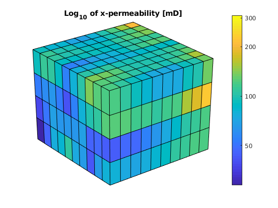
After the grid structure is generated, we plot the permeability and the geometry
newplot
plotCellData(G,log10(convertTo(rock.perm(:,1),milli*darcy))); shading faceted;
title('Log_{10} of x-permeability [mD]');
view(3), camproj perspective, axis tight off
cs = [50 100:100:1000];
h=colorbar; set(h,'YTick',log10(cs),'YTickLabel',cs');
Partition the grid
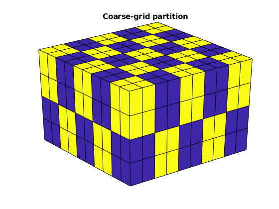
We partition the fine grid into a regular Nx-by-Ny-by-Nz coarse grid in index space so that each coarse block holds (nx/Nx)-by-(ny/Ny)-by-(nz/Nz) fine cells. The resulting vector p has one entry per fine-grid cell giving the index of the corresponding coarse block. After the grid is partitioned in index space, we postprocess it to make sure that all blocks consist of a connected set of fine cells. This step is superfluous for Cartesian grids, but is required for grids that are only logically Cartesian (e.g., corner-point and other mapped grids that may contain inactive or degenerate cells).
p  = partitionUI(G, [Nx, Ny, Nz]);
p  = processPartition(G, p);

% Plot the partition
newplot
plotCellData(G,mod(p,2)); shading faceted;
view(3); camproj perspective, axis tight off;
title('Coarse-grid partition');
Having obtain a partitioning in which each coarse block is a connected collection of cells from the fine grid, we build the coarse-grid structure, which is quite similar to that of the fine grid
CG = generateCoarseGrid(G, p, 'Verbose', verbose);
display(CG); disp(CG.cells); disp(CG.faces);
CG =

  struct with fields:

        cells: [1×1 struct]
        faces: [1×1 struct]
    partition: [400×1 double]
...
Build linear systems
First we compute the mimetic inner product and build the linear system for the fine-scale equations
S  = computeMimeticIP(G, rock, 'Verbose', verbose);
display(S);
Using inner product: 'ip_simple'.
Computing cell inner products ...             Elapsed time is 0.027574 seconds.
Assembling global inner product matrix ...    Elapsed time is 0.000524 seconds.

S =

  struct with fields:

...
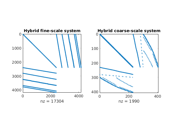
We generate the coarse-scale system by solving local flow problems,
one for each interface in the coarse grid. The basis functions for velocity and pressure are stored in two matrices. Unlike the fine-grid system, the B part of the hybrid system is not formed explicitly as a matrix block but constructed as a matrix product in our flow solver:
![A x = \left[\begin{array}{ccc}
\Psi^T B_f\Psi & C & D \\ C' & 0 & 0 \\ D' & 0 & 0
\end{array}\right]
\left[\begin{array}{c} v \\ \textbf{--}p \\ \lambda \end{array}\right]
= [\mbox{RHS}] = b,](_images/math/7100b7c334e46fe5df034a68667122c292b694c5.png)
where B_f is the fine-scale B-block and Psi contains the basis functions. In the structure, we store BPsi rather than Psi
CS = generateCoarseSystem(G, rock, S, CG, ones([G.cells.num, 1]), ...
                          'Verbose', verbose, 'bc', bc);
display(CS);
Computing flux and pressure basis functions... Elapsed time is 0.310659 seconds.

CS =

  struct with fields:

              basis: {195×1 cell}
             basisP: {195×1 cell}
...
The linear hybrid system for the coarse-scale equations has a similar structure as the corresponding fine-scale system, but with significantly fewer unknowns.
newplot;
subplot(1,2,1),
cellNo  = rldecode(1:G.cells.num, diff(G.cells.facePos), 2) .';
C       = sparse(1:numel(cellNo), cellNo, 1);
D       = sparse(1:numel(cellNo), double(G.cells.faces(:,1)), 1, ...
                 numel(cellNo), G.faces.num);

   spy([S.BI                  , C        , D        ; ...
        C', zeros(size(C,2), size(C,2) + size(D,2)); ...
        D', zeros(size(D,2), size(C,2) + size(D,2))]);
   title('Hybrid fine-scale system')

subplot(1,2,2),
   spy(msMatrixStructure(G, CG, 'bc', bc));
   title('Hybrid coarse-scale system');
Solve the global flow problems
xRef = incompMimetic    (initResSol(G, 0.0),  G, S, fluid, ...
                         'bc', bc, 'MatrixOutput',true);
xMs  = solveIncompFlowMS(initResSol(G, 0.0), G, CG, p, S, CS, fluid, ...
                         'bc', bc, 'MatrixOutput', true, 'Solver', 'hybrid');
Inspect the results
First we compare the Schur complement matrices
clf;
   subplot(1,2,1); spy(xRef.A); title('Schur complement matrix, fine scale');
   subplot(1,2,2); spy(xMs.A);  title('Schur complement matrix, coarse scale');
Then we compare the pressures and the flux intensities
clf
plot_var  = @(x) plotCellData(G, x);
plot_pres = @(x) plot_var(convertTo(x.pressure(1:G.cells.num), barsa()));
plot_flux = @(x) plot_var(accumarray(cellNo, ...
   abs(convertTo(faceFlux2cellFlux(G, x.flux), meter^3/day))));

subplot('Position',[0.02 0.52 0.46 0.42]),
   plot_pres(xRef); title('Pressure, fine [bar]')
   view(3), camproj perspective, axis tight equal, camlight headlight
   cax = caxis; colorbar

subplot('Position',[0.52 0.52 0.46 0.42]),
   plot_pres(xMs); title('Pressure, ms [bar]')
   view(3), camproj perspective, axis tight equal, camlight headlight
   caxis(cax); colorbar

subplot('Position',[0.02 0.02 0.46 0.42]),
   plot_flux(xRef); title('Flux intensity, fine')
   view(3), camproj perspective, axis tight equal, camlight headlight
   cax2 = caxis; colorbar

subplot('Position',[0.52 0.02 0.46 0.42]),
   plot_flux(xMs); title('Flux intensity, ms')
   view(3), camproj perspective, axis tight equal, camlight headlight
   caxis(cax2); colorbar
Multiscale Pressure Solver: Simple Corner-Point Grid with Linear Pressure Drop
Generated from simpleCornerPointExampleMS.m
Compare the fine-grid and the multiscale pressure solver by solving the single-phase pressure equation
for a simple corner-point grid model with isotropic, lognormal permeability. This example is built upon the flow-solver tutorial “A Simple Corner-Point Model”, but herein we generate a different version of the test grid that has a single fault.
try
   require coarsegrid mimetic msmfem incomp
catch
   mrstModule add coarsegrid mimetic msmfem incomp
end
Define and visualize the model
We construct a corner-point grid that with sloping pillars and wavy layers, construct a lognormal layered permeability field and use the default single-phase fluid with unit viscosity
nx = 20; ny = 20; nz = 8;
Nx =  5; Ny =  4; Nz = 2;
verbose = true;
grdecl  = simpleGrdecl([nx, ny, nz], 0.15);
G       = processGRDECL(grdecl); clear grdecl;
G       = computeGeometry(G);
Set fluid and rock properties
[rock.perm, L] = logNormLayers([nx, ny, nz], [100, 400, 50, 500]);
fluid          = initSingleFluid('mu' ,    1*centi*poise     , ...
                                 'rho', 1014*kilogram/meter^3);
rock.perm      = convertFrom(rock.perm, milli*darcy);  % mD -> m^2
Boundary conditions: pressure of one bar on the west-side boundary and zero on the east-side boundary.
westFaces = find(G.faces.centroids(:,1) == 0);
bc        = addBC([], westFaces, 'pressure',        ...
                  repmat(1*barsa(), [numel(westFaces), 1]));

xMax      = max(G.faces.centroids(:,1));
eastFaces = find(G.faces.centroids(:,1) == xMax);
bc        = addBC(bc, eastFaces, 'pressure',        ...
                  repmat(0, [numel(eastFaces), 1]));
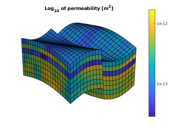
We visualize the model, performing a trick to manipulate the labels of the color bar to show the underlying values rather than the logarithm
clf
   plotCellData(G, log10(rock.perm(:))); shading faceted
   title('Log_{10} of permeability [m^2]')
   view(3), camproj perspective, axis tight off, camlight headlight
   h = colorbar; c = round(caxis); c = c(1) : c(2);
   set(h, 'YTick', c, 'YTickLabel', num2str(10.^c'));
Partition the grid
We partition the fine grid into coarse blocks, ensuring that the coarse blocks do not cross the layers in our model (given by the vector L).
p = partitionLayers(G, [Nx, Ny], L);
subplot('Position',[0.02 0.15 0.46 0.7]),
plotCellData(G, mod(p,9)); shading faceted;
outlineCoarseGrid(G,p,'LineWidth',3);
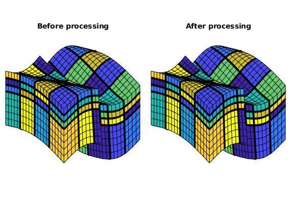
view(3), axis tight off, title('Before processing');
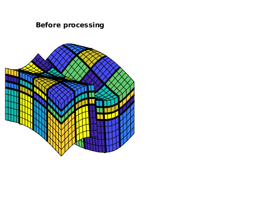
Here we can see that several blocks are disconnected over the fault. We therefore postprocess the grid to make sure that all blocks consist of a connected set of fine cells. Whereas this step is superfluous for Cartesian grids, the example shows that it is required for grids that are only logically Cartesian (e.g., corner-point and other mapped grids that may contain non-neighbouring connections and inactive or degenerate cells).
p = processPartition(G, p);
subplot('Position',[0.52 0.15 0.46 0.7]),
   plotCellData(G, mod(p,9)); shading faceted
   outlineCoarseGrid(G,p,'LineWidth',3);
   view(3), axis tight off, title('After processing');
Having obtained a reasonable partitioning, we build the coarse-grid structure.
CG = generateCoarseGrid(G, p, 'Verbose', verbose);
Assemble and solve system
Finally, we assemble the mimetic system in hybrid form and solve the corresponding linear equations.
S = computeMimeticIP(G, rock, 'Verbose', true);
xRef = incompMimetic(initResSol(G, 0), G, S, fluid, ...
                     'MatrixOutput', true, 'bc', bc);

mu  = fluid.properties(xRef);
kr  = fluid.relperm(ones([G.cells.num, 1]), xRef);
mob = kr ./ mu;

CS = generateCoarseSystem(G, rock, S, CG, mob, ...
                          'bc', bc, 'Verbose', verbose);
xMs = solveIncompFlowMS(initResSol(G, 0), G, CG, p, S, CS, fluid, ...
                        'bc', bc, 'Solver', S.type, 'MatrixOutput', true);
Using inner product: 'ip_simple'.
Computing cell inner products ...             Elapsed time is 0.241780 seconds.
Assembling global inner product matrix ...    Elapsed time is 0.001782 seconds.
Computing flux and pressure basis functions... Elapsed time is 0.893508 seconds.
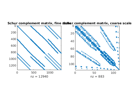
Plot Schur complement matrices
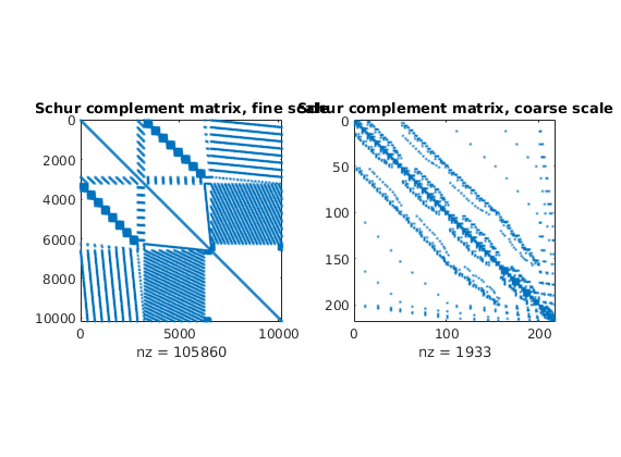
The Schur complement matrices are formed as part of the solution process and it can be instructive to see how this matrix differs on the fine and coarse scale
clf,
subplot(1,2,1), spy(xRef.A), title('Schur complement matrix, fine scale');
subplot(1,2,2), spy(xMs.A),  title('Schur complement matrix, coarse scale');
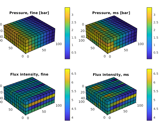
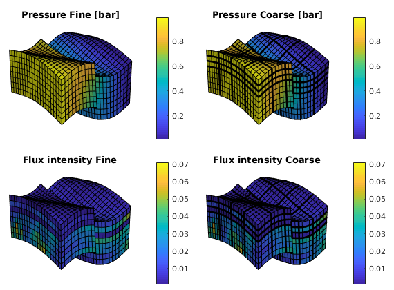
Plot results
We end the example by comparing pressures and fluxes computed on the fine and the coarse scale
clf
cellNo  = rldecode(1:G.cells.num, diff(G.cells.facePos), 2) .';
plot_var  = @(x) plotCellData(G, x);
plot_pres = @(x) plot_var(convertTo(x.pressure(1:G.cells.num), barsa()));
plot_flux = @(x) plot_var(accumarray(cellNo, ...
   abs(convertTo(faceFlux2cellFlux(G, x.flux), meter^3/day))));

subplot('Position',[0.02 0.52 0.46 0.42]),
   plot_pres(xRef); shading faceted, title('Pressure Fine [bar]')
   view(3), camproj perspective, axis tight off, camlight headlight
   cax = caxis; colorbar

subplot('Position',[0.52 0.52 0.46 0.42]),
   plot_pres(xMs);
   outlineCoarseGrid(G, p, 'FaceColor', 'none', 'LineWidth', 2);
   title('Pressure Coarse [bar]')
   view(3), camproj perspective, axis tight off, camlight headlight
   caxis(cax); colorbar

subplot('Position',[0.02 0.02 0.46 0.42]),
   plot_flux(xRef); shading faceted, title('Flux intensity Fine')
   view(3), camproj perspective, axis tight off, camlight headlight
   cax2 = caxis; colorbar

subplot('Position',[0.52 0.02 0.46 0.42]),
   plot_flux(xMs); title('Flux intensity Coarse')
   outlineCoarseGrid(G, p, 'FaceColor', 'none', 'LineWidth', 2);
   view(3), camproj perspective, axis tight off, camlight headlight
   caxis(cax2); colorbar
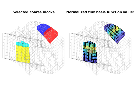
Plot a few selected flux basis functions
Finally, we display a graphical representation of a few flux basis functions. Relying on the fact that function ‘processPartition’ preserves the index of unsplit coarse blocks, we compute the index of the coarse block at original coarse logical position (5,2,1) and its Cartesian neighbour (5,3,1). Similarly, we compute the block index of the coarse block at original coarse position (2,3,3) and its Cartesian lower neighbour (2,3,4).
part_size = [Nx, Ny, numel(L) - 1];  % Cartesian size of original partition
b521 = sub2ind(part_size, 5, 2, 1);
b531 = sub2ind(part_size, 5, 3, 1);

b233 = sub2ind(part_size, 2, 3, 3);
b234 = sub2ind(part_size, 2, 3, 4);

disp('Block numbers:')
disp([b521, b531; b233, b234])
Block numbers:
    10    15
    52    72
The flux basis functions are stored in a packed data structure indexed by coarse faces. We therefore need to retrieve the face numbers of the coarse faces connecting each of the coarse block pairs defined above. This information is indirectly available in the coarse grid topology matrix, CG.faces.neigbors. As the block numbers may come in any order on a row in the topology matrix, we sort the individual rows to have a deterministic sort order.
faces = find(ismember(sort(CG.faces.neighbors      , 2), ...
                      sort([b521, b531; b233, b234], 2), 'rows')) %#ok
faces =

   165
   276
We now extract the individual basis functions values on ‘faces’. A further complication is that the actual values stored in the packed storage format is ‘B’ times the flux values, so we need to multiply by the inverse ‘B’ matrix, S.BI, in order to extract the flux values.
bf = S.BI * extractBF({ CS.basis{faces} }, size(G.cells.faces,1), CG);
Finally, compute plotting data (accumulated total flux in each cell) for each individual basis function, and normalize the data to have same colour limit for each basis function.
d = sparse(cellNo, 1 : size(G.cells.faces,1), 1) * abs(bf);
d = full(bsxfun(@rdivide, d, max(d)));
Extract the fine-scale cells in each of the four coarse blocks for plotting purposes.
blk_cells = @(b) find(p == b);
b521 = blk_cells(b521); b531 = blk_cells(b531);  % Connected by faces(1)
b233 = blk_cells(b233); b234 = blk_cells(b234);  % Connected by faces(2)

clf
   subplot('Position', [0.02, 0.15, 0.46, 0.7]),
   plotGrid(G, 'FaceColor', 'none',   'EdgeAlpha', 0.1);
   plotGrid(G, b521, 'FaceColor', 'r', 'EdgeAlpha', 0.1, 'FaceAlpha', 0.5);
   plotGrid(G, b531, 'FaceColor', 'b', 'EdgeAlpha', 0.1, 'FaceAlpha', 0.5);
   plotGrid(G, b233, 'FaceColor', 'c', 'EdgeAlpha', 0.1, 'FaceAlpha', 0.5);
   plotGrid(G, b234, 'FaceColor', 'y', 'EdgeAlpha', 0.1, 'FaceAlpha', 0.5);
   view(3), axis tight off, title('Selected coarse blocks')

   subplot('Position', [0.52, 0.15, 0.46, 0.7]),
   plotGrid(G, 'FaceColor', 'none',      'EdgeAlpha', 0.1);
   plotCellData(G, d(:,1), [b521; b531], 'FaceAlpha', 0.5);
   plotCellData(G, d(:,2), [b233; b234], 'FaceAlpha', 0.5);
   view(3), axis tight off, title('Normalized flux basis function values')
% simpleMSBCExample
% The example shows how to put Dirichlet boundary conditions on the system.
mrstModule add coarsegrid mimetic msmfem incomp


cellDims = [40, 40, 10];
verbose  = true;

gravity off;

G = cartGrid(cellDims, cellDims);
G = computeGeometry(G);

rock.perm = repmat(100*milli*darcy, [G.cells.num, 1]);
rock.poro = repmat(0.3            , [G.cells.num, 1]);
W = struct([]);
W = verticalWell(W, G, rock, 40, 40, 1:10, ...
                 'InnerProduct', 'ip_simple', ...
                 'Type', 'rate', 'Val', 1*meter^3/day, ...
                 'Radius', .1, 'Name', 'I');
W = addWell(W, G, rock, 1:40, 'Type','bhp', ...
            'InnerProduct', 'ip_simple', ...
            'Val', 0, 'Radius', .1, 'Dir', 'x', 'Name', 'P');

fluid = initSimpleFluid('mu' , [   1,  10]*centi*poise     , ...
                        'rho', [1000, 700]*kilogram/meter^3, ...
                        'n'  , [   2,   2]);
xrRef = initResSol(G, 0.0);

p  = partitionUI(G, [5, 5, 2]);
p  = processPartition  (G, p);
CG = generateCoarseGrid(G, p, 'Verbose', verbose);
S  = computeMimeticIP(G, rock, 'Verbose', verbose);
%
bc = pside([], G, 'LEFT', 0);
CS = generateCoarseSystem(G, rock, S, CG, ones([G.cells.num, 1]), ...
                          'Verbose', verbose, 'bc', bc);

W = generateCoarseWellSystem(G, S, CG, CS, ones([G.cells.num, 1]), rock, W);

xRef = initState(G, W, 0);
xMs  = initState(G, W, 0);

xRef = incompMimetic    (xRef, G, S, fluid, 'bc', bc, 'wells', W);
xMs  = solveIncompFlowMS(xMs, G, CG, p, S, CS, fluid, 'wells', W, ...
                         'bc', bc);
Using inner product: 'ip_simple'.
Computing cell inner products ...             Elapsed time is 1.075001 seconds.
Assembling global inner product matrix ...    Elapsed time is 0.009567 seconds.
Computing flux and pressure basis functions... Elapsed time is 1.162586 seconds.
Warning: Inconsistent Number of Phases.  Using 2 Phases (=min([3, 2, 2])).
plot output
Generated from simpleMSBCExample.m
f = figure;
cellNo = rldecode(1 : G.cells.num, diff(G.cells.facePos), 2) .';
plot_var = @(x) plotCellData(G, x, 'EdgeAlpha', 0.125);
plot_pres = @(x) plot_var(convertTo(x.pressure(1:G.cells.num), barsa));
plot_flux = @(x) plot_var(log10(accumarray(cellNo, ...
   abs(convertTo(faceFlux2cellFlux(G, x.flux), meter^3/day)))));
subplot(2,2,1)
   plot_pres(xRef); title('Pressure Fine [bar]')
   view(3), camproj perspective, axis tight equal, camlight headlight
   cax = caxis; colorbar

subplot(2,2,2)
   plot_pres(xMs); title('Pressure Coarse [bar]')
   view(3), camproj perspective, axis tight equal, camlight headlight
   caxis(cax);
   colorbar

subplot(2,2,3)
   plot_flux(xRef); title('Flux intensity Fine')
   view(3), camproj perspective, axis tight equal, camlight headlight
   cax2 = caxis; colorbar

subplot(2,2,4)
   plot_flux(xMs); title('Flux intensity Coarse')
   view(3), camproj perspective, axis tight equal, camlight headlight
   caxis(cax2); colorbar
Multiscale Pressure Solver: Flow Driven by Horizontal and Vertical Well
Generated from simpleMSExample.m
Compare the fine-grid and the multiscale pressure solver by solving the single-phase pressure equation
for a Cartesian grid with isotropic, homogeneous permeability
mrstModule add coarsegrid mimetic msmfem incomp
Define and visualize the model
We construct the Cartesian grid, set the permeability to 100 mD, and use the default single-phase fluid with unit viscosity
cellDims  = [40, 40, 10];
verbose   = mrstVerbose;
G         = cartGrid(cellDims, cellDims);
G         = computeGeometry(G);
rock.perm = repmat(100*milli*darcy, [G.cells.num, 1]);
fluid     = initSimpleFluid('mu' , [   1,  10]*centi*poise     , ...
                            'rho', [1000, 700]*kilogram/meter^3, ...
                            'n'  , [   2,   2]);

% Set two wells, one vertical and one horizontal
W = struct([]);
W = verticalWell(W, G, rock, 40, 40, 1:10, ...
                 'InnerProduct', 'ip_simple', ...
                 'Type', 'rate', 'Val', 1*meter^3/day, ...
                 'Radius', .1, 'Name', 'I');
W = addWell(W, G, rock, 1:40, 'Type','bhp', ...
            'InnerProduct', 'ip_simple', ...
            'Val', 0, 'Radius', .1, 'Dir', 'x', 'Name', 'P');

% Visualize the model
figure;
plotGrid(G, 'FaceColor', 'none', 'EdgeColor', [0.65, 0.65, 0.65]);
plotWell(G, W, 'radius', 0.1, 'color', 'r');
view(3); axis equal tight off

Set up solution structures
Here we need four solution structures, two for each simulator to hold the solutions on the grid and in the wells, respectively.
xRef = initState(G, W, 0);
xMs  = initState(G, W, 0);
Partition the grid
We partition the fine grid into a regular 5-by-5-by-2 coarse grid in index space so that each coarse block holds 8-by-8-by-5 fine cells. The resulting vector p has one entry per fine-grid cell giving the index of the corresponding coarse block. After the grid is partitioned in index space, we postprocess it to make sure that all blocks consist of a connected set of fine cells. This step is superfluous for Cartesian grids, but is required for grids that are only logically Cartesian (e.g., corner-point and other mapped grids that may contain inactive or degenerate cells).
p  = partitionUI(G, [5, 5, 2]);
p  = processPartition(G, p);

figure;
plotCellData(G,mod(p,2)); view(3); axis equal tight off

CG = generateCoarseGrid(G, p, 'Verbose', verbose);

S  = computeMimeticIP(G, rock, 'Verbose', verbose);
CS = generateCoarseSystem (G, rock, S, CG, ones([G.cells.num, 1]), ...
                           'Verbose', verbose);

W = generateCoarseWellSystem(G, S, CG, CS, ones([G.cells.num, 1]), rock, W);

xRef = incompMimetic    (xRef, G, S, fluid, 'wells', W, 'Solver', 'hybrid');
xMs  = solveIncompFlowMS(xMs, G, CG, p, S, CS, fluid, 'wells', W, ...
                         'Solver', 'hybrid');

dp = @(x) num2str(convertTo(x(1).pressure, barsa));
disp(['DeltaP - Fine: ', dp(xRef.wellSol)]);
disp(['DeltaP - Ms:   ', dp(xMs .wellSol)]);
DeltaP - Fine: 3.7478
DeltaP - Ms:   3.7875

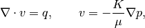
plot output
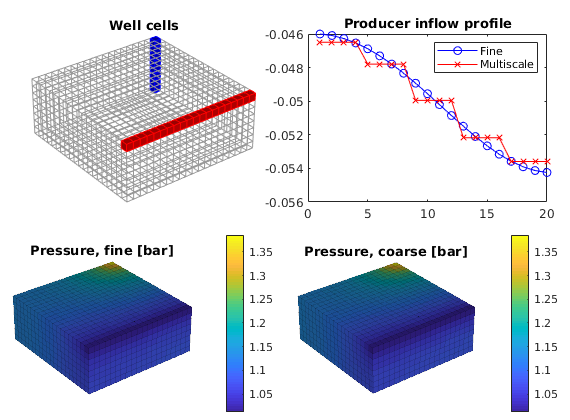
f = figure;
subplot(2,2,1)
   plotGrid(G, 'FaceColor', 'none', 'EdgeColor', [.6, .6, .6]);
   plotGrid(G, W(1).cells, 'FaceColor', 'b', 'EdgeColor', 'b');
   plotGrid(G, W(2).cells, 'FaceColor', 'r', 'EdgeColor', 'r');
   title('Well cells')
   view(3); camproj perspective; axis tight; axis equal; camlight headlight;

subplot(2,2,2)
   plot(convertTo(xRef.wellSol(2).flux, meter^3/day), 'b'); hold on
   plot(convertTo(xMs.wellSol (2).flux, meter^3/day), 'r');
   legend('Fine','Multiscale')
   title('Producer inflow profile')

subplot(2,2,3)
   plotCellData(G, convertTo(xRef.pressure, barsa), 'EdgeAlpha', 0.125);
   title('Pressure Fine')
   view(3), camproj perspective, axis tight equal, camlight headlight
   cax = caxis; colorbar

subplot(2,2,4)
   plotCellData(G, convertTo(xMs.pressure, barsa), 'EdgeAlpha', 0.125);
   title('Pressure Coarse')
   view(3), camproj perspective, axis tight equal, camlight headlight
   caxis(cax); colorbar
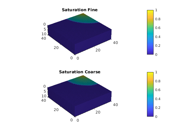
function simpleMSSourceExample(varargin)
simpleMSSourceExample -- Demonstrate handling of explicit sources in
%                          multiscale pressure solvers.
%
% SYNOPSIS:
%   simpleMSSourceExample()
%
% PARAMETERS:
%   None.
%
% RETURNS:
%   Nothing
Using inner product: 'ip_simple'.
Computing cell inner products ...             Elapsed time is 0.001910 seconds.
Assembling global inner product matrix ...    Elapsed time is 0.000210 seconds.
Alternative 1:
Generated from simpleMSSourceExample.m
Call addSource before calling generateCoarseSystem: The fine-scale sources will then be put correctly into the coarse system in ‘generateCoarseSystem’ and basis functions are also generated correctly.
src = addSource([], [1, G.cells.num], ...
                   [-1, 1] ./ day(), 'sat', [1, 0, 0; 1, 0, 0]);

   CS = generateCoarseSystem (G, rock, S, CG, ones([G.cells.num, 1]), ...
                              'Verbose', verbose, 'src', src);

   xRef = incompMimetic    (xRef, G, S, fluid, 'src', src);
   xMs  = solveIncompFlowMS(xMs , G, CG, p, S, CS, fluid, 'src', src);

   % Plot result:
   plot_res(figure, G, xRef, xMs);
%{
   %% Alternative 2:
   % Add source/sink by calling putSourceMS can after generateCoarseSystem
   % is called.
   % Function 'putSourceMS' will update S, CS and CS.basis. W must be re-assembeled.
   %
   src = addSource([], [100; 200], [-1; 1], 'sat', [1, 0, 0; 1, 0, 0]);
   [S, CS] = putSourceMS(G, S, CG, CS, rock, src);

   xrRef = incompMimetic    (xrRef, [], G, S, fluid, ...
                             'src', src);
   xrMs  = solveIncompFlowMS(initResSol(G, 0.0), [], ...
                             G, CG, p, S, CS, fluid, 'src', src)

   % Plot result:
   plot_res(figure, G, S, xrRef, xrMs);

   %% Remove source/sink
   [S, CS] = rmSourceMS(G, S, CG, CS, rock, [100 200]);
   %{

   xrRef = incompMimetic    (xrRef, [], G, S, fluid, ...
                             'src', src);
   xrMs  = solveIncompFlowMS(initResSol(G, 0.0), [], ...
                             G, CG, p, S, CS, fluid, 'src', src);
   %}

   % Plot result:
   plot_res(figure, G, S, xrRef, xrMs);
   %}
Computing flux and pressure basis functions... Elapsed time is 0.187178 seconds.
end

%--------------------------------------------------------------------------
% Helpers follow.
%--------------------------------------------------------------------------

function plot_res(f, g, xRef, xMs)
   cellno = rldecode(1 : g.cells.num, diff(g.cells.facePos), 2) .';
   plt  = @(v) plotCellData(g, v);
   pres = @(x) plt(convertTo(x.pressure(1:g.cells.num), barsa()));
   flux = @(x) plt(convertTo(sqrt(accumarray(cellno, ...
                                             faceFlux2cellFlux(g, x.flux).^ 2)), ...
                             meter^3 / day));

   set(0, 'CurrentFigure', f)

   subplot(2,2,1)
      pres(xRef); set_view(), title('Pressure Fine')
      cax = caxis; colorbar

   subplot(2,2,2)
      pres(xMs); set_view(), title('Pressure Coarse')
      caxis(cax), colorbar

   subplot(2,2,3)
      flux(xRef); set_view(), title('Flux intensity Fine')
      cax2 = caxis; colorbar

   subplot(2,2,4)
      flux(xMs); set_view(), title('Flux intensity Coarse')
      caxis(cax2), colorbar
end

%--------------------------------------------------------------------------

function set_view()
   view(3), camproj perspective, axis tight equal, camlight headlight
end
Multiscale Pressure Solver with Overlap:
Generated from simpleOverlap.m
Use overlap in multiscale basis function to improve accuracy of the simulation. We compare the fine-grid pressure solver and multiscale pressure solvers with and without overlap by solving the single-phase pressure equation
for a Cartesian grid with anisotropic, homogeneous permeability. Overlap means that we extend the support of the multiscale basis functions, that is, we include more fine cells when computing the basis function. The use of overlap is particularly attractive in cases of highly heterogeneous reservoirs and wells that are placed near the corner of a coarse well-block. In the following, let the dashed lines be the coarse grid, the dotted lines represent the overlap, and let ‘*’ represent a well.
mrstModule add coarsegrid mimetic msmfem incomp
Define and visualize the model
nx = 40; ny = 40; nz = 2;
cellDims = [nx, ny, nz];
G = cartGrid(cellDims);
G = computeGeometry(G);
diag_k = [500, 500, 50] .* (1e-3*darcy());
rock.perm = repmat(diag_k, [G.cells.num, 1]);
fluid = initSingleFluid('mu' , 1*centi*poise , ...
'rho', 1000*kilogram/meter^3);
% Set two vertical wells.
injCells = [ 8, 8];
prodCells = [33, 33];
W = struct([]);
W = verticalWell(W, G, rock, injCells(1), injCells(2), 1:2, ...
'InnerProduct', 'ip_simple', ...
'Type', 'rate', 'Val', 1*meter^3/day, ...
'Radius', 0.1);
W = verticalWell(W, G, rock, prodCells(1), prodCells(2), 1:2, ...
'InnerProduct', 'ip_simple', ...
'Type', 'bhp', 'Val', 0, 'Radius', 0.1);
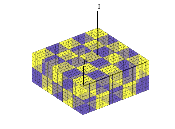
% Visualize the model.
clf
plotGrid(G, 'FaceColor', 'none', 'EdgeColor', [0.65, 0.65, 0.65]);
plotWell(G, W, 'radius', 0.1, 'color', 'r');
view(3), axis equal tight off
Partition the grid and assemble linear systems
part  = partitionCartGrid(cellDims, [5, 5, 1]);
CG    = generateCoarseGrid(G, part, 'Verbose', true);

gravity off
S  = computeMimeticIP(G, rock, 'Verbose', true);

% Note: Only use overlap around wells, not in reservoir basisfunctions
CS = generateCoarseSystem (G, rock, S, CG, ones([G.cells.num,1]), ...
                           'Verbose', true, 'Overlap', 0);
Using inner product: 'ip_simple'.
Computing cell inner products ...             Elapsed time is 0.255279 seconds.
Assembling global inner product matrix ...    Elapsed time is 0.002182 seconds.
Computing flux and pressure basis functions... Elapsed time is 0.295473 seconds.
Generate coarse well system with overlap around the well
For overlap in the well basis we has two different choices: ‘OverlapWell’ and ‘OverlapBlock’. The first includes cells around the well and the latter cells around the well-block (the coarse block containing the well). We apply overlap around the well for ‘W1’ and use no overlap for ‘W’ as a reference.
W1 = W;

% Calculate total mobility (needed by generateCoarse*System).
state = initResSol(G, 0, 1);
mu    = fluid.properties(state);
s     = fluid.saturation(state);
kr    = fluid.relperm(s, state);

totmob = sum(bsxfun(@rdivide, kr, mu), 2);    clear mu s kr state

% First no overlap
W  = generateCoarseWellSystem(G, S, CG, CS, totmob, rock, W, ...
                              'OverlapWell',  0, 'OverlapBlock', 0);
% Then overlap around well
W1 = generateCoarseWellSystem(G, S, CG, CS, totmob, rock, W1, ...
                              'OverlapWell', 10, 'OverlapBlock', 0);
Solve the global flow problems
% Fine scale reference solution:
xRef = initState(G, W, 0);
xRef = incompMimetic(xRef, G, S, fluid, 'wells', W);

% Coarse scale - no overlap:
xMs   = initState(G, W, 0);
xMs   = solveIncompFlowMS(xMs, G, CG, part, S, CS, fluid, ...
                          'wells', W, 'Solver', 'mixed');

% Coarse scale - overlap:
xMs1  = initState(G, W, 0);
xMs1  = solveIncompFlowMS(xMs1, G, CG, part, S, CS, fluid, ...
                          'wells', W1, 'Solver', 'mixed');

% Report pressure drop between wells.
dp = @(x) num2str(convertTo(x.wellSol(1).pressure, barsa()));
disp(['DeltaP - Fine:          ', dp(xRef)])
disp(['DeltaP - Ms no overlap: ', dp(xMs )])
disp(['DeltaP - Ms overlap:    ', dp(xMs1)])
Warning: Inconsistent Number of Phases.  Using 1 Phase (=min([3, 1, 1])).
DeltaP - Fine:          0.28562
DeltaP - Ms no overlap: 0.39031
DeltaP - Ms overlap:    0.28944
Plot solution
cellNo    = rldecode(1 : G.cells.num, diff(G.cells.facePos), 2) .';
diverg    = @(v) accumarray(cellNo, abs(convertTo(v, meter^3/day)));
plot_flux = @(v) plotCellData(G, diverg(v), 'EdgeAlpha', 0.125);
well_bas  = @(w) S.BI * sparse(w.CS.basis{1}{1}, 1, w.CS.basis{1}{3}, ...
                               size(G.cells.faces,1), 1);
figure;
subplot(2,3,1)
   plot_flux(faceFlux2cellFlux(G, xRef.flux));
   title('Flux - fine scale'); cx = caxis;

subplot(2,3,2)
   plot_flux(faceFlux2cellFlux(G, xMs.flux ));
   title('Flux - no overlap'); caxis(cx)

subplot(2,3,3)
   plot_flux(faceFlux2cellFlux(G, xMs1.flux));
   title('Flux - overlap')   ; caxis(cx)

subplot(2,3,5)
   plot_flux(full(well_bas(W(1))));
   axis([0, 20, 0, 20]);  cx = caxis;
   title('Well basis - no overlap')

subplot(2,3,6)
   plot_flux(full(well_bas(W1(1))));
   axis([0, 20, 0, 20]); caxis(cx);
   title('Well basis - overlap')

Multiscale: Sources and Boundary Conditions
Generated from simpleSRCandBCMS.m
Compare the fine-grid and the multiscale pressure solver by solving the single-phase pressure equation
for a Cartesian grid with lognormal, layered, isotropic permeability. This example is built upon the “Basic Multiscale Tutorial” and the flow-solver tutorial “How to Specify Sources and Boundary Conditions”.
mrstModule add coarsegrid mimetic msmfem incomp
Define and visualize the model
We construct the Cartesian grid, set a lognormal, layered, isotropic permeability with given mean, and use the default single-phase fluid with unit viscosity
nx = 20; ny = 20; nz = 20;
Nx = 5; Ny = 5;
G = cartGrid([nx ny nz]);
G = computeGeometry(G);
[K, L] = logNormLayers([nx, ny, nz], 100*rand([10, 1]));
rock.perm = convertFrom(K, milli*darcy);
fluid = initSingleFluid('mu' , 1*centi*poise , ...
'rho', 1014*kilogram/meter^3);
gravity reset on
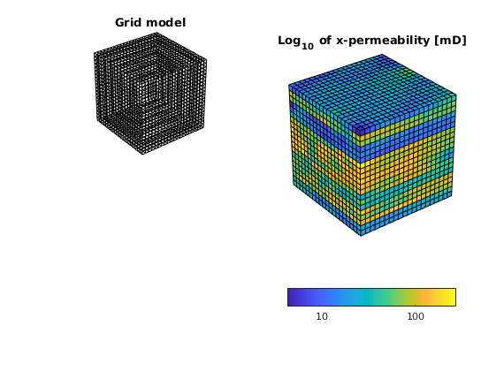
% To check that the model is correct, we plot it
subplot(2,2,1)
plotGrid(G,'FaceColor', 'none');
title('Grid model')
view(3), camproj perspective, axis tight equal off
subplot(2,2,[2 4])
plotCellData(G,log10(rock.perm(:,1)) ); shading faceted;
title('Log_{10} of x-permeability [mD]');
view(3), camproj perspective, axis tight equal off
h = colorbar('horiz'); dCorr = log10(darcy() / 1000);
cs = round(caxis - dCorr); cs = cs(1) : cs(2);
set(h, 'XTick', cs+dCorr, 'XTickLabel', num2str(10.^cs'));
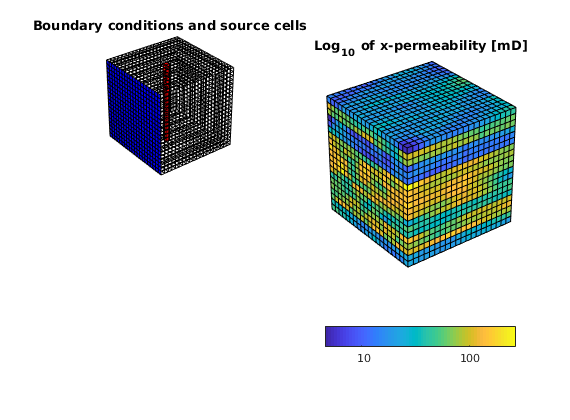
Model vertical well as a column of cell sources, each with rate equal 1 m^3/day.
c   = (nx/2*ny+nx/2 : nx*ny : nx*ny*nz) .';
src = addSource([], c, ones(size(c)) ./ day());
subplot(2,2,1); plotGrid(G, c, 'FaceColor', 'r');
title('Source cells');

Set boundary conditions: a Dirichlet boundary condition of p=10 bar at the global left-hand side of the model
bc = pside([], G, 'LEFT', 10*barsa());
subplot(2,2,1); plotFaces(G, bc.face, 'b');
title('Boundary conditions and source cells');
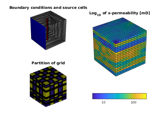
Partition the grid
We partition the fine grid into coarse blocks, ensuring that the coarse blocks do not cross the layers in our model (given by the vector L).
p = partitionLayers(G, [Nx, Ny], L);
p = processPartition(G, p);

subplot(2,2,3);
   plotCellData(G,mod(p,2)); shading faceted
   outlineCoarseGrid(G,p,'LineWidth',3);
   view(3); axis equal tight off
   title('Partition of grid');
Construct linear systems
We build the grid structure for the coarse grid and construct the fine and the coarse system
CG = generateCoarseGrid(G, p);
S  = computeMimeticIP(G, rock);
CS = generateCoarseSystem(G, rock, S, CG, ones([G.cells.num, 1]), ...
                          'bc', bc, 'src', src);
Solve the global flow problems
xRef = incompMimetic    (initResSol(G, 0.0), G, S, fluid, ...
                         'src', src, 'bc', bc);
xMs  = solveIncompFlowMS(initResSol(G, 0.0), G, CG, p, S, CS, fluid,  ...
                         'src', src, 'bc', bc);
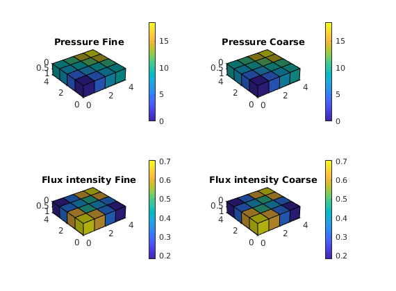
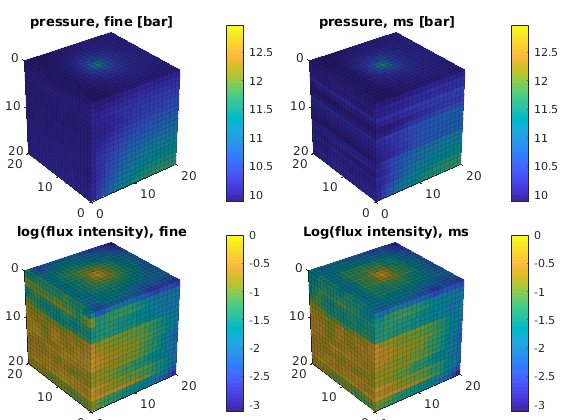
Plot solution
clf,
cellNo  = rldecode(1:G.cells.num, diff(G.cells.facePos), 2) .';
plot_var  = @(x) plotCellData(G, x, 'EdgeAlpha', 0.125);
plot_pres = @(x) plot_var(convertTo(x.pressure(1:G.cells.num), barsa()));
plot_flux = @(x) plot_var(log10(accumarray(cellNo, ...
   abs(convertTo(faceFlux2cellFlux(G, x.flux), meter^3/day)))));

subplot('Position',[0.02 0.52 0.46 0.42]),
   plot_pres(xRef); title('pressure, fine [bar]')
   view(3), camproj perspective, axis tight equal, camlight headlight
   cax = caxis; colorbar

subplot('Position',[0.52 0.52 0.46 0.42]),
   plot_pres(xMs); title('pressure, ms [bar]')
   view(3), camproj perspective, axis tight equal, camlight headlight
   caxis(cax); colorbar

subplot('Position',[0.02 0.02 0.46 0.42]),
   plot_flux(xRef); title('log(flux intensity), fine')
   view(3), camproj perspective, axis tight equal, camlight headlight
   cax2 = caxis; colorbar

subplot('Position',[0.52 0.02 0.46 0.42]),
   plot_flux(xMs); title('Log(flux intensity), ms')
   view(3), camproj perspective, axis tight equal, camlight headlight
   caxis(cax2); colorbar
Multiscale Pressure Solver: Flow Driven by Horizontal and Vertical Well
Generated from simpleWellExampleMS.m
Compare the fine-grid and the multiscale pressure solver by solving the single-phase pressure equation
for a Cartesian grid with isotropic, homogeneous permeability. This example is built upon the flow-solver tutorial “Using Peacemann well models”.
mrstModule add coarsegrid mimetic msmfem incomp
Define the model and set data
We construct the Cartesian grid, set the permeability to 100 mD, and use the default single-phase fluid with density 1000 kg/m^3 and viscosity 1 cP.
nx = 20; ny = 20; nz = 8;
Nx =  5; Ny =  5; Nz = 2;
verbose   = false;
G         = cartGrid([nx ny nz]);
G         = computeGeometry(G);
rock.perm = repmat(100*milli*darcy, [G.cells.num, 1]);
fluid     = initSingleFluid('mu' ,    1*centi*poise     , ...
                            'rho', 1014*kilogram/meter^3);
Set two wells, one vertical and one horizontal. Note that a vertical well can be constructed by both addWell and verticalWell, so the appropriate choice depends on whether you know the well cells or the I, J, K position of the well.
W = verticalWell([], G, rock, nx, ny, 1:nz,            ...
                 'InnerProduct', 'ip_simple',          ...
                'Type', 'rate', 'Val', 1*meter^3/day, ...
                'Radius', .1, 'Name', 'I', 'Comp_i', 1);
W = addWell(W, G, rock, 1:nx, 'Type','bhp', ...
            'InnerProduct', 'ip_simple', ...
            'Val', 1*barsa, 'Radius', .1, 'Dir', 'x', ...
            'Name', 'P', 'Comp_i', 0);
Set up solution structures
Here we need four solution structures, two for each simulator to hold the solutions on the grid and in the wells, respectively.
xRef = initState(G, W, 0, 1);
xMs  = xRef;
Partition the grid
We partition the fine grid into a regular Nx-by-Ny-by-Nz coarse grid in index space so that each coarse block holds (nx/Nx)-by-(ny/Ny)-by-(nz/Nz) fine cells. The resulting vector p has one entry per fine-grid cell giving the index of the corresponding coarse block. After the grid is partitioned in index space, we postprocess it to make sure that all blocks consist of a connected set of fine cells. This step is superfluous for Cartesian grids, but is required for grids that are only logically Cartesian (e.g., corner-point and other mapped grids that may contain inactive or degenerate cells).
p = partitionUI(G, [Nx, Ny, Nz]);
p = processPartition(G, p);

% Generate the coarse-grid structure
CG = generateCoarseGrid(G, p, 'Verbose', verbose);
Plot the partition and the well placement
clf
plotCellData(G, mod(p,2),'EdgeColor','k','FaceAlpha',0.5,'EdgeAlpha', 0.5);
plotWell(G, W, 'radius', 0.1, 'color', 'k');
view(3), axis equal tight off
Assemble linear systems
First we compute the inner product to be used in the fine-scale and coarse-scale linear systems. Then we generate the coarse-scale system
gravity off
S  = computeMimeticIP(G, rock, 'Verbose', verbose);

mu  = fluid.properties(xMs);
kr  = fluid.relperm(ones([G.cells.num, 1]), xMs);
mob = kr ./ mu;
CS  = generateCoarseSystem(G, rock, S, CG, mob, 'Verbose', verbose);
Then, we assemble the well systems for the fine and the coarse scale.
W = generateCoarseWellSystem(G, S, CG, CS, mob, rock, W);
disp('W(1):'); display(W(1));
disp('W(2):'); display(W(2));
W(1):
        cells: [8×1 double]
         type: 'rate'
          val: 1.1574e-05
            r: [8×1 double]
          dir: [8×1 char]
           rR: [8×1 double]
           WI: [8×1 double]
...
Solve the global flow problems
xRef = incompMimetic    (xRef, G, S, fluid, 'wells', W, ...
                         'Solver', S.type, 'MatrixOutput', true);
xMs  = solveIncompFlowMS(xMs , G, CG, p, S, CS, fluid, 'wells', W, ...
                         'Solver', S.type, 'MatrixOutput', true);

% Report pressure in wells.
dp = @(x) num2str(convertTo(x.wellSol(1).pressure, barsa));
disp(['DeltaP, Fine: ', dp(xRef)])
disp(['DeltaP, Ms:   ', dp(xMs )])
DeltaP, Fine: 1.4186
DeltaP, Ms:   1.423
Plot Schur complement matrices
clf
   subplot(1,2,1); spy(xRef.A); title('Schur complement matrix, fine scale');
   subplot(1,2,2); spy(xMs.A);  title('Schur complement matrix, coarse scale');
Plot solution
clf
subplot('Position', [0.02 0.52 0.46 0.42]),
plotGrid(G, 'FaceColor', 'none', 'EdgeColor', [.6, .6, .6]);
plotGrid(G, W(1).cells, 'FaceColor', 'b', 'EdgeColor', 'b');
plotGrid(G, W(2).cells, 'FaceColor', 'r', 'EdgeColor', 'r');
title('Well cells')
view(3), camproj perspective, axis tight equal off, camlight headlight
subplot('Position', [0.54 0.52 0.42 0.40]),
plot(convertTo(xRef.wellSol(2).flux, meter^3/day), '-ob'); hold on
plot(convertTo(xMs .wellSol(2).flux, meter^3/day), '-xr');
legend('Fine', 'Multiscale')
title('Producer inflow profile')
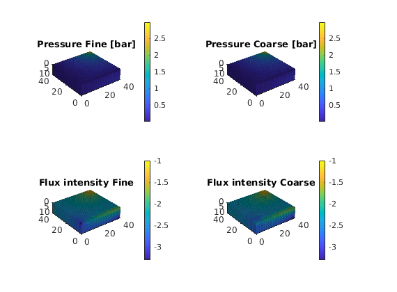
subplot('Position', [0.02 0.02 0.46 0.42]),
plotCellData(G, convertTo(xRef.pressure, barsa), 'EdgeAlpha', 0.125)
title('Pressure, fine [bar]')
view(3), camproj perspective, axis tight equal off, camlight headlight
cax = caxis; colorbar
subplot('Position', [0.52 0.02 0.46 0.42]),
plotCellData(G, convertTo(xMs.pressure, barsa), 'EdgeAlpha', 0.125);
title('Pressure, coarse [bar]')
view(3), camproj perspective, axis tight equal off, camlight headlight
caxis(cax); colorbar
Multiscale Pressure Solver with Overlap:
Generated from simpleWellOverlap.m
Use overlap in multiscale basis function to improve accuracy of the simulation. We compare the fine-grid pressure solver and multiscale pressure solvers with and without overlap by solving the single-phase pressure equation
for a Cartesian grid with anisotropic, homogeneous permeability. This example shows the use of overlap around the well.
mrstModule add coarsegrid mimetic msmfem incomp
What is overlap?
Overlap means that we extend the support of the multiscale basis functions, that is, we include more fine cells when computing the basis function. Using overlapping domains enables capturing more complex flow patterns, particularly for very coarse grids, at the expense of increased coupling in the resulting systems of linear equations. The use of overlap is particularly attractive in cases of highly heterogeneous reservoirs of cases where wells are placed near the corner of a coarse well-block. In the following, we describe the different types of overlap implemented in the Matlab Reservoir Simulation Toolbox. Let the thick lines be the coarse grid, the thin lines represent the fine grid, the shaded region the overlap (of fine cells), and the red circle be the well. Overlap in the reservoir basis function for a coarse face ij means that we include fine cells around the the neighboring coarse blocks when we compute the basis for face ij:
The flow near a well is described by a multiscale well basis. This basis normally only has support in the coarse well-block. If the well lies close to the corner of the well-block, this will be a poor description of the flow near the well because it will not describe the flow over the corner. In such cases we can use overlap around the well (‘overlapWell’), here shown in different colors with increasing number of overlap:
In some cases (e.g in case of highly hetereogeneous permeability) it might be necessary to use overlap around the entire well block (‘OverlapBlock’):
Define and visualize the model
We set up a simple 40-by-40-by-2 cartesian grid model with anisotropic, homogeneous permeability and assume that the reservoir is filled with a single fluid (with default values).
G         = cartGrid([40, 40, 2]);
G         = computeGeometry(G);
diag_k    = [500, 500, 50] .* milli*darcy;
rock.perm = repmat(diag_k, [G.cells.num, 1]);
fluid     = initSingleFluid('mu' ,    1*centi*poise     , ...
                            'rho', 1014*kilogram/meter^3);

gravity off

% Set two vertical wells.
W = verticalWell([], G, rock,  8,  8, 1:G.cartDims(3), ...
                 'InnerProduct', 'ip_simple', ...
                 'Type', 'rate', 'Val', 1*meter^3/day, ...
                 'Radius', 0.1, 'Comp_i', 1);
W = verticalWell(W , G, rock, 33, 33, 1:G.cartDims(3), ...
                 'InnerProduct', 'ip_simple', ...
                 'Type', 'bhp', 'Val', 0, 'Radius', 0.1, 'Comp_i', 0);
Partition the grid and compute mimetic innerproduct
We partition the fine grid uniformly into 5-by-5-by-1 blocks using no overlap in the basis reservoir basis functions.
part = partitionCartGrid(G.cartDims, [5, 5, 1]);
CG   = generateCoarseGrid(G, part);
S    = computeMimeticIP(G, rock);

% Note: Only use overlap around wells, not in reservoir basisfunctions
mu  = fluid.properties(initResSol(G, 0.0));
kr  = fluid.relperm(ones([G.cells.num, 1]), initResSol(G, 0.0));
mob = kr ./ mu;
CS  = generateCoarseSystem(G, rock, S, CG, mob, 'Overlap', 0);

clf,
   plotCellData(G, mod(part,2), 'EdgeColor', 'k');
   outlineCoarseGrid(G, part, 'LineWidth', 3);
   plotWell(G, W, 'radius', 0.1, 'height', 2);
   view(3), axis tight off
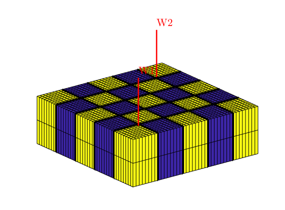
Generate coarse well system with overlap around the well
As can be seen from the plot of the model, the wells are near a corner of their supporting coarse blocks, which may lead to highly inaccurate results (as we will see shortly). To impreove the accuracy, we can introduce onverlap in the well basis functions. As pointed out above, we have two different choices: ‘OverlapWell’ and ‘OverlapBlock’. The first includes cells around the well and the latter includes cells around the well-block (the coarse block containing the well). We apply overlap around the well for ‘W1’ and use no overlap for ‘W’ as a reference.
W1 = W;

% First no overlap
W  = generateCoarseWellSystem(G, S, CG, CS, mob, rock, W, ...
                              'OverlapWell',  0, 'OverlapBlock', 0);
% Then overlap around well
W1 = generateCoarseWellSystem(G, S, CG, CS, mob, rock, W1, ...
                              'OverlapWell', 10, 'OverlapBlock', 0);
Solve the global flow problems
% Fine scale reference solution:
ref = initState(G, W, 0, 1);
ref = incompMimetic(ref, G, S, fluid, 'wells', W);

% Coarse scale - no overlap:
s = initState(G, W, 0, 1);
s = solveIncompFlowMS(s,  G, CG, part, S, CS, fluid, ...
                      'wells', W, 'Solver', 'mixed');

% Coarse scale - overlap:
s1 = initState(G, W, 0, 1);
s1 = solveIncompFlowMS(s1, G, CG, part, S, CS, fluid, ...
                       'wells', W1, 'Solver', 'mixed');

% Report pressure drop between wells.
dp = @(x) num2str(convertTo(x.wellSol(1).pressure, barsa()));
disp(['DeltaP - Fine:          ', dp(ref)])
disp(['DeltaP - Ms no overlap: ', dp(s  )])
disp(['DeltaP - Ms overlap:    ', dp(s1 )])
DeltaP - Fine:          0.28562
DeltaP - Ms no overlap: 0.39031
DeltaP - Ms overlap:    0.28944
Plot solution
cellNo    = rldecode(1 : G.cells.num, diff(G.cells.facePos), 2) .';
diverg    = @(v) accumarray(cellNo, abs(convertTo(v, meter^3/day)));
plot_flux = @(x) plotCellData(G, diverg(x), 'EdgeAlpha', 0.125);
well_bas  = @(w) S.BI * sparse(w.CS.basis{1}{1}, 1, w.CS.basis{1}{3}, ...
                               size(G.cells.faces,1), 1);

subplot(2,3,1)
   plot_flux(ref.flux(G.cells.faces(:,1)));
   title('Flux - fine scale'); cx = caxis;

subplot(2,3,2)
   plot_flux(s.flux(G.cells.faces(:,1)))  ;
   title('Flux - no overlap'); caxis(cx)

subplot(2,3,3)
   plot_flux(s1.flux(G.cells.faces(:,1))) ;
   title('Flux - overlap')   ; caxis(cx)

subplot(2,3,5)
   plot_flux(full(well_bas(W(1))));
   axis([0, 20, 0, 20]);  cx = caxis;
   title('Well basis - no overlap')

subplot(2,3,6)
   plot_flux(full(well_bas(W1(1))));
   axis([0, 20, 0, 20]); caxis(cx);
   title('Well basis - overlap')
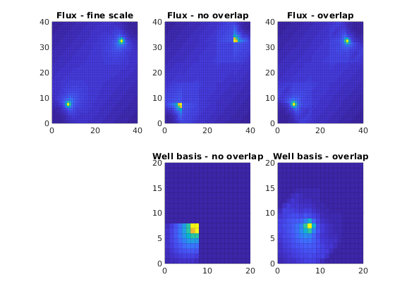
Multiscale Pressure Solver Speed up:
Generated from speedUpMSExample.m
The implementation of the multiscale method in MRST is meant to be flexible and is therefore not optimized when it comes to speed. Here we demonstrate how we can speed up the multiscale pressure solver considerably by preassembling the basis matrix and precompute values used in the multiscale pressure solver. This is particularly useful for 2-phase problems where we repeatedly solve the pressure and the transport equation because the preassembly only needs to be done once. In this demo we solve the single-phase pressure equation (i.e. only one pressure step)
for a Cartesian grid with isotropic, homogeneous permeability. This example is built upon the flow-solver tutorial simpleWellExampleMS.html. It is recommended that you look at this tutorial first.
mrstModule add coarsegrid mimetic msmfem incomp
Define the model and set data
We construct the Cartesian grid, set the permeability to 100 mD, and use a single-phase fluid with density 1000 kg/m^3 and viscosity 1 cP.
nx = 15; ny = 15; nz = 15;
Nx =  3; Ny =  3; Nz = 3;
verbose   = false;
G         = cartGrid([nx ny nz]);
G         = computeGeometry(G);
rock.perm = repmat(100*milli*darcy, [G.cells.num, 1]);
fluid     = initSingleFluid('mu' ,    1*centi*poise     , ...
                            'rho', 1000*kilogram/meter^3);
Set two wells, one vertical and one horizontal.
W = verticalWell([], G, rock, nx, ny, 1:nz,            ...
                 'InnerProduct', 'ip_simple', ...
                'Type', 'rate', 'Val', 1*meter^3/day, ...
                'Radius', .1, 'Name', 'I', 'Comp_i', 1);
W = addWell(W, G, rock, 1:nx, 'Type','bhp', ...
            'InnerProduct', 'ip_simple', ...
            'Val', 1*barsa, 'Radius', .1, 'Dir', 'x', ...
            'Name', 'P', 'Comp_i', 0);
Set up solution structures
Here we need three solution structures, one for each simulator to hold the solutions on the grid and in the wells.
xRef = initState(G, W, 0, 1);
xMs  = xRef;
xMs_speed  = xRef;
Partition the grid
We partition the fine grid into coarse blocks.
p = partitionUI(G, [Nx, Ny, Nz]);
p = processPartition(G, p);
Generate the coarse-grid structure
CG = generateCoarseGrid(G, p, 'Verbose', verbose);
Assemble linear systems
First we compute the inner product to be used in the fine-scale and coarse-scale linear systems. Then we generate the coarse-scale system.
gravity off
S  = computeMimeticIP(G, rock, 'Verbose', verbose);

mu  = fluid.properties(xMs);
kr  = fluid.relperm(ones([G.cells.num, 1]), xMs);
mob = kr ./ mu;

CS  = generateCoarseSystem(G, rock, S, CG, mob, 'Verbose', verbose);
Precompute and preassemble to speed up multiscale
Preassemble multiscale basis matrix and precompute grid values used in the speeded up version of the multiscale pressure solver.
[CGspeed, CSspeed] = speedUpMS(G, CG, CS, S.type);
Display the difference between GS/CGspeed and CS/CSspeed
display(CG);
display(CGspeed);

display(CS);
display(CSspeed);
CG =

  struct with fields:

        cells: [1×1 struct]
        faces: [1×1 struct]
    partition: [3375×1 double]
...
Plot basis function matrix
Pick a 2D slice of the grid and display velocity basis matrix for the cells in the 2D slice
% 2D slice:
fineCells = (nx*nx*floor(nz/2)+1):(nx*nx*floor(nz/2+1));

% Find cellfaces of fineCells, each cell has 6 cellfaces
cellFaces = mcolon((fineCells-1)*6 +1 , fineCells*6);
clf
subplot(2,2,1)
   plotCellData(G, mod(p,5), (1:G.cells.num)');
   axis equal tight; view(3)
   title('Coarse grid partition')

subplot(2,2,3)
   outlineCoarseGrid(G, p, 'FaceColor', 'none', 'EdgeAlpha', 0.2);
   axis equal tight; view(3);
   plotCellData(G, mod(p(fineCells),5), fineCells);
   title('2D slice with coarse grid indicated')

subplot(2,2,[2 4])
   spy(CSspeed.Bv(cellFaces,:));
   title('Velocity basis matrix for cells in 2D slice');
   ylabel('Fine cellface')
   xlabel('Coarse cellface')
   set(gca, 'XTick', []);
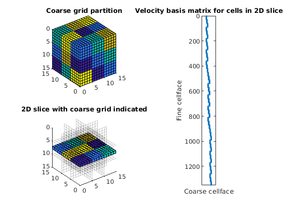
Then, we assemble the well systems for the fine and the coarse scale.
W = generateCoarseWellSystem(G, S, CG, CS, mob, rock, W);
Solve the global flow problems and check time consumption
tic
xRef = incompMimetic(xRef, G, S, fluid, 'wells', W, 'Solver', S.type);
t_fine = toc;

tic
xMs  = solveIncompFlowMS(xMs , G, CG, p, S, CS, fluid, 'wells', W, ...
                         'Solver', S.type);
t_ms_org = toc;

tic
xMs_speed  = solveIncompFlowMSSpeedUp(xMs_speed , G, CGspeed, p, S, ...
                                      CSspeed, fluid, 'wells', W,   ...
                                      'Solver', S.type);
t_ms_speed = toc;
Report time consumption for multiscale pressure solver
disp('* Time consumption of multiscale solvers compared to fine scale: *')
disp(['Multiscale original: ', num2str(t_ms_org/t_fine), ' %']);
disp(['Multiscale speedUp:  ', num2str(t_ms_speed/t_fine), ' %' ]);
* Time consumption of multiscale solvers compared to fine scale: *
Multiscale original: 0.32318 %
Multiscale speedUp:  0.38328 %
Multiscale Pressure Solver: Dynamic update of basis functions
Generated from updateBasisMSExample.m
Consider a two-phase oil-water problem. Solve the two-phase pressure equation

where v is the Darcy velocity (total velocity) and lambda is the mobility, which depends on the water saturation S. The saturation equation (conservation of the water phase) is given as:
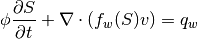
where phi is the rock porosity, f is the Buckley-Leverett fractional flow function, and q_w is the water source term. As the transport solution advances we update the basis functions if the mobility changes more than a given tolerance. After the simulation is done we compare the fine scale and coarse scale saturation profiles.
mrstModule add coarsegrid mimetic msmfem incomp
Define and visualize the model
We construct the Cartesian grid, set the permeability to 100 mD, and use the default single-phase fluid with unit viscosity
cellDims  = [40, 40, 10];
verbose   = mrstVerbose;
G         = cartGrid(cellDims, cellDims);
G         = computeGeometry(G);
rock.perm = repmat(100*milli*darcy, [G.cells.num, 1]);
rock.poro = 0.3*ones(G.cells.num,1);
fluid     = initCoreyFluid('mu' , [   1,  10]*centi*poise     , ...
                           'rho', [1000, 700]*kilogram/meter^3, ...
                           'n'  , [   2,   2], ...
                           'sr' , [ 0.2, 0.2], ...
                           'kwm', [   1,   1]);

% Set two wells, one vertical and one horizontal
W = struct([]);
W = verticalWell(W, G, rock, 40, 40, 1:10, ...
                 'InnerProduct', 'ip_simple', ...
                 'Type', 'rate', 'Val', 1*meter^3/day, ...
                 'Radius', .1, 'Name', 'I');
W = addWell(W, G, rock, 1:40, 'Type','bhp', ...
            'InnerProduct', 'ip_simple', ...
            'Val', 0, 'Radius', .1, 'Dir', 'x', 'Name', 'P');

% Visualize the model
figure;
plotGrid(G, 'FaceColor', 'none', 'EdgeColor', [0.65, 0.65, 0.65]);
plotWell(G, W, 'radius', 0.1, 'color', 'r');
view(3); axis equal tight off

Set up solution structures
Here we need four solution structures, two for each simulator to hold the solutions on the grid and in the wells, respectively.
xRef = initState(G, W, 0);
xMs  = initState(G, W, 0);
Partition the grid
We partition the fine grid into a regular 5-by-5-by-2 coarse grid in index space so that each coarse block holds 8-by-8-by-5 fine cells. The resulting vector p has one entry per fine-grid cell giving the index of the corresponding coarse block. After the grid is partitioned in index space, we postprocess it to make sure that all blocks consist of a connected set of fine cells. This step is superfluous for Cartesian grids, but is required for grids that are only logically Cartesian (e.g., corner-point and other mapped grids that may contain inactive or degenerate cells).
p  = partitionUI(G, [5, 5, 2]);
p  = processPartition(G, p);

figure;
plotCellData(G,mod(p,2)); view(3); axis equal tight off

CG = generateCoarseGrid(G, p, 'Verbose', verbose);

S  = computeMimeticIP(G, rock, 'Verbose', verbose);

mu  = fluid.properties(xMs);
totmob = @(s) (sum(bsxfun(@rdivide, fluid.relperm(s), mu),2));
mob = totmob(xMs.s);
CS = generateCoarseSystem (G, rock, S, CG, mob, ...
                           'Verbose', verbose);

W = generateCoarseWellSystem(G, S, CG, CS, ones([G.cells.num, 1]), rock, W);

xRef = incompMimetic    (xRef, G, S, fluid, 'wells', W);
xMs  = solveIncompFlowMS(xMs, G, CG, p, S, CS, fluid, 'wells', W);
Warning: Inconsistent Number of Phases. Using 2 Phases (=min([3, 2, 2])).
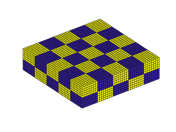
Report initial state of reservoir
subplot(2,1,1), cla
   plotCellData(G, convertTo(xRef.pressure(1:G.cells.num), barsa));
   title('Initial pressure fine'), view(3)

subplot(2,1,2), cla
   plotCellData(G, convertTo(xRef.pressure(1:G.cells.num), barsa));
   title('Initial pressure MS'), view(3)

dp = @(x) num2str(convertTo(x(1).pressure, barsa));
disp(['DeltaP - Fine: ', dp(xRef.wellSol)]);
disp(['DeltaP - Ms:   ', dp(xMs .wellSol)]);
DeltaP - Fine: 3.7478
DeltaP - Ms:   3.7875
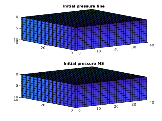
Transport loop
We solve the two-phase system using a sequential splitting in which the pressure and fluxes are computed by solving the flow equation and then held fixed as the saturation is advanced according to the transport equation. This procedure is repeated for a given number of time steps (here we use 15 equally spaced time steps). The error introduced by this splitting of flow and transport can be reduced by iterating each time step until e.g., the residual is below a certain user-prescribed threshold (this is not done herein).
T      = 500*day();
dT     = T/20;
dTplot = 100*day();  % plot only every 100th day
N      = fix(T/dTplot);
pv     = poreVolume(G,rock);
t  = 0; plotNo = 1; hi = 'Ms solution '; he = 'Updated blocks';
e = []; pi = []; pe = [];


while t < T,

   mobOld = mob;

   xRef  = explicitTransport(xRef , G, dT, rock, fluid, 'wells', W);
   xMs  = explicitTransport(xMs , G, dT, rock, fluid, 'wells', W);
   % Check for inconsistent saturations
   s = [xRef.s(:,1); xMs.s(:,1)];
   assert(max(s) < 1+eps && min(s) > -eps);

   % Update solution of pressure equation.
   xRef = incompMimetic    (xRef, G, S, fluid, 'wells', W);
   xMs  = solveIncompFlowMS(xMs , G, CG, p, S, CS, fluid, 'wells', W);

   % Check if we need to update basis functions
   mob = totmob(xMs.s);
   [CS, faces] = updateBasisFunc(S, CS, G, CG, rock, mob, ...
                                 'mobOld', mobOld, 'mobTol', 0);

   % find which blocks have been updated (use for ploting)
   updateBlocks = false([CG.cells.num + 1, 1]);
   updateBlocks(CG.faces.neighbors(faces, :) + 1) = true;
   updateBlocs(1) = false;
   fineCells = updateBlocks(CG.partition + 1);

   % Measure water saturation in production cells in saturation
   e = [e; sum(abs(xRef.s(:,1) - xMs.s(:,1)).*pv)/sum(pv)]; %#ok
   pe = [pe; xRef.s(W(2).cells,1)' ];                 %#ok
   pi = [pi; xMs.s(W(2).cells,1)'];                 %#ok

   % Increase time and continue if we do not want to plot saturations
   t = t + dT;

   % Plot updated blocks and saturation of multiscale
   heading = [num2str(convertTo(t,day)),  ' days'];

   subplot(2, 1, 1),
   cla
   plotGrid(G, 'faceColor', 'none', 'EdgeAlpha', 0.125);
   plotCellData(G, mod(CG.partition(fineCells), 3), ...
                find(fineCells), 'EdgeAlpha', 0.125);
   view(3), axis equal off, title(he)

   subplot(2, 1, 2),
   cla
   plotCellData(G, xMs.s(:,1), 'EdgeAlpha', 0.125);
   view(3), axis equal off, title([hi, heading])

   drawnow
end
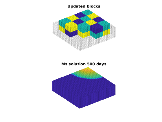
Compare multiscale saturation against fine scale plot output
f = figure;

subplot(2,1,1)
   plotCellData(G, xRef.s(:,1), 'EdgeAlpha', 0.125);
   title('Saturation Fine')
   view(3), camproj perspective, axis tight equal, camlight headlight
   caxis([0 1]); colorbar

subplot(2,1,2)
   plotCellData(G, xMs.s(:,1), 'EdgeAlpha', 0.125);
   title('Saturation Coarse')
   view(3), camproj perspective, axis tight equal, camlight headlight
   caxis([0 1]); colorbar