`optimization`¶

The optimization module contains routines for solving optimal control problems with (forward and adjoint) solvers based on the automatic differentiation framework found in ad-core and ad-blackoil. The module contains a quasi-Newton optimization routine using BFGS-updated Hessians, but can easily be set up to use any (non-MRST) optimization code.

Objective functions¶

Contents¶: Files matchObservedOW - Compute mismatch-function NPVBlackOil - Compute net present value of a schedule with well solutions NPVOW - Compute net present value of a schedule with well solutions NPVOWPolymer - Compute net present value of a schedule with well solutions

NPVBlackOil(G, wellSols, schedule, varargin)¶: Compute net present value of a schedule with well solutions

NPVOW(G, wellSols, schedule, varargin)¶: Compute net present value of a schedule with well solutions

NPVOWPolymer(G, wellSols, schedule, varargin)¶: Compute net present value of a schedule with well solutions

matchObservedOW(G, wellSols, schedule, observed, varargin)¶: Compute mismatch-function

Utilities¶

Optimization¶

Contents¶

OPTIM

Files: argmaxCubic - find max of cubic polynomial through p1, p2 lineSearch - lineSearch – helper function which performs line search based on unitBoxBFGS - Iterative line search optimization using BFGS intended for scaled

argmaxCubic(p1, p2)¶: find max of cubic polynomial through p1, p2 shift values:

lineSearch(u0, v0, g0, d, f, c, opt)¶

lineSearch – helper function which performs line search based on Wolfe-conditions.

SYNOPSIS: [u, v, g, info] = lineSearch(u0, v0, g0, d, f, c, opt)

PARAMETERS: u0 : current control vector v0 : current objective value g0 : current gradient d : search direction, returns an error unless d’*g0 > 0 f : objective function s.t. [v,g] = f(u) c : struct with linear inequality and equality constraints opt: struct of parameters for line search

RETURNS: u : control vector found along d v : objective value for u g : gradient for u info : struct containing fields:

flag : 1 for success (Wolfe conditions satisfied)

-1 max step-length reached without satisfying Wolfe-conds -2 line search failed in maxIt iterations (returns most recent control without further considerations)

step : step-length nits : number of iterations used

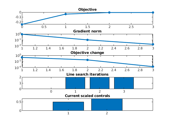
unitBoxBFGS(u0, f, varargin)¶

Iterative line search optimization using BFGS intended for scaled problems, i.e., 0<=u<=1 and f~O(1)

SYNOPSIS: [v, u, history] = unitBoxBFGS(u0, f, opt)

Contents¶

UTILS

Files: control2schedule - Convert control vector u to schedule evalObjective - Objective (and gradient) evaluation function based on input control vector u initSimpleScaledADIFluid - version of initSimpleScaledADIFluid with additional relperm scaling scaleConstraints - Linear constraint scaling schedule2control - Convert schedule to control vector setupConstraints - Setup linear constraints for scaled problem. Assumes linConst applies to

control2schedule(u, schedule, scaling)¶: Convert control vector u to schedule

evalObjective(u, obj, state0, model, schedule, scaling)¶: Objective (and gradient) evaluation function based on input control vector u

initSimpleScaledADIFluid(varargin)¶: version of initSimpleScaledADIFluid with additional relperm scaling

scaleConstraints(linConst, scaling)¶: Linear constraint scaling

schedule2control(schedule, scaling)¶: Convert schedule to control vector

setupConstraints(linConst, schedule, scaling)¶: Setup linear constraints for scaled problem. Assumes linConst applies to all control steps.

Examples¶

Optimize NPV for a simple faulted model¶

Generated from optimizeFaultedModel.m

This example covers the steps for setting up and running a simulation-based optimization problem.

Construct faulted grid, and populate with layered permeability field¶

mrstModule add ad-core ad-blackoil ad-props optimization

grdecl = makeModel3([20, 20, 4], [500, 500, 8]*meter);
G = processGRDECL(grdecl);
G = computeGeometry(G);

% Set up permeability based on K-indices
[I, J, K] = gridLogicalIndices(G);

px       = 100*milli*darcy*ones(G.cells.num,1);
px(K==2) = 500*milli*darcy;
px(K==3) = 50*milli*darcy;

% Introduce anisotropy by setting K_x = 5*K_z.
perm = [px, px, 0.1*px];
rock = makeRock(G, perm, 0.2);

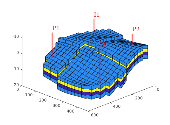
Define wells¶

We define two vertical producers and two vertical injectors. Rates correspond to one reservoir pore volume injected during 640 days

simTime = 640*day;
pv = poreVolume(G, rock);
injRate = 1*sum(pv)/simTime;

% Place wells
[nx, ny] = deal(G.cartDims(1), G.cartDims(2));
ppos = [nx-2, 4; 4   , ny-4];
ipos = [4   , 5; nx-3, ny-3];
offset = 5;
W = [];
% Injectors
W = verticalWell(W, G, rock, ipos(1,1), ipos(1,2), [], 'sign', 1,...
                'Name', 'I1', 'comp_i', [1 0], 'Val', injRate/2, 'Type', 'rate');

W = verticalWell(W, G, rock, ipos(2,1), ipos(2,2), [], 'sign', 1, ...
                'Name', 'I2', 'comp_i', [1 0], 'Val', injRate/2, 'Type', 'rate');
% Producers
W = verticalWell(W, G, rock, ppos(1,1), ppos(1,2), [], 'sign', -1, ...
                'Name', 'P1', 'comp_i', [0 1], 'Val', -injRate/2, 'Type', 'lrat');
W = verticalWell(W, G, rock, ppos(2,1), ppos(2,2), [], 'sign', -1, ...
                'Name', 'P2', 'comp_i', [0 1], 'Val', -injRate/2, 'Type', 'lrat');
figure,
plotCellData(G, log(rock.perm(:,1)));
plotWell(G, W), view([1 1 1])

Warning: Reference depth for well BHP in well 'I1' is set below well's top-most
reservoir connection
Warning: Reference depth for well BHP in well 'P2' is set below well's top-most
reservoir connection

Define base schedule¶

We set up 4 control-steps each 160 days. We explicitly set shorter time steps during start.

ts = { [1 2 5 7 10 15 20 20 20 20 20 20]'*day, ...
                      repmat(160/7, 7, 1)*day, ...
                      repmat(160/7, 7, 1)*day, ...
                      repmat(160/7, 7, 1)*day};

numCnt = numel(ts);
[schedule.control(1:numCnt).W] = deal(W);
schedule.step.control = rldecode((1:4)', cellfun(@numel, ts));
schedule.step.val     = vertcat(ts{:});

Set fluid properties (slightly compressible oil)¶

fluid = initSimpleADIFluid('mu',    [.3, 5, 0]*centi*poise, ...
                           'rho',   [1000, 700, 0]*kilogram/meter^3, ...
                           'n',     [2, 2, 0]);
c = 1e-5/barsa;
p_ref = 300*barsa;
fluid.bO = @(p) exp((p - p_ref)*c);

Initialize model and run base-case simulation¶

model  = TwoPhaseOilWaterModel(G, rock, fluid);
state0 = initResSol(G, p_ref, [0 1]);
schedule_base = schedule;
[wellSols_base, states_base] = simulateScheduleAD(state0, model, schedule_base);

Solving timestep 01/33:                               -> 1 Day
Solving timestep 02/33: 1 Day                         -> 3 Days
Solving timestep 03/33: 3 Days                        -> 8 Days
Solving timestep 04/33: 8 Days                        -> 15 Days
Solving timestep 05/33: 15 Days                       -> 25 Days
Solving timestep 06/33: 25 Days                       -> 40 Days
Solving timestep 07/33: 40 Days                       -> 60 Days
Solving timestep 08/33: 60 Days                       -> 80 Days
...

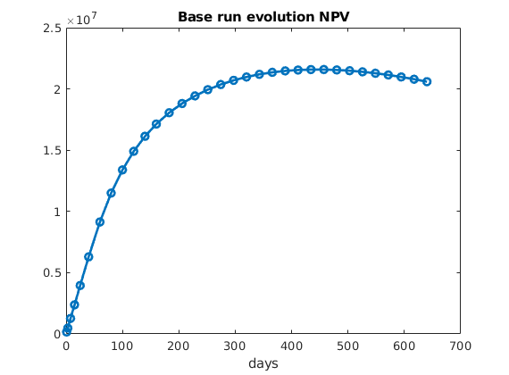
Set prices ($/stb), discount rate (/year) and plot evolutiuon of NPV¶

npvopts     = {'OilPrice',             60.0 , ...
               'WaterProductionCost',   7.0 , ...
               'WaterInjectionCost',    7.0 , ...
               'DiscountFactor',        0.1 };
v_base  = NPVOW(G, wellSols_base, schedule_base, npvopts{:});
v_base  = cell2mat(v_base);
t_base  = cumsum(schedule_base.step.val);
figure, plot(convertTo(t_base,day), cumsum(v_base), '-o', 'LineWidth', 2);
title('Base run evolution NPV'), xlabel('days')

Set up box limits for scaling and define function evaluation handle¶

li = [  10, 300]/day;  % Injector limits
lp = [-300, -10]/day;  % Producer limits
scaling.boxLims = [li;li;lp;lp];  % control scaling
scaling.obj     = sum(v_base);    % objective scaling
% Get initial scaled controls
u_base = schedule2control(schedule_base, scaling);
% Define objective function with above options
obj = @(wellSols, schedule, varargin)NPVOW(G, wellSols, schedule, varargin{:}, npvopts{:});
% Get function handle for objective evaluation
f = @(u)evalObjective(u, obj, state0, model, schedule, scaling);

Define linear equality and inequality constraints, and run optimization¶

Constraints are applied to all control steps such for each step i, we enforce linEq.A*u_i = linEq.b linIneq.A*u_i = linIneq.b All rates should add to zero to preserve reservoir pressure (I1, I2, P1, P2)

linEq = struct('A', [1 1 1 1], 'b', 0);
% We also impose a total water injection constraint <= 500/day
linIneq = struct('A', [1 1 0 0], 'b', 500/day);
% Constraints must be scaled!
linEqS   = setupConstraints(linEq,   schedule, scaling);
linIneqS = setupConstraints(linIneq, schedule, scaling);
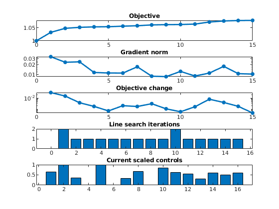
% Run optimization with default options
[v, u_opt, history] = unitBoxBFGS(u_base, f, 'linEq', linEqS, 'linIneq', linIneqS);

Solving timestep 01/33:                               -> 1 Day
Solving timestep 02/33: 1 Day                         -> 3 Days
Solving timestep 03/33: 3 Days                        -> 8 Days
Solving timestep 04/33: 8 Days                        -> 15 Days
Solving timestep 05/33: 15 Days                       -> 25 Days
Solving timestep 06/33: 25 Days                       -> 40 Days
Solving timestep 07/33: 40 Days                       -> 60 Days
Solving timestep 08/33: 60 Days                       -> 80 Days
...

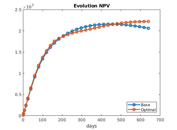
Evaluate evolution of NPV for optimal schedule and compare with base¶

chedule_opt = control2schedule(u_opt, schedule, scaling);
[wellSols_opt, states_opt] = simulateScheduleAD(state0, model, schedule_opt);
v_opt  = NPVOW(G, wellSols_opt, schedule_opt, npvopts{:});
v_opt  = cell2mat(v_opt);
t_opt  = cumsum(schedule_opt.step.val);
figure, plot(convertTo([t_base, t_opt],day), cumsum([v_base, v_opt]), '-o', 'LineWidth', 2);
title('Evolution NPV'), legend('Base', 'Optimal', 'Location', 'se'), xlabel('days')

% <html>
% <p><font size="-1

Solving timestep 01/33:                               -> 1 Day
Solving timestep 02/33: 1 Day                         -> 3 Days
Solving timestep 03/33: 3 Days                        -> 8 Days
Solving timestep 04/33: 8 Days                        -> 15 Days
Solving timestep 05/33: 15 Days                       -> 25 Days
Solving timestep 06/33: 25 Days                       -> 40 Days
Solving timestep 07/33: 40 Days                       -> 60 Days
Solving timestep 08/33: 60 Days                       -> 80 Days
...

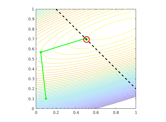
Gradient-based search for optimium of a quadratic function on unit square¶

Generated from optimizeQuad.m

mrstModule add ad-core optimization
% Define test-function parameters:
opts = {'th', pi/10, ...
        'rx', 4 ,    ...
        'ry', 1 ,    ...
        'x0', .8,    ...
        'y0', .8};
% Compute function value at mesh-points for subsequent contour-plots
[X,Y] = meshgrid(0:.01:1, 0:.01:1);
Z = testFunction(X,Y, opts{:});
% Function handle:
f = @(u)testFunction(u(1),u(2), opts{:});
% Initial guess:
u0 = [.1, .1]';

% Linear inequality constaint in addition to box: y< -x + 1.2
le = struct('A', [1 1], 'b', 1.2);

Optimize using BFGS:¶

v1,u1,hst1] = unitBoxBFGS(u0, f, 'useBFGS', true, ...
                                   'wolfe1', 1e-3, ...
                                   'wolfe2',  0.5,  ...
                                   'linIneq',  le);


% Gather evolution of control-vector:
p1 = horzcat(hst1.u{:})';
% Plot contour of objective and evolution of controls
figure(11),hold on
contour(X,Y,Z,-.5:.011:0);
plot(p1(:,1),p1(:,2),'.-g','LineWidth', 2, 'MarkerSize', 20)
plot(p1(end,1),p1(end,2),'or','LineWidth', 2, 'MarkerSize', 15)
% Plot linear inequality constraint
x = 0:1; y = -(le.A(1)*x - le.b)/le.A(2);
plot(x, y, '--k','LineWidth', 2)
axis equal, axis tight, box on
axis equal, axis tight, box on, axis([0 1 0 1])

% <html>
% <p><font size="-1

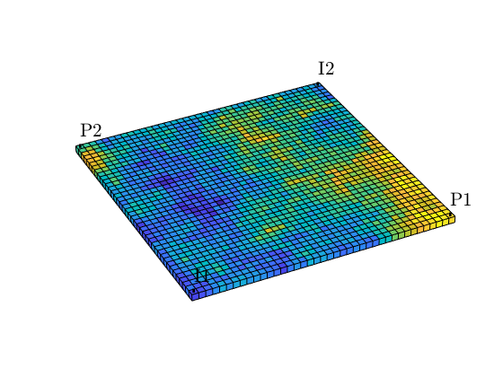
NPV - analysis for a simple 2D model¶

Generated from analyseModel2D.m

In this example we consider a simple 2D oil-water model. The main purpose is a comparison between a base simulation and an optimal NPV simulation as obtained by the script ‘optimizeModel2D’. The optimization will run only the first time this script is called, as the optimal schedule will be saved and loaded at next execution. The script is intended for MATLAB-Publish, and it is advised to set Max # of output lines in Publish settings to 1.

% Load required modules
mrstModule add ad-core ad-blackoil ad-props optimization spe10

% Start by running script in utils-directory to set up example model
setupModel2D
% Plot grid with x-permeability and wells:
close all
figure, plotCellData(G, log(rock.perm(:,1)));
plotWell(G, W, 'Fontsize', 16, 'Color', 'k');
axis off, axis equal, axis tight, camproj perspective, view([-1 -2 1.5]);

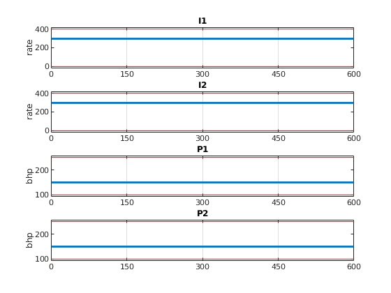
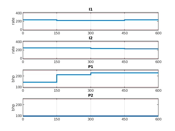
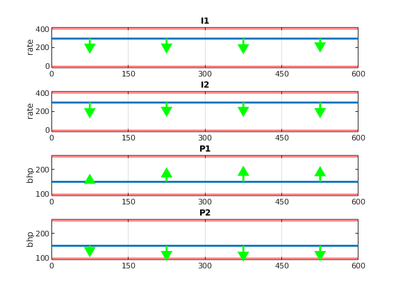
Base and optimal schedules¶

% Check if we need to run optimization, if not, load optimal schedule:
try
    load('schedule_opt');
catch
    fprintf('Running optimization, this may take a few minutes ...\n')
    optimizeModel2D;
end
close all
% Display base and optimal schedule:
li = [0 400]/day;        % Injector limits
lp = [100 250]*barsa;    % Producer limits
figure,
plotSchedules(schedule, 'singlePlot', true, 'boxConst', [li;li;lp;lp] )
figure,
plotSchedules(schedule_opt, 'singlePlot', true, 'boxConst', [li;li;lp;lp] )

Run forward simulation for base and optimal schedule¶

% Create model-object of class TwoPhaseOilWaterModel
model  = TwoPhaseOilWaterModel(G, rock, fluid);
% Set initial state and run simulations:
state0 = initResSol(G, 200*barsa, [0, 1]);
[wellSols, states]         = simulateScheduleAD(state0, model, schedule);
[wellSols_opt, states_opt] = simulateScheduleAD(state0, model, schedule_opt);

Solving timestep 01/37:                  -> 1 Day
Solving timestep 02/37: 1 Day            -> 2 Days
Solving timestep 03/37: 2 Days           -> 5 Days
Solving timestep 04/37: 5 Days           -> 10 Days
Solving timestep 05/37: 10 Days          -> 15 Days
Solving timestep 06/37: 15 Days          -> 25 Days
Solving timestep 07/37: 25 Days          -> 35 Days
Solving timestep 08/37: 35 Days          -> 45 Days
...

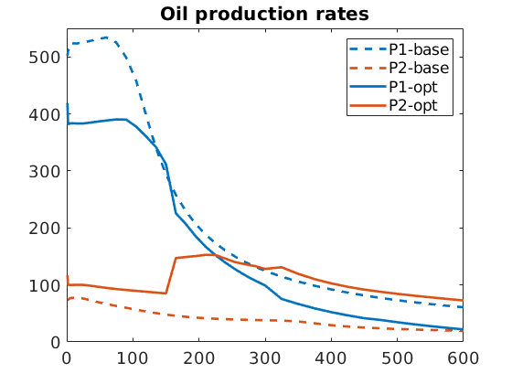
Plot oil and water production for producer wells for both scenarios:

dtime = schedule.step.val/day;
time  = cumsum(dtime);
qOs     = - getWellOutput(wellSols, 'qOs', 3:4);
qOs_opt = - getWellOutput(wellSols_opt, 'qOs', 3:4);
figure, plot(time, qOs*day, '--', 'LineWidth', 2)
hold on,
ax = gca;
if ~isnumeric(ax)
    ax.ColorOrderIndex = 1;
end

plot(time, qOs_opt*day, '-'  ,'LineWidth', 2)
axis([0 600 0 550]), set(gca, 'FontSize', 14)
legend([W(3).name, '-base'] , [W(4).name, '-base'], [W(3).name, '-opt'] , [W(4).name, '-opt'] )
title('Oil production rates')

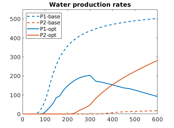
qWs     = - getWellOutput(wellSols, 'qWs', 3:4);
qWs_opt = - getWellOutput(wellSols_opt, 'qWs', 3:4);
figure, plot(time, qWs*day, '--','LineWidth', 2)
hold on,
ax = gca;
if ~isnumeric(ax)
    ax.ColorOrderIndex = 1;
end

plot(time, qWs_opt*day, '-'  ,'LineWidth', 2)
axis([0 600 0 550]), set(gca, 'FontSize', 14)
legend([W(3).name, '-base'] , [W(4).name, '-base'], [W(3).name, '-opt'] , ...
       [W(4).name,  '-opt'], 'Location', 'northwest');
title('Water production rates')

Problem economics:¶

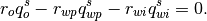
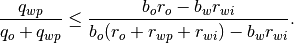
We here define economic parameters, and analyse net cash flow and NPV. We define the critical water cut to be the highest water cut resulting in a non-negative net cash-flow under assumption of reservoir volume balance, i.e the water cut for wich we have

$r_oq_o^s - r_{wp}q_{wp}^s - r_{wi}q_{wi}^s = 0.$

Combining with reservoir volume balance, we obtain:

$\frac{q_{wp}}{q_o+q_{wp}}\leq\frac{b_or_o-b_wr_{wi}}{b_o(r_o+r_{wp}+r_{wi})-b_wr_{wi}}.$

% Revenue, costs and discount rate
d   = 0.05;    % yearly discount factor
ro  = 60;      % oil revenue/price ($/stb)
rwp =  6;      % water production handling costs ($/stb)
rwi =  6;      % water injection cost ($/stb)
npvopts = {'OilPrice',             ro , ...
           'WaterProductionCost', rwp , ...
           'WaterInjectionCost',  rwi , ...
           'DiscountFactor',        d};

% Compute critical water-cut value at 200 bar:
[bw, bo] = deal(fluid.bW(200*barsa), fluid.bO(200*barsa));
wcut_crit = (bo*ro-bw*rwi)/(bo*(ro+rwp+rwi)-bw*rwi);
fprintf('Maximal economic water cut: %4.3f\n', wcut_crit)

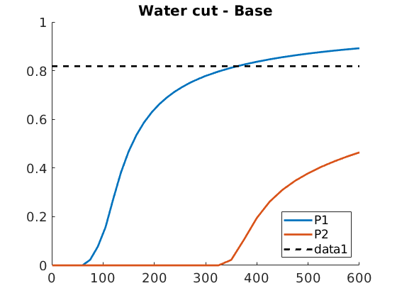
% Plot water-cut for each producer and critical water-cut:
figure, hold on, plot(time, qWs./(qOs+qWs), 'LineWidth', 2)
axis([0 600 0 1]), set(gca, 'FontSize', 14)
legend(W(3).name, W(4).name, 'Location', 'southeast')
plot([0 600], wcut_crit*[1 1], '--k', 'LineWidth', 2);
title('Water cut - Base')
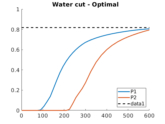
figure, hold on, plot(time, qWs_opt./(qOs_opt+qWs_opt), 'LineWidth', 2)
axis([0 600 0 1]), set(gca, 'FontSize', 14)
legend(W(3).name, W(4).name, 'Location', 'southeast')
plot([0 600], wcut_crit*[1 1], '--k', 'LineWidth', 2);
title('Water cut - Optimal')

Maximal economic water cut: 0.818

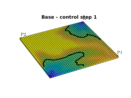
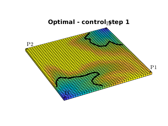
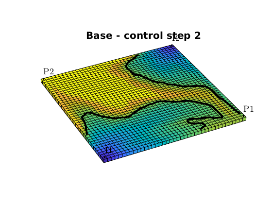
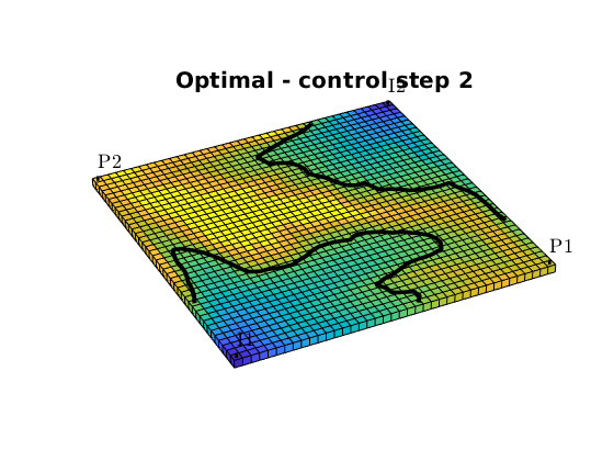
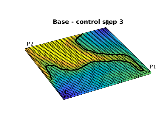
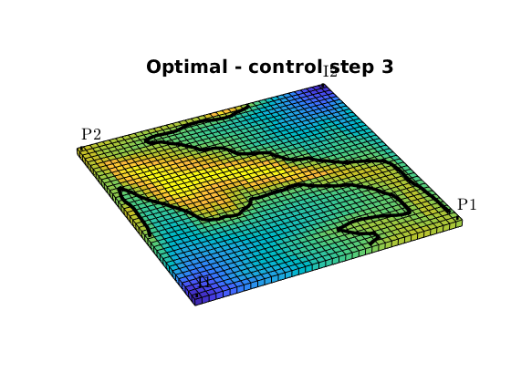
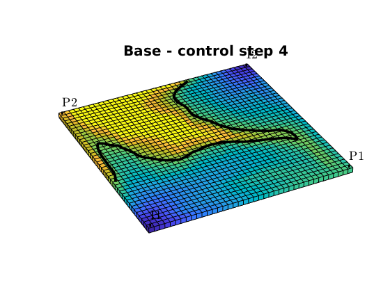
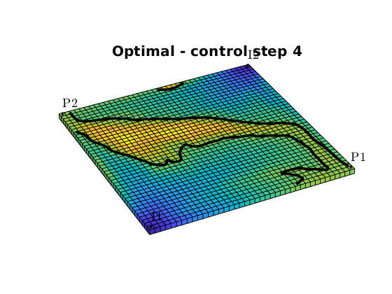
Fractional flow contours¶

We can also plot fractional flow in the reservoir together with a contour of of the critical water cut. We chose the reservoir states at the end of each of the four control-steps, and compare economic regions of the reservoir:

[~,n] = rlencode(schedule.step.control);
for k = 1:4
    figure,
    fracFlowContours(G, W, states(sum(n(1:k))), fluid, wcut_crit, 'LineWidth', 3, 'color', 'k');
    title(['Base - control step ', num2str(k)])
    figure,
    fracFlowContours(G, W, states_opt(sum(n(1:k))), fluid, wcut_crit, 'LineWidth', 3, 'color', 'k');
    title(['Optimal - control step ', num2str(k)])
end

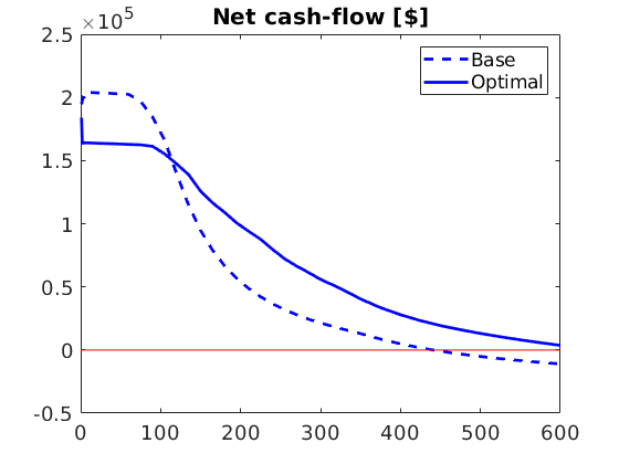
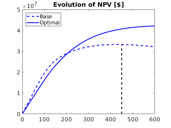
Compute and plot net cashflow and NPV¶

Net present value (NPV) is the sum (integral) of discounted net cash flows. Hence, for positive cash-flows, NPV is increasing.

close all
vals     = cell2mat(NPVOW(G, wellSols, schedule, npvopts{:}));
vals_opt = cell2mat(NPVOW(G, wellSols_opt, schedule_opt, npvopts{:}));
% Plot discounted net cashflow $/day:
figure,  plot(time, vals./dtime, '--b','LineWidth', 2);
hold on, plot(time, vals_opt./dtime, '-b','LineWidth', 2);
line([0 600], [0 0], 'color', 'r'), set(gca, 'FontSize', 14)
title('Net cash-flow [$]'), legend('Base', 'Optimal')
% Find index of first occuring time > 10 days, where net cashflow becomes
% negative:
inx = find(and(vals<0, time>10), 1, 'first');

% Plot evolution of NPV and indicate peak value:
npv = cumsum(vals);
figure,  plot(time, cumsum(vals), '--b', 'LineWidth', 2);
hold on, plot(time, cumsum(vals_opt), '-b', 'LineWidth', 2);
plot([1 1]*time(inx), [0 npv(inx)], '--k', 'LineWidth', 2)
set(gca, 'FontSize', 14), title('Evolution of NPV [$]'),
legend('Base', 'Optimal', 'Location', 'northwest')

Visualize adjoint gradient for base simulation.¶

We compute the gradient by performing an adjoint simulation w.r.t to the NPV-objective.

bjh = @(tstep)NPVOW(G, wellSols, schedule, 'ComputePartials', true, 'tStep', tstep, npvopts{:});
g     = computeGradientAdjointAD(state0, states, model, schedule, objh);

% We visualize the obtained gradient in a shedule-plot. Actual gradient
% values are scaled for plotting purposes:
figure
plotSchedules(schedule, 'grad', g, 'singlePlot', true, 'boxConst', [li;li;lp;lp] )


% <html>
% <p><font size="-1

Solving reverse mode step 1 of 37
Solving reverse mode step 2 of 37
Solving reverse mode step 3 of 37
Solving reverse mode step 4 of 37
Solving reverse mode step 5 of 37
Solving reverse mode step 6 of 37
Solving reverse mode step 7 of 37
Solving reverse mode step 8 of 37
...

% optimizeModel2D - optimize NPV for example-model of this folder

mrstModule add ad-core ad-blackoil ad-props optimization spe10
setupModel2D

% Create model-object of class TwoPhaseOilWaterModel
model  = TwoPhaseOilWaterModel(G, rock, fluid);
% Set initial state and run simulation:
state0 = initResSol(G, 200*barsa, [0, 1]);

Set up box limits for scaling and define function evaluation handle¶

Generated from optimizeModel2D.m

li = [0 400]/day;        % Injector limits
lp = [100 250]*barsa;    % Producer limits
scaling.boxLims = [li;li;lp;lp];  % control scaling
scaling.obj     = 3.2e7;      % objective scaling
% Get initial scaled controls
u_base = schedule2control(schedule, scaling);
% Define objective function
d   = 0.05;    % yearly discount factor
ro  = 60;      % oil revenue/price ($/stb)
rwp =  6;      % water production handling costs ($/stb)
rwi =  6;      % water injection cost ($/stb)
npvopts = {'OilPrice',             ro , ...
           'WaterProductionCost', rwp , ...
           'WaterInjectionCost',  rwi , ...
           'DiscountFactor',        d};

obj = @(wellSols, schedule, varargin)NPVOW(G, wellSols, schedule, varargin{:}, npvopts{:});
% Get function handle for objective evaluation
f = @(u)evalObjective(u, obj, state0, model, schedule, scaling);

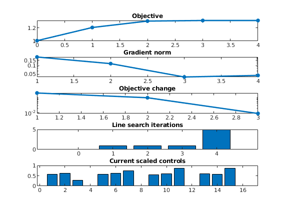
Run optimization with default options¶

v, u_opt, history] = unitBoxBFGS(u_base, f);
schedule_opt = control2schedule(u_opt, schedule, scaling);
pth = fullfile(mrstPath('optimization'), 'examples', 'model2D', 'schedule_opt.mat');
save(pth, 'schedule_opt')


% <html>
% <p><font size="-1

Solving timestep 01/37:                  -> 1 Day
Solving timestep 02/37: 1 Day            -> 2 Days
Solving timestep 03/37: 2 Days           -> 5 Days
Solving timestep 04/37: 5 Days           -> 10 Days
Solving timestep 05/37: 10 Days          -> 15 Days
Solving timestep 06/37: 15 Days          -> 25 Days
Solving timestep 07/37: 25 Days          -> 35 Days
Solving timestep 08/37: 35 Days          -> 45 Days
...

sensitivitiesModel2D - analyse sensitivity capabilities¶

Generated from sensitivitiesModel2D.m

mrstModule add ad-core ad-blackoil ad-props optimization spe10 mrst-gui

% Setup model -> grid, rock, schedule, fluid etc
setupModel2D

Reset fluid to include scaling:¶

fluid = initSimpleScaledADIFluid('mu',    [.3, 5, 0]*centi*poise, ...
                                 'rho',   [1000, 700, 0]*kilogram/meter^3, ...
                                 'n',     [2, 2, 0], ...
                                 'swl',   0.10*ones(G.cells.num,1), ...
                                 'swcr',  0.15*ones(G.cells.num,1), ...
                                 'sowcr', 0.12*ones(G.cells.num,1), ...
                                 'swu',   0.90*ones(G.cells.num,1));


% Create model-object of class TwoPhaseOilWaterModel
model_ref  = TwoPhaseOilWaterModel(G, rock, fluid);

% Set initial state and run simulation:
state0 = initResSol(G, 200*barsa, [.15, .85]);

% Set up a perturbed model with different pv and perm:
rock1 = rock;
rock1.perm = rock.perm*1.1;
model = TwoPhaseOilWaterModel(G, rock1, fluid);
model.operators.pv = model_ref.operators.pv.*0.8;

% run ref model
[ws_ref, states_ref, r_ref] = simulateScheduleAD(state0, model_ref, schedule);
% run model
[ws, states, r] = simulateScheduleAD(state0, model, schedule);

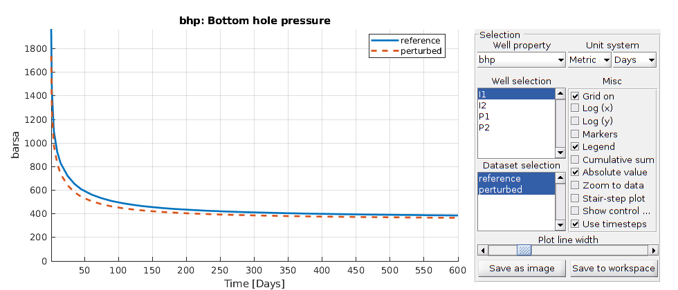
% plot well solutions for the two models
plotWellSols({ws_ref, ws}, {r_ref.ReservoirTime, r.ReservoirTime}, ...
            'datasetnames', {'reference', 'perturbed'})

Solving timestep 01/37:                  -> 1 Day
Solving timestep 02/37: 1 Day            -> 2 Days
Solving timestep 03/37: 2 Days           -> 5 Days
Solving timestep 04/37: 5 Days           -> 10 Days
Solving timestep 05/37: 10 Days          -> 15 Days
Solving timestep 06/37: 15 Days          -> 25 Days
Solving timestep 07/37: 25 Days          -> 35 Days
Solving timestep 08/37: 35 Days          -> 45 Days
...

setup misfit-function and run adjoint to get parameter sensitivities¶

setup weights for matching function, empty weight uses default (will produce function value of ~O(1) for 100% misfit). Only match rates in this example:

weighting =  {'WaterRateWeight',     [], ...
              'OilRateWeight',       [] , ...
              'BHPWeight',           0};

% compute misfit function value (first each summand corresonding to each time-step)
misfitVals = matchObservedOW(G, ws, schedule, ws_ref, weighting{:});
% sum values to obtiain scalar objective
misfitVal = sum(vertcat(misfitVals{:}));
fprintf('Current misfit value: %6.4e\n', misfitVal)

% setup (per time step) mismatch function handle for passing on to adjoint sim
objh = @(tstep)matchObservedOW(G, ws, schedule, ws_ref, 'computePartials', true, 'tstep', tstep, weighting{:});

% run adjoint to compute sensitivities of misfit wrt params
% choose parameters, get multiplier sensitivities except for endpoints
params      = {'porevolume', 'permeability', 'swl',   'swcr',  'sowcr', 'swu'};
paramTypes  = {'multiplier', 'multiplier',   'value', 'value', 'value', 'value'};

sens = computeSensitivitiesAdjointAD(state0, states, model, schedule, objh, ...
                                     'Parameters'    , params, ...
                                     'ParameterTypes', paramTypes);

Current misfit value: 9.9758e-05
Solving reverse mode step 1 of 37
Solving reverse mode step 2 of 37
Solving reverse mode step 3 of 37
Solving reverse mode step 4 of 37
Solving reverse mode step 5 of 37
Solving reverse mode step 6 of 37
Solving reverse mode step 7 of 37
...

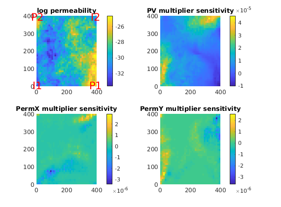
Plot sensitivities on grid:¶

figure,
subplot(2,2,1), plotCellData(G, log(rock.perm(:,1)), 'EdgeColor', 'none'), title('log permeability')
plotWellData(G, W);colorbar
subplot(2,2,2), plotCellData(G, sens.porevolume, 'EdgeColor', 'none'), colorbar,title('PV multiplier sensitivity');
subplot(2,2,3), plotCellData(G, sens.permx, 'EdgeColor', 'none'), colorbar,title('PermX multiplier sensitivity');
subplot(2,2,4), plotCellData(G, sens.permy, 'EdgeColor', 'none'), colorbar,title('PermY multiplier sensitivity');

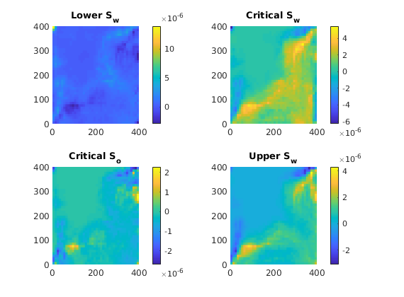
Rel-perm end-point sensitivities¶

figure,
nms = {'Lower S_w', 'Critical S_w', 'Critical S_o', 'Upper S_w'};
for k = 1:4
    subplot(2,2,k), plotCellData(G, sens.(params{k+2}), 'EdgeColor', 'none'), colorbar,title(nms{k});
end

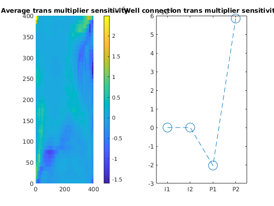
Run new adjoint to obtain transmissibility and well connection transmissibilitiy sensitivities¶

params      = {'transmissibility', 'conntrans'};
paramTypes  = {'multiplier', 'multiplier'};
sens = computeSensitivitiesAdjointAD(state0, states, model, schedule, objh, ...
                                     'Parameters'    , params, ...
                                     'ParameterTypes', paramTypes);

figure,
subplot(1,2,1), plotCellData(G,  cellAverage(G, sens.transmissibility), 'EdgeColor', 'none'), colorbar,title('Average trans multiplier sensitivity');
subplot(1,2,2), plot(sens.conntrans, '--o', 'MarkerSize', 14); title('Well connection trans multiplier sensitivity')
a = gca; a.XTick = 1:4;  a.XTickLabel = {W.name}; a.XLim; a.XLim = [.5 4.5];


model.fluid = initSimpleScaledADIFluid(model.fluid, 'swl', zeros(G.cells.num,1), ...
                                                    'swcr', zeros(G.cells.num,1), ...
                                                    'sowcr', zeros(G.cells.num,1), ...
                                                    'swu', ones(G.cells.num,1));
sens = computeSensitivitiesAdjointAD(state0, states, model, schedule, objh, ...
                                     'Parameters'    , {'swl', 'swcr', 'sowcr', 'swu'});

Solving reverse mode step 1 of 37
Solving reverse mode step 2 of 37
Solving reverse mode step 3 of 37
Solving reverse mode step 4 of 37
Solving reverse mode step 5 of 37
Solving reverse mode step 6 of 37
Solving reverse mode step 7 of 37
Solving reverse mode step 8 of 37
...