MRSTlogo_web_banner_light_thinner_Epi.png

Bravo Dome tutorial

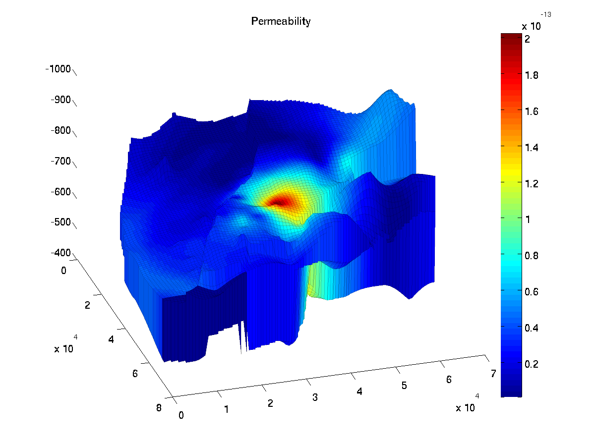
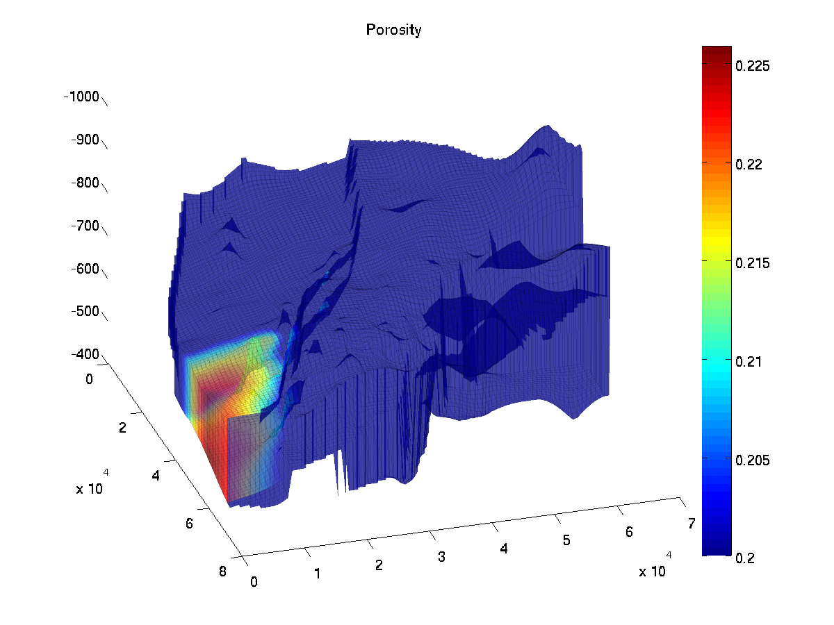
The Bravo Dome carbon dioxide gas field is located in northeast New Mexico. The Bravo Dome field covers approximately 3200 km^2. Production in 1989 was 3.2e9 cubic meter of gas from 272 wells. Cumulative production at the end of 1989 was 17e9 cubic meter. Estimated recoverable reserves are more than 283e9 cubic meter. The gas is 98-99% CO2. Most CO2 produced from Bravo Dome is used for enhanced oil recovery in the Permian basin. We thank Kiran Sathaye for his help in setting up this tutorial.

We consider a compositional system composed of Helium, Neon, Carbon dioxide and Water. We use Henry's law to compute the ratio of each component in the gas and liquid phase. For water, we assume that the water vapor pressure is constant. We refer to the note tutorial bravo note for a description of the model with the assumptions that are used.

The grid is constructed from raw data tables consisting of arrays (dimension 100x100) which contains the permeability, the porosity, the depths of the lower and upper layers for a Cartesian grid. See function setupGeometry.m.

Below, we list the files that are needed to set up this compositional solver. In the first list, we have the main functions that have been written for this tutorial. In the list helper functions, we find short functions that could have been included in the main functions but which , for the sake of clarity, have been written as separate functions. At last, we list the functions from MRST (core and ad-fi modules) that are used in this tutorial. We use a fully-implicit in time and two point flux in space discretization.

We observe that

  • The size of the code needed to implement this compositional simulator on top of MRST is particularly short.
  • Moreover, only a few functions from MRST are in fact used. They reflect two of the most interesting features of MRST when it comes to rapid prototyping: a flexible and robust grid structure and a set of handy AD tools.

Main functions

  • runBravo.m : In this function, the parameters for the computation are set. The geometry is loaded. The fluid properties are set. The non-dynamical computational structures (transmissibilities, discrete differential operators ) are computed, by calling setupSystem.m. The control variables (injection rate and composition, output pressure) are set up by calling setupControls.m. The schedule is set up. Finally, the computation is started by solving at each time step the fully-implicit system.
  • flash_calculation.m: This function computes the liquid saturation and the concentrations of all the components in the gas and liquid phase, given the total concentrations and the pressure.
  • equationCompositional.m: The is the function where the equations are assembled. The equations are four mass conservation equations, one for each element (He, Ne, CO2, H2O), and one equilibrium equation, the saturation equation. The residual are evaluated. Using the automatic differentiation framework, the Jacobians of the residual equations is also automatically computed.
  • setupControls.m: In this function, we set the control variables: We define the cells where the injection is performed and the faces where the output pressure is set. The injection rate and output pressure value are set.
  • setupSystem.m: In this function, we compute the transmissibilities and set up the discrete differential operators div and grad.

Helper functions

  • computeComposition.m: Computes the concentrations in the gas and liquid phase of all elements except water, given the total concentration, pressure and liquid saturation
  • computeWaterComp.m: Compute the concentrations of water in both phases given given the total concentration, pressure and liquid saturation.
  • getHenryCoef.m: Returns the Henry solubility coefficients for each component.
  • getR.m: Returns the ideal gas constant.
  • omega_l.m: Computes the molar volume for the liquid phase.
Tutorial main page runBravo.m solvefi.m flash_calculation.m setupSystem.m setupControls.m equationCompositional.m
setupGeometry.m computeComposition.m computeWaterComp.m getHenryCoef.m getR.m initStateBravo.m omega_l.m quadraticRelPerm.m
setNonlinearSolverParameters.m vaporPressure.m

MRST functions used in this tutorial
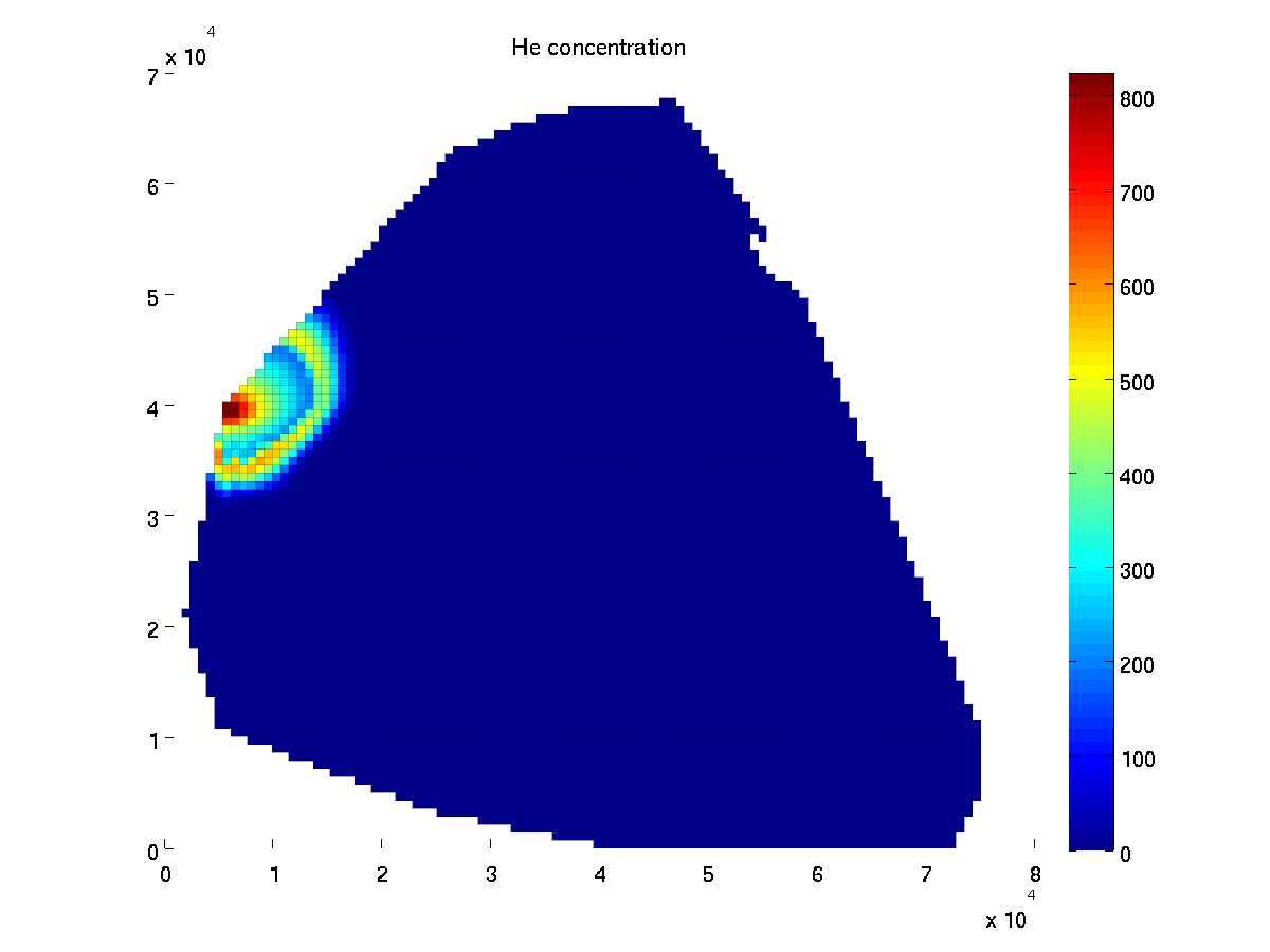
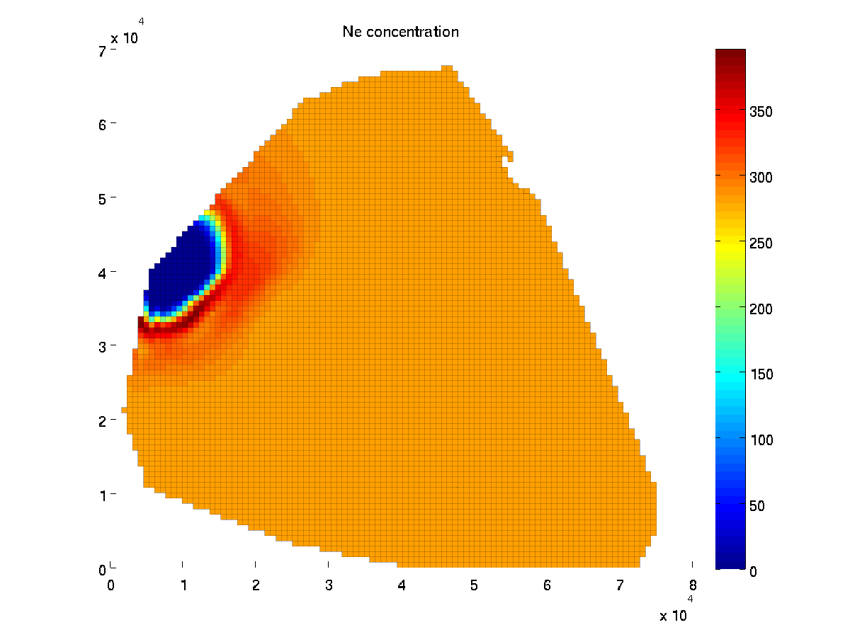
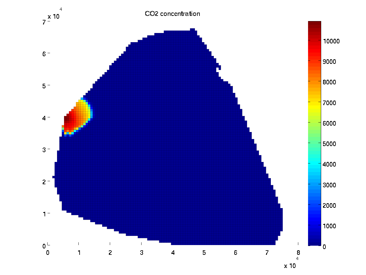
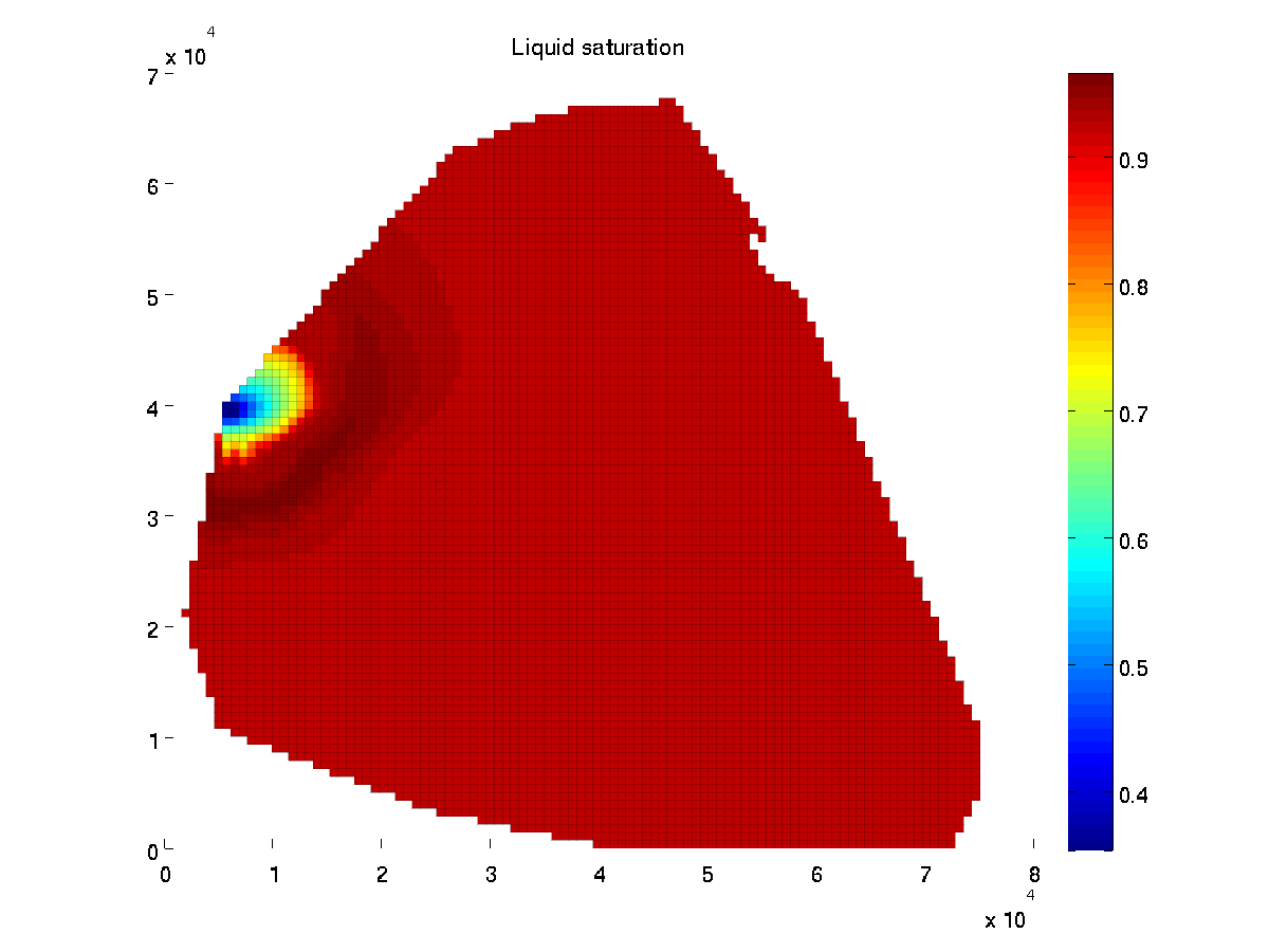
processGRDECL.m Process Eclipse grid data file.
computeGeometry.m Generate MRST grid structure.
computeTrans.m Compute the transmissibilities.
poreVolume.m Compute the cells' pore volumes.
ADI.m Class of Automatic Differentiation (AD) objects with overloading of the operators.
initVariablesADI.m Function that initiate the AD variables.
SolveEqsADI.m Assemble the Jacobians from the AD objects to form the full linear system, which is solved directly using Matlab inversion routine.
getResiduals.m Function which detects oscillations and stagnation in the Newton iterations.

Download tutorial files

tutorial-Bravo.tar.gz

Numerical results

Initially, we set the initial molar fractions of neon and water equal to 0.5% and 99.5% respectively, with no helium and carbon dioxyde. The pressure in the whole reservoir is set to the output pressure, that is, 80 bar. We inject a mixture composed of 10% Helium and 90% CO2 at a rate of 1000m^3/day. To compute the injected mole amount, we solve the flash equations assuming an injection pressure of 130 bar.

The injection is done on four cells on the western side of the reservoir and the output pressure is set on one face at the most eastern cell, see setupControls.m.

The simulation is run for 10000 days with a time step of 200 days. The following plots show the result of the simulation at end time. We observe that, as espected, the helium travels faster than the carbon dioxyde because of its lower solubility in the liquid phase.

Published October 3, 2014