Vertical-Equilibrium Models

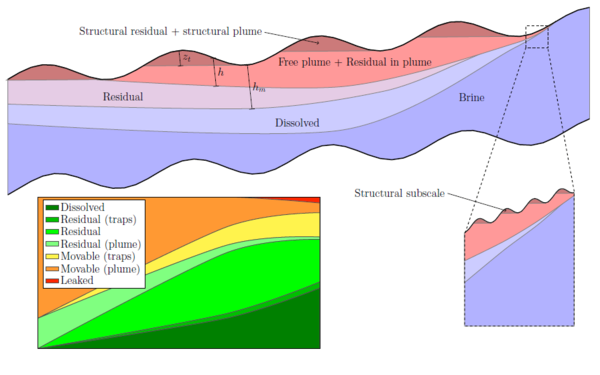
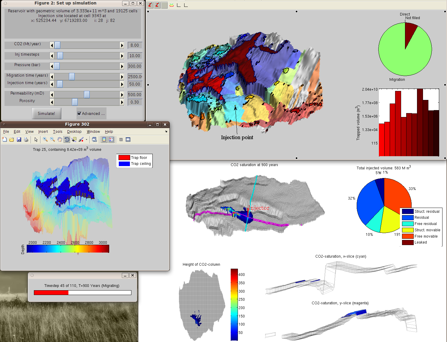
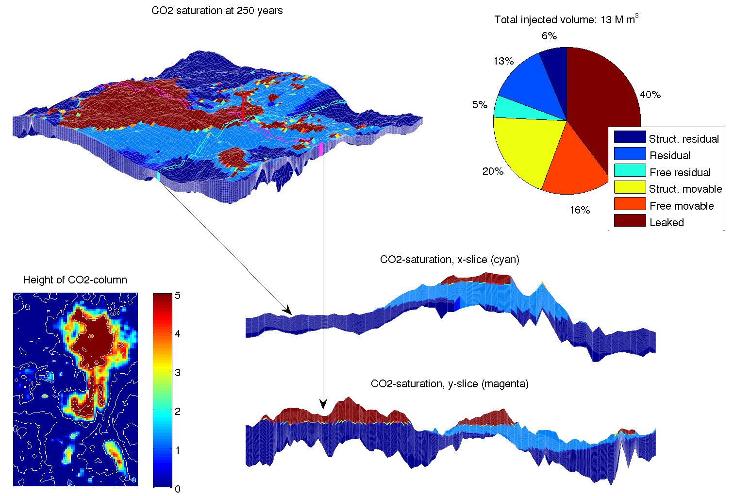
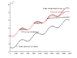
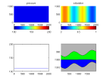
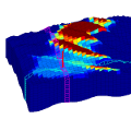
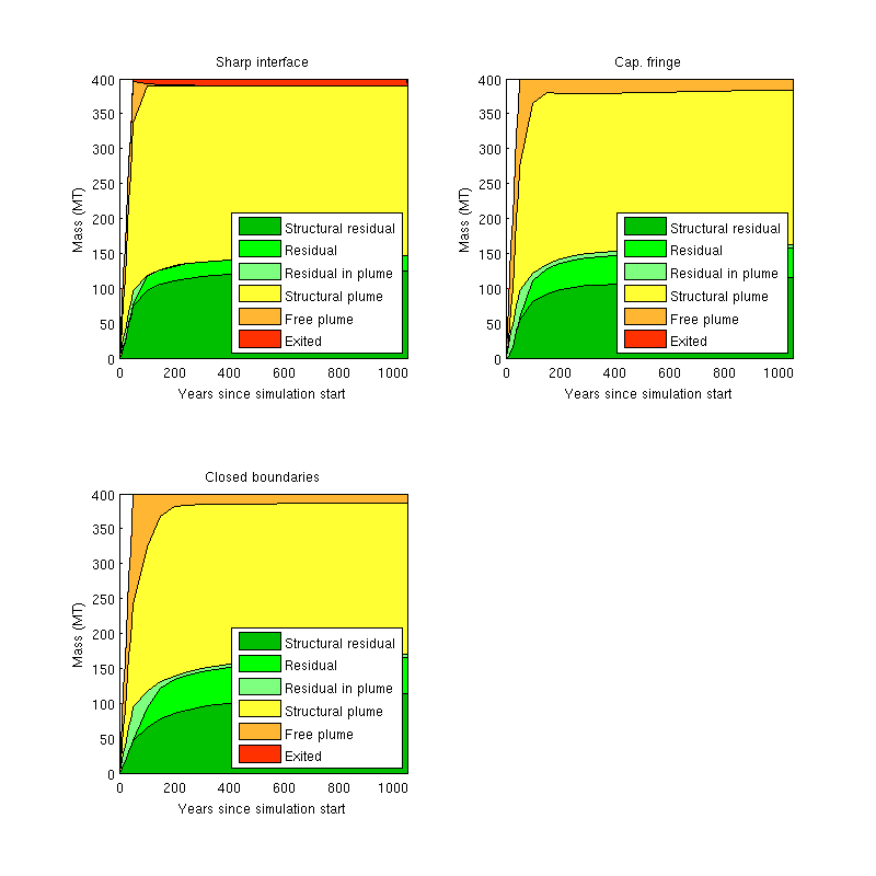
Migration of CO₂ in sloping aquifers is a truly multiscale problem with a large disparity in spatial and temporal scales. Vertical-equilibrium models offer an efficient means to accurately describe the combined large-scale and long-term effects of structural, residual, and solubility trapping. MRST-co2lab implements a wide class of vertical-equilibrium models that account for compressibility, impact of small-scale trapping, and hysteresis effects in the fine-scale capillary and relative permeability functions, using model formulations that are as close as possible to standard black-oil framework used by the petroleum industry.

Why assume vertical equilibrium?

CO₂ is very mobile and when injected into a porous rock formation, the resulting plume of supercritical fluid can travel large distances. A typical saline aquifer considered for CO₂ storage can be viewed as a thin, slightly inclined sheet that spans thousands of square kilometers. Inside this sheet, the flow of CO₂ is usually confined to thin layers underneath the sealing caprock or other low-permeable vertical barriers. This gives a large disparity in lateral and vertical scales, which in combination with differences in density between the supercritical CO₂ plume and the resident brine, means that the vertical fluid segregation will be almost instantaneous compared with the up-dip migration. The CO₂ tendency to form a relative flat fluid interface is an effect of the pressure distribution, which in turn depends strongly on the flow in the vertical direction. To avoid introducing large errors in the forecast of the updip migration, the vertical fluid distribution must therefore be represented accurately. In practice, this means using a higher grid resolution than what is computationally tractable in standard 3D simulators, and as a result, such simulations tend to be severely under-resolved unless they are conducted using large-scale systems for high-performance computing.

In a vertical equilibrium model, the primary assumption is that the flow system is in vertical equilibrium so that the vertical distribution of fluid phases can be determined from analytical expressions. One can then integrate the flow equations in the vertical direction to obtain a reduced model. This is a common approach that is used in many other branches of physics, e.g., when describing water waves, creep flow, etc. Integration in the vertical direction not only reduces the number of spatial dimensions, and hence the required number of grid cells, but will also lessens the coupling between pressure and fluid transport and improves the characteristic time constants of the problem. As a results, so-called vertical-equilibrium simulations will typically be orders of magnitude faster and consume signficantly less memory than conventional 3D simulators.

What does a VE model look like?

Using a vertical equilibrium (VE) assumption, the flow of a thin CO₂ plume in 3D can be approximated in terms of its thickness to obtain a 2D simulation model as illustrated in Figure 1. The vertical integration reduces the dimension of the model, while important information of the heterogeneities in the underlying 3D medium is preserved in an averaged sense through upscaled effective properties that depend on the particular assumption used to model the vertical fluid distribution. The integrated flow equations can be expressed on a form that resembles the standard flow equations know from the simulation of petroleum reservoirs. The only difference is that some of the new effective fluid parameters that originally only depended on saturation, now also depend on pressure.

Figure 1: Schematic illustration of how a vertical-equilibrium model is used to describe the migration and resulting trapping of CO₂ under a sloping caprock. Here, we have made the simplifying assumption that fine-scale capillary forces are negligible so that CO₂ and brine are separated by a sharp interface. The aquifer will then be filled by four different pseudo-phases, which from top to bottom are: pure CO₂, brine with residually trapped CO₂, brine with dissolved CO₂, and pure brine. If fine-scale capillary forces are included, the sharp interfaces will instead consist of a smooth transition, commony referred to as the capillary fringe.

The primary numerical formulation used in MRST-co2lab is a fully-implicit discretization. This is a pragmatic choice, motivated by the fact that if VE models are formulated in the black-oil framework, one can easily include the VE models into existing commercial and academic simulators developed for this framework and potentially develop hybrid models that combine VE and 3D models in different parts of the domain, extend the VE models with the wide range of physical effects that are described in the literature using the black-oil framework, and utilize robust and reasonably efficient numerical methods developed over the past four decades. These methods are particularly suitable for accurately computing steady states that correspond to various kinds of trapping in the long-term transient migration of CO₂. However, for simple incompressible, sharp-interface models, MRST-co2lab also offers sequential solvers.

How accurate are VE models compared with standard 3D simulation?

When studying the long-term migration of a well-formed CO₂ plume, the errors resulting from the VE assumption may be significantly smaller than the errors introduced by the overly coarse resolution needed to make the 3D simulation model computationally tractable. There are several reasons for this:

Lateral resolution: Because a VE simulator uses a 2D grid, it can typically be run with higher lateral resolution than a 3D simulation, which needs to spend the number of cells it can afford to provide a certain minimum resolution in both the lateral and the vertical direction.
Vertical resolution: Even when using a grid that is graded towards the top of the formation, a 3D simulator will typically not be able to compute the relatively sharp transition between CO₂ and brine as accurately as a VE model that uses an analytical function to this end.
Averaging of mobilities: In most cases, the fine-scale relative permeabilities k_rare nonlinear functions of saturation. Since CO₂ tends to migrate as a thin layer along the top of the domain, the fine-scale saturation s(z) can also be a nonlinear function of the height z. As a result, the vertical average value of k_r(s(z)) within a 3D grid cell may deviate significantly from k_r evaluated at the average value of s(z) within that cell. As the latter is used as an approximation in a 3D simulation, this may lead to inaccuracies that have significant effect on the resulting flow. On the other hand, in a VE model, the vertical average of k_r(s(z)) within a grid cell (a full vertical column, in this case) is obtained by vertical integration of point-wise permeability, which offers the "correct" value (as long as the vertical saturation distribution resulting from the underlying VE assumption is a good approximation).

As an illustration, see the simple comparison of VE and 3D simulations, which illustrates how a 3D simulation gradually converges to the corresponding VE simulation as the number of grid points in the vertical direction is increased.

On the other hand, traditional 3D simulation will in most cases be more suitable than using a VE approximation when simulating the fluid movement close to the injection point during injection or when simulating systems in which the migration of the CO₂ is not dominated by the topography of the caprock. One of the strenghts of MRST is that it offers both possibilities, and we even have developed example implementations that couple 3D flow equations in the near-well regions to VE models in the far-field region.

How do I perform a VE simulation?

The vertical-equilibrium simulators in MRST-co2lab can either be called from a script written for the specific case you want to investigate -- examples of such scripts are given in the tutorials below -- or you can use either of the two graphical user-interfaces that are capable of setting up a simulation.

Figures 2 and 3 show two examples of sharp-interface VE simulations. The simulations report a detailed volume inventory: residual CO₂ will not leak and can be found inside structural traps, in regions behind the tail of the plume, or within the movable plume; free CO₂ is found in traps and in the movable plume and may possibly in the future leak through holes in the caprock or reach the perimeter of the model; and finally, some CO₂ may already have exited across open boundaries. With the simplest type of sharp-interface models, a typical simulation takes from tens of seconds to a few minutes, which enables you to interactively study different injection scenarios.

Figure 2: Structural trapping and VE simulation for the Johansen formation using data from the CO₂ Storage Atlas. Once an injection point is chosen, the user can interactively change parameters such as injection rate and reservoir pressure, injection period, migration time, and homogeneous petrophysical parameters (perm and poro).

Figure 3: Vertical equilibrium simulation of the Sleipner injection, assuming a sharp interface between CO₂ and brine. The model from ieaghg.org provides injection rates for 11 years. The simulation describes 30 years of injection (using the rate of year 11 for the last 19 years), followed by 220 years of migration. See also: using VE simulation to match a benchmark model of the 9th Sleipner layer to observed plume outlines

Tutorials

The following articles gives more details about different ways of formulating VE models and performing simulations and how to construct top-surface grid that represents a 3D rock formation

	Top-surface grid We show how to make a 2D top-surface grid suitable for vertical equilibrium simulations of a small 3D grid model. The tutorial introduces and explains the basic data structure used to represent the vertically integrated model in the VE solvers.			Comparison of VE formulations There are several ways to formulate a vertical equilibrium model. This example demonstrates and compares two approaches: One uses the height h of the CO₂column as the primary variable, the other the fractional height S=h/H.

	VE in a regular black-oil solver In this example we show how to set up a standard format black-oil model that can be used to simulate a VE model. For the actual simulation, we use the fully-implicit solver in MRST from the 'ad-fi' module, which is based on automatic differentiation.			Small sloping aquifer We make a model of a syntetic sloping aquifer and demonstrate the use of the vertical equilibrium module for simulating injection and migration of CO₂ on this model.

	Fully-implicit VE simulation using class-based black-oil programming framework Since the MRST2015a, a new, class-based framework for setting up fully-implicit simulations in a simple way has been introduced. Here, we use the framework to setup and run multiple simulations of an injection scenario, using different assumptions on boundary conditions and capillary pressure.			Multilayered system with caprock leakage This example shows a conceptual model of a multilayered system where there is leakage through the caprock that delineates each layer. The system is simulated using a standard fully-implicit simulator with a fluid model that mimics a vertical equilibrium formulation.