Contents

VE simulation with capillary fringe using black-oil solver

In this example, we will run three separate simulations of injection and migration of CO₂ into the Gassum formation. We will look at the impact of boundary conditions on pressure buildup, as well as the effect on the plume shape of including a capillary fringe. The present demonstration employs the new, class-based framework for setting up simulations. This framework was introduced into MRST-co2lab in the 2015a release. Previous to that release, fully-implicit simulations were carried out using the approach demonstrated in this tutorial.

% The following line ensures we have the necessary modules loaded
moduleCheck co2lab ad-core libgeometry

% Ensure gravity is in effect
gravity on

Setting initial parameters

We start by setting some initial parameters that will be used further down. We use the struct 'opt' to keep track of all simulation parameters.

opt.sf_temp = 7;                       % temperature at seafloor (degrees centigrade)
opt.sf_depth = 100;                    % seafloor depth in meters
opt.tgrad = 35;                        % thermal gradient, degrees centigrade / km depth
opt.wellpos = [7.55e5, 6.39e6];        % injection site coordinates
opt.annual_injection = 8 * mega * 1e3; % inject eight megatons per year
opt.res_sat = [0.11, 0.21];            % water and CO2 residual saturation
opt.injection_time = 50 * year;        % total injection time
opt.migration_time = 1000 * year;      % total migration time
opt.injection_steps = 10;              % simulation timesteps during injection phase
opt.migration_steps = 20;              % simulation timesteps during migration phase

Load simulation grid and rock structure

As our simulation domain, we will use the "Gassum" formation. For convenience we downsample the grid a bit, so that simulation runtimes will be shorter.

coarsening_level = 3; % grid downsampling factor (1 = no downsampling)
[Gt, rock2D] = getFormationTopGrid('Gassumfm', coarsening_level);

Show simulation grid

We plot the simulation grid for inspection.

plotCellData(Gt, Gt.cells.z, 'edgealpha', 0.4); view(56, 76);
set(gcf, 'position', [10 10 800 600]);
axis tight; colorbar;

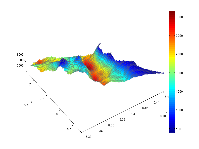
Plotting injection well on formation grid

We notice that the formation has large variation in depth, from less than 500 meters to more than 3500 meters below sea level. There are also several large traps. Our intention is to inject CO₂ close to the lowermost point, but within the spill region of a large trap. One such position is given by our choice of well position specified above. We setup our well and plot it on the simulation grid to visualize this.

% Here we identify the cell of the simulation grid that is closest to the chosen
% well position, and designating this as the well cell.
dist2 = bsxfun(@minus, Gt.cells.centroids, opt.wellpos);
dist2 = sum(dist2.^2,2); % squared distance cell centre to inj. point
[~, wcell_ix] = min(dist2); % index of cell closest to inj. point

% Here we set up the well.  We need the fluid object to compute the exact
% volumetric rate, so we use a dummy rate for the time being, and will set it
% correctly once the fluid has been specified further down.

W = addWell([], Gt, rock2D, wcell_ix , ...
            'type'   , 'rate'        , ...
            'val'    , 0.1           , ... % dummy val
            'comp_i' , [0 1]);

% Let us plot the well on the grid to check that we got the position right.
plotCellData(Gt, Gt.cells.z, 'edgealpha', 0.4);
plotWell(Gt.parent, W, 'color', 'k');
set(gcf, 'position', [10, 10, 800, 600]); view(76, 66);

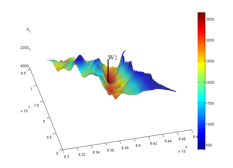
We see on the figure that the well has been placed towards the bottom, and located in a place where gravity-driven flow will lead CO₂ up to the large pockets on the immediate left on the figure.

Setup fluid objects (with and without capillary fringe)

In addition to the simulation grid and the rock object, a simulation needs a fluid object (which describes fluid properties for both phases, like density, viscosity, relative permeabilities and capillary pressure), an initial state, boundary conditions and an injection schedule. We will proceed to construct these below. We start with the fluid object. A fully-featured fluid object can be constructed with the makeVEFluid function. Below, we define two different fluid objects. The first one represents a fluid system with a sharp interface between CO₂ and brine, the second represents a fluid system with a capillary fringe between the two phases. Further down, we will compare simulation results using these different fluid systems.

% Aquifer temperature field (necessary to compute local CO₂ density).  The
% temperature field depends on the seafloor temperature, the depth of the
% caprock, and the thermal gradient.
T = 273.15 + opt.sf_temp + (Gt.cells.z - opt.sf_depth) / 1e3 * opt.tgrad;

% Sharp-interface type fluid
fluid_si = makeVEFluid(Gt, rock2D, 'sharp interface' , ...
                       'fixedT'   , T                , ...
                       'residual' , opt.res_sat);

% Fluid with linear capillary fringe
fluid_cf = makeVEFluid(Gt, rock2D, 'P-scaled table'  , ...
                       'fixedT'   , T                , ...
                       'residual' , opt.res_sat);

% We can now set the correct injection rate for the well.  The injection rate
% should be volumetric, so we divide the desired mass by the by the reference
% CO₂ density, as provided by the fluid object.
W.val = opt.annual_injection / year / fluid_si.rhoGS;

Setup initial state in the aquifer

We now specify the initial conditions in the aquifer prior to injection. For each cell in the grid, we need to define the pressure and the fluid saturation. In addition, we keep track of the historical maximum CO₂ concentration for each cell, which is zero at simulation start.

% We use water density at reference conditions ('rhoWS') to compute
% (approximate) hydrostatic aquifer pressure.
initState.pressure = Gt.cells.z * norm(gravity) * fluid_si.rhoWS;
initState.s = repmat([1 0], Gt.cells.num, 1); % [initial water and CO2 saturations]
initState.sGmax = initState.s(:,2); % historically maximum CO2 saturation

Setup boundary conditions, injection well and schedule

We now define the aquifer boundary conditions and the injection schedule. We will prepare two different sets of boundary conditions for the aquifer, fully closed and fully open boundaries, so that we can compare the outcome further down. In addition to boundary conditions, an injection schedule specifies the timestep lengths and the state of the injection well at each timestep. We use it to define an injection period, where our well will be injecting CO₂, and a migration period where our well will be inactive. We thus have to prepare two injection schedules, one for each set of boundary conditions.

% 'W_off' will represent our well during the migration phase.  It is identical
% to our well object 'W', except that the well rate has been set to zero.
W_off = W;
W_off.val = 0; % During migration, the rate through the well is zero.

% The line below identifies all the boundary faces of our simulation grid.
bfaces = find(any(Gt.faces.neighbors==0, 2));

% We specify a set of boundary conditions here all boundary faces are
% 'open' (permit flow), and we specify the pressure value on these faces as
% being hydrostatic.
open_bc = addBC([], bfaces, ...
                'pressure', Gt.faces.z(bfaces) * fluid_si.rhoWS * norm(gravity), ...
                'sat', [1 0]);

% Compute steplengths
istep = diff(linspace(0, opt.injection_time, opt.injection_steps + 1));
mstep = diff(linspace(0, opt.migration_time, opt.migration_steps + 1));

% Define schedule with closed boundaries (the absence of boundary conditions
% is equivalent to closed boundaries)
schedule_cb.control = [struct('W', W, 'bc', []), ...   % well and bc during injection
                       struct('W', W_off, 'bc', [])];  % well and bc during migration
schedule_cb.step    = struct('control', [1 * ones(size(istep)), ...
                                         2 * ones(size(mstep))], ...
                             'val', [istep, mstep]);

% Define schedule with open boundaries.  The schedule object is equal to the
% one for closed boundaries, except that we add on the open boundary
% contitions we just prepared above.
schedule_ob = schedule_cb;
schedule_ob.control(1).bc = open_bc; % open boundaries during injection
schedule_ob.control(2).bc = open_bc; % open boundaries during migration

Setup simulation models

We now construct the full simulation model object, which includes grid, rock and fluids. In fact, we construct two such objects, one for the sharp interface case, another for the case with a capillary fringe.

model_si = CO2VEBlackOilTypeModel(Gt, rock2D, fluid_si);
model_cf = CO2VEBlackOilTypeModel(Gt, rock2D, fluid_cf);

We now run our simulations. We consider the following cases:

% Run simulation with open boundaries and sharp interface
[wellSols_si, states_si] = simulateScheduleAD(initState, model_si, schedule_ob);

% Run simulation with open boundaries and capillary fringe
[wellSols_cf, states_cf] = simulateScheduleAD(initState, model_cf, schedule_ob);

% Run simulation with closed boundaries
[wellSols_cb, states_cb] = simulateScheduleAD(initState, model_si, schedule_cb);

Comparing results

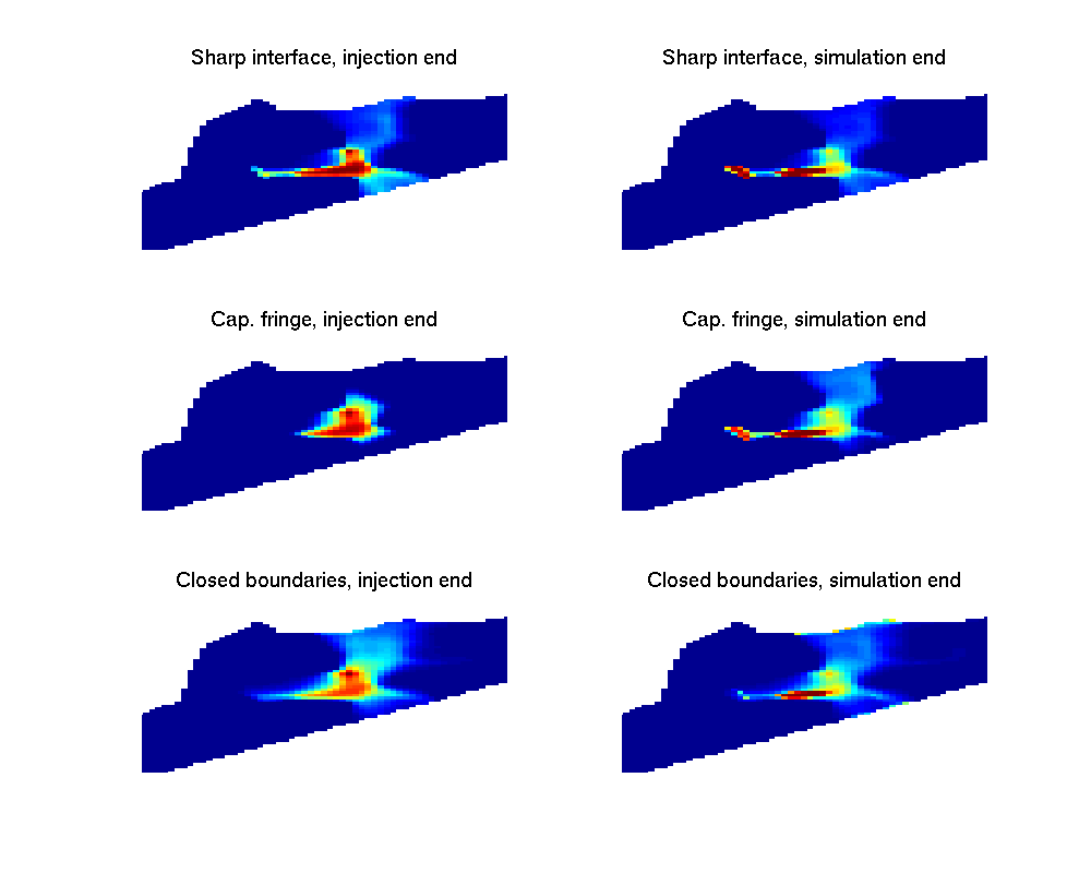
We now want to compare the outcomes from our three simulations. We will inspect the state of the aquifer at the end of injection and migration periods. We start out comparing saturations. A naive plot gives us the following diagrams:

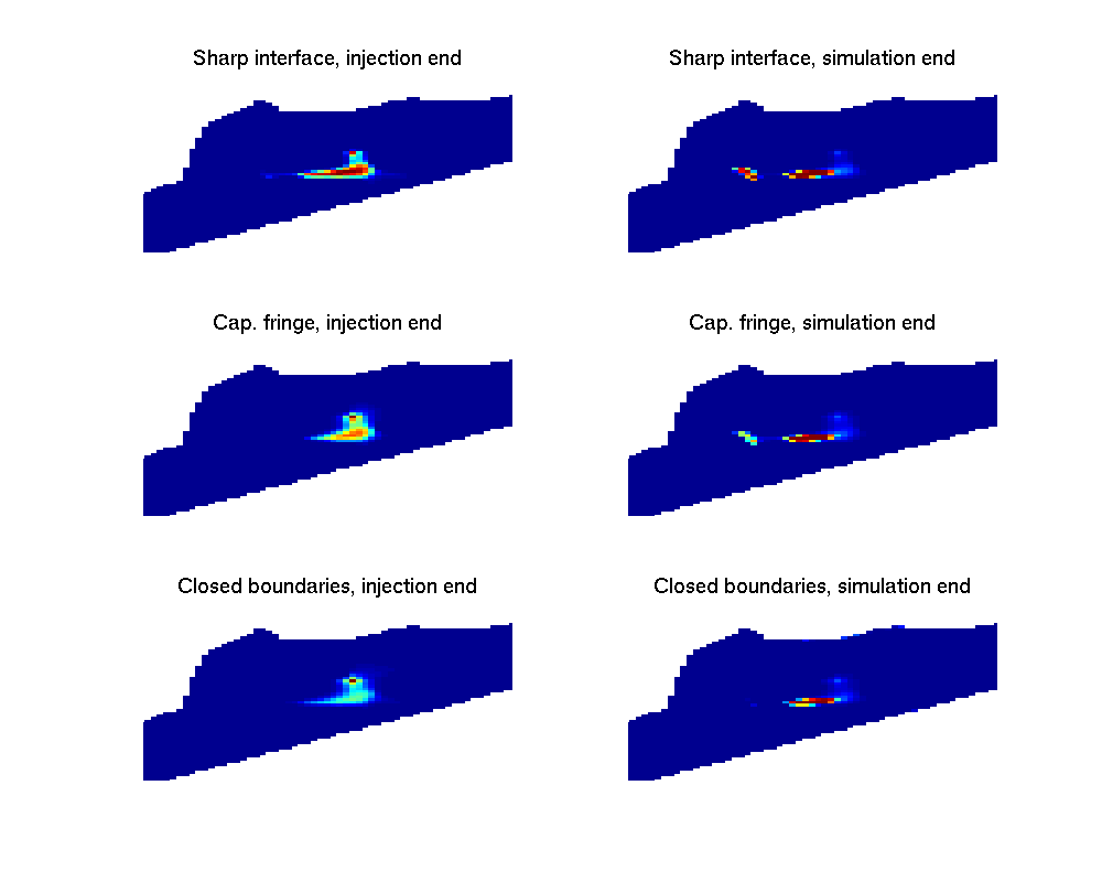
On these plots, we can notice some differences, but it is not easy to compare since regions with low nonzero CO₂ saturations are hard to distinguish from regions with no CO₂ at all. One way of emphasizing regions with low saturations is to visualize the saturation raised to a fractional power (square root, etc.) We here produce the same plot as above, but raise all saturations to the power of 1/4 (i.e. taking the square root of the square root).

Comparing overpressure at end of injection and end of migration

We now proceed to compare overpressure (difference between actual and initial pressure) for the three simulation cases. We expect the boundary conditions to have a large impact on the overpressure.

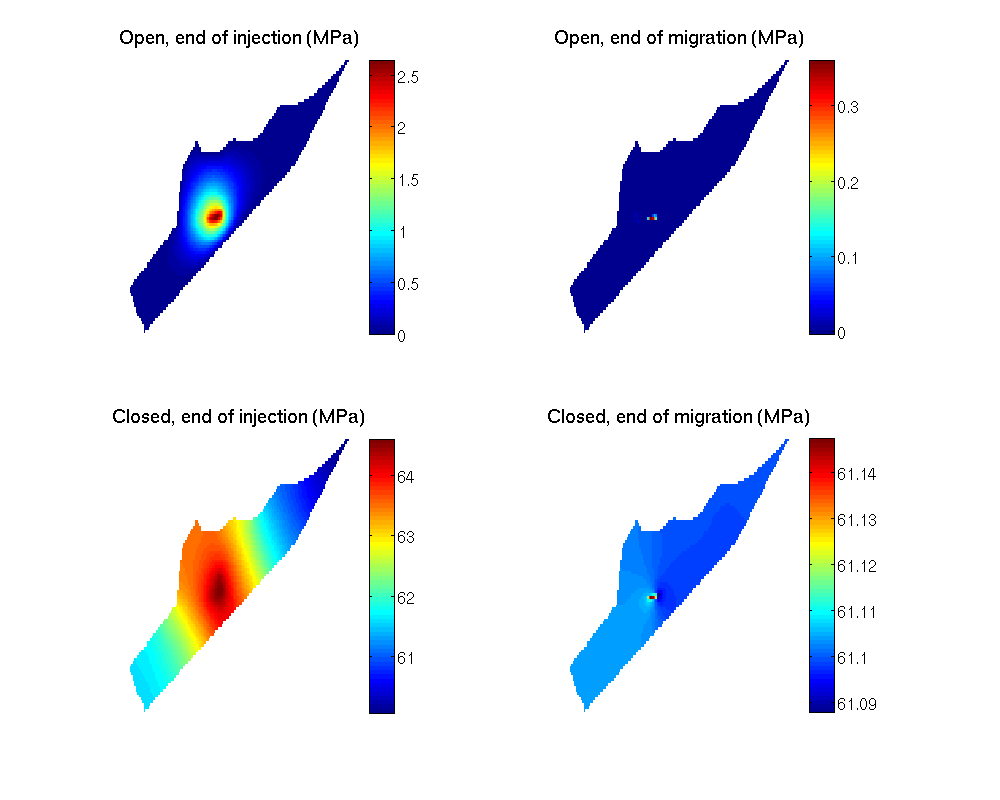
As can be seen from the plot, there are significant quantitive and qualitative differences between the result using different boundary conditions. The overpressure never reaches more than 2.5 MPa in the open boundary cases, whereas it rises to more than 64 MPa for closed boundaries. Moreover, whereas overpressure basically drops to zero during the migration period in the open boundary case, it stabilizes at about 61 MPa everywhere in the aquifer when boundaries are closed.

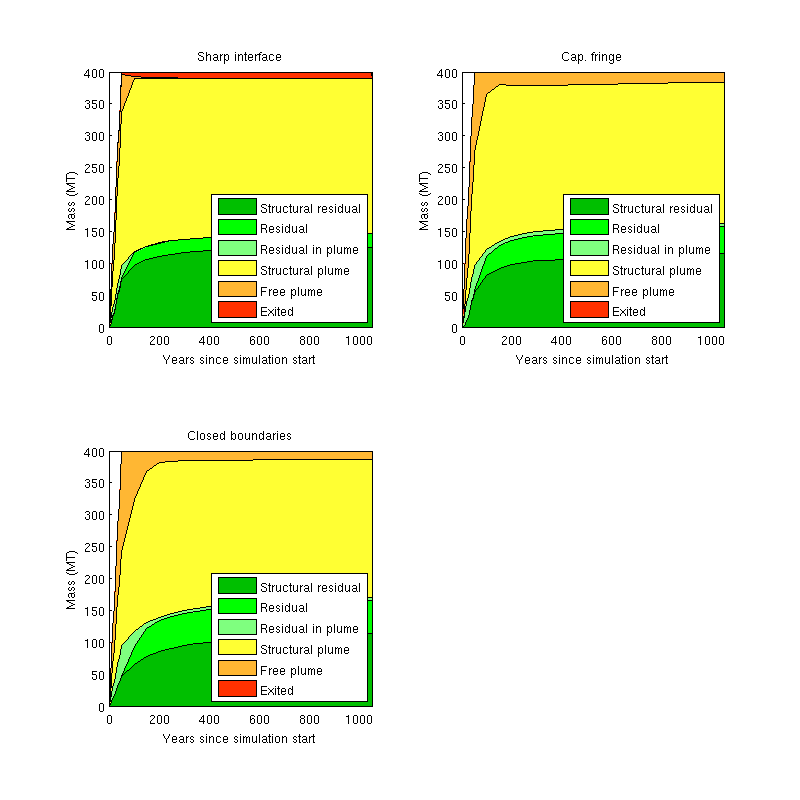
Tracking CO₂ trapping states: comparing inventory plots

Finally, we compare the trapping states over time for the three simulations. We do this by constructing and comparing inventory plots. Currently, the routine for doing so (plotTrappingDistribution) require the simulation results to be packaged and presented in a certain way, as done by the makeReports function. We thus use this function to prepare the necessary reports before producing our plots.

In order to compute the amount of CO₂ in structural traps, the makeReports function needs to know the location of the structural traps. This information is generated as part of the trapping analysis, which is carried out by the trapAnalysis function.

ts = trapAnalysis(Gt, false);

% We now generate the reports needed by |plotTrappingDistribution|.
report_si = makeReports(Gt, [{initState}; states_si], rock2D, fluid_si, ...
                        schedule_ob, opt.res_sat, ts, []);
report_cf = makeReports(Gt, [{initState}; states_cf], rock2D, fluid_cf, ...
                        schedule_ob, opt.res_sat, ts, []);
report_cb = makeReports(Gt, [{initState}; states_cb], rock2D, fluid_si, ...
                        schedule_cb, opt.res_sat, ts, []);

% We finally generate and plot the inventory plots for our three simulations
h = figure;
subplot(2,2,1); ax = get(h, 'currentaxes');
plotTrappingDistribution(ax, report_si, 'legend_location' ,'southeast'); axis tight;
title('Sharp interface');
subplot(2,2,2); ax = get(h, 'currentaxes');
plotTrappingDistribution(ax, report_cf, 'legend_location' ,'southeast'); axis tight;
title('Cap. fringe');
subplot(2,2,3); ax = get(h, 'currentaxes');
plotTrappingDistribution(ax, report_cb, 'legend_location', 'southeast'); axis tight;
title('Closed boundaries');
set(gcf, 'position', [10 10 800 800]);