Please note that this example requires a Black-Oil solver that was included since the 2013a release.  This solver has been superceded by a class-based framework for setting up and running fully-implicit simulations. See here for an example on how to use the new, class-based framework with MRST-co2lab.

• Parameters for the simulation
• Create input deck and construct grid
• Initialize data structures
• Run the schedule setup in the file
• Plot results

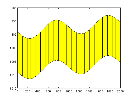
VE simulation in a standard black-oil solver

In this example we show how to set up a standard format black-oil model that can be used to simulate a VE model. For the actual simulation, we use the fully-implicit solver in MRST from the 'ad-fi' module, which is based on automatic differentiation.

try
   require deckformat ad-fi
catch %#ok<CTCH>
   mrstModule add deckformat ad-fi
end

Parameters for the simulation

gravity on
[nx,ny,nz] = deal(40, 1, 1);     % Cells in Cartsian grid
[Lx,Ly,H]  = deal(2000,1000,15); % Physical dimensions of reservoir
total_time = 5*year;             % Total simulation time
nsteps     = 10;                 % Number of time steps in simulation
dt         = total_time/nsteps;  % Time step length
perm       = 100;                % Permeability in milli darcies
phi        = 0.1;                % Porosity
depth      = 1000;               % Initial depth
ipress     = 200;                % Initial pressure

Create input deck and construct grid

Create an input deck that can be used together with the fully-implicit solver from the 'ad-fi' module. Since the grid is constructed as part of setting up the input deck, we obtain it directly.

[deck, G] = sinusDeckAdi([nx ny nz], [Lx Ly H], nsteps, dt, ...
                         -.1*pi/180, depth, phi, perm, ...
                         (H*phi*Lx*Ly)*0.2*day/year, ipress);

% Alternatively, we could read deck from file and construct the grid
% deck = readEclipseDeck( ...
%    fullfile(VEROOTDIR,'data','decks','sinusDeckAdi.DATA');
% G = initEclipseGrid(deck);

figure, plotGrid(G),view([0 -1 0]), box on

Initialize data structures

First, we convert the input deck to SI units, which is the unit system used by MRST. Second, we initialize the rock parameters from the deck; the resulting data structure may have to be post-processed to remove inactive cells. Then we set up the fluid object and tell the ad-fi solver that that we are working with an oil-water system.

deck  = convertDeckUnits(deck);
rock  = initEclipseRock(deck);
rock  = compressRock(rock, G.cells.indexMap);
fluid = initDeckADIFluid(deck);
systemOW  = initADISystem({'Oil', 'Water'}, G, rock, fluid);

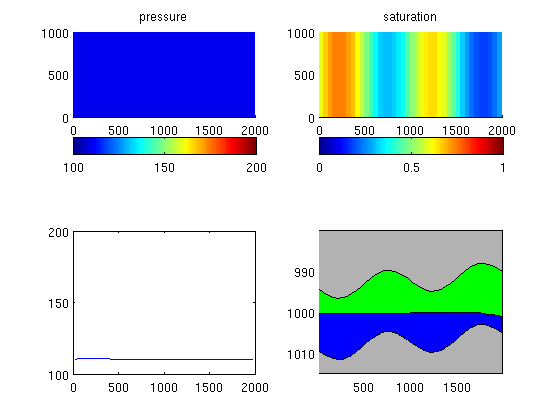
Run the schedule setup in the file

Before we can run the schedule, we make sure that we have an initial hydrostatic pressure distribution. Then we pick the schedule from the input deck and start the simulator.

x0 = initEclipseState(G, deck, initEclipseFluid(deck));
z  = G.cells.centroids(:,3);
x0.pressure = ipress*barsa +(z(:)-z(end))*norm(gravity)*deck.PROPS.DENSITY(2);

[wellSols, states] = runScheduleADI(x0, G, rock, systemOW, deck.SCHEDULE);

Warning: Non-linear solver did not converge, stopped by max iterations... 
Step    1 of   20 (Used  25 iterations)
Step    2 of   20 (Used  10 iterations)
Step    3 of   20 (Used   4 iterations)
Step    4 of   20 (Used   4 iterations)
Step    5 of   20 (Used   4 iterations)
Step    6 of   20 (Used   4 iterations)
Step    7 of   20 (Used   3 iterations)
Step    8 of   20 (Used   3 iterations)
Step    9 of   20 (Used   3 iterations)
Step   10 of   20 (Used   3 iterations)
Warning: Injector 'I01' shut on input.  Ignored.
 
Warning: Number of wells has changed, wellsol field should be updated based on well-name matching 
Step   11 of   20 (Used   7 iterations)
Step   12 of   20 (Used   4 iterations)
Step   13 of   20 (Used   3 iterations)
Step   14 of   20 (Used   3 iterations)
Step   15 of   20 (Used   3 iterations)
Step   16 of   20 (Used   3 iterations)
Step   17 of   20 (Used   3 iterations)
Step   18 of   20 (Used   3 iterations)
Step   19 of   20 (Used   3 iterations)
Step   20 of   20 (Used   3 iterations)

Plot results

%figure
Gt = topSurfaceGrid(G);
xc = Gt.cells.centroids(:,1);
zt = Gt.cells.z;
zb = zt + Gt.cells.H;
for nn=1:numel(states)
    clf
    state=states{nn};

    subplot(2,2,1),cla
    title('pressure')
    plotCellData(G,state.pressure/barsa);colorbar('horiz'), caxis([100 200])

    subplot(2,2,2),cla
    title('saturation')
    plotCellData(G,state.s(:,1));colorbar('horiz'), caxis([0 1])

    % plot as VE
    subplot(2,2,3),cla
    plot(xc,state.pressure/barsa); set(gca,'YLim',[100 200]);

    subplot(2,2,4),cla,hold on
    patch(xc([1 1:end end]), [zt(end)-10; zt; zt(end)-10],.7*[1 1 1]);
    patch(xc([1 1:end end]), [zb(end)+10; zb; zb(end)+10],.7*[1 1 1]);
    patch(xc([1:end end:-1:1]), ...
      [zt + Gt.cells.H.*state.s(:,2); zt(end:-1:1)], 'g')
    patch(xc([1:end end:-1:1]), ...
      [zt + Gt.cells.H.*state.s(:,2); zb(end:-1:1)], 'b')
    set(gca,'YDir','reverse'), axis tight

    drawnow;
    pause(0.01)
end