MRSTlogo_web_banner_light_thinner_Epi.png

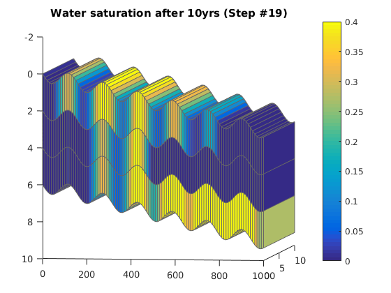
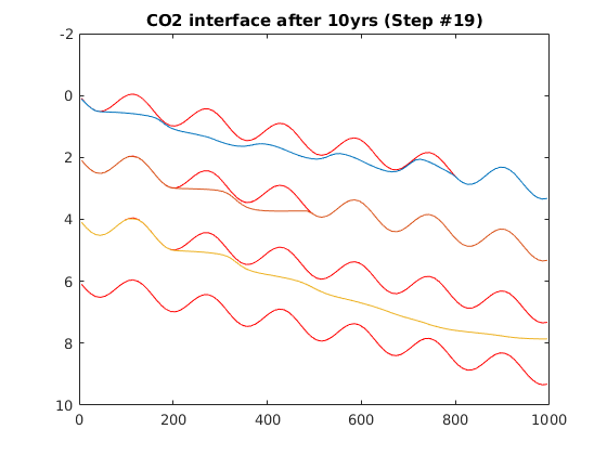
Simulating Leakage in a Multilayered System

Contents

VE simulation of CO2 injection in a multilayered system

In the example, we look at a mockup system with multiple sandbodies separated by inclined, undulating caprock layers that contain leakage points. The caprock layers are modelled by setting the vertical transmissibilities to be zero, whereas the leakage points are modelled using wells with a total rate set to zero. With this setup, we can have inflow in one perforation and outflow in another. CO2 is injected in the deepest part of the lower layer. To simulate the injection process, we use a fully-implicit, two-phase, black-oil simulator from MRST.

mrstModule add ad-core ad-blackoil ad-props mrst-gui

Aquifer geometry, petrophysical data, and boundary conditions

Simple geometry: three layers of sand having a 0.3% inclination and an undulating top surface.

[nz,dz]=deal(3,2);
gravity on;
G=cartGrid([100,1,nz],[1000,10,nz*dz]);
theta=0.003;
G.nodes.coords(:,3) = G.nodes.coords(:,3) + ...
    (G.nodes.coords(:,1)*theta+sin(G.nodes.coords(:,1)*0.04)*dz*0.2);
G=computeGeometry(G);
rock.perm = 1000*milli*darcy*ones(G.cells.num,1);
rock.poro = 0.1*ones(G.cells.num,1);
bc = pside([], G, 'Right', 100*barsa,1,1,'sat',[1 0]);
figure, h=plotGrid(G); view([0 -1 0]), box on

Fluid model

Instead of using one of the VE fluid models from the co2lab module, we simply use a model with linear relative permeabilities, which is is essentially what we would get by performing a vertical integration. However, we modify the capillary pressure so that it corresponds to the second-order term that comes out of the vertical integration

rho_b = 1000 * kilogram / meter^3;
mu_b  = 2.535e-4 * Pascal * second;
rho_c = 696 * kilogram / meter^3;
mu_c  = 3.950e-5 * Pascal * second;
fluid = initSimpleADIFluid('mu', [mu_b mu_c 1], 'rho', ...
                           [rho_b rho_c 1], 'n', [1 1 1]);
H = repmat(dz,G.cells.num,1);
fluid.pcOW = @(s)...
    -norm(gravity)*(rho_b-rho_c)*(s.*H+0*G.cells.centroids(:,3));

Transmissibility

Remove transmissibilities on top and bottom to model the caprocks that delimit the individual layers

grdecl.MULTZ = zeros(G.cartDims);
T = computeTrans(G, rock);%,'grdecl',grdecl);
T = 1./accumarray(G.cells.faces(:,1),1./T,[G.faces.num,1]);
pv = poreVolume(G,rock);
tpv = sum(pv);
topb = accumarray(G.cells.faces(:,1), ...
    any(bsxfun(@eq,G.cells.faces(:,2),[5,6]),2),[G.faces.num,1]);
topb = topb>0;
T(topb)=0;
set(h,'FaceAlpha',.4); plotFaces(G,topb,'FaceColor','r'); view(8,3);

Model

The model is a special case of a two-phase oil-water model

model = TwoPhaseOilWaterModel(G, rock, fluid); %'trans',T,'porv',pv);
model.operators = setupOperatorsTPFA(G, [], 'trans',T,'porv',pv);

Set initial state

We assume that some CO2 has already been injected into the formation to fill the deepest part of layer 3.

[i,j,k] = ind2sub(G.cartDims,G.cells.indexMap);
cells = find(k==G.cartDims(3));
s_co2 = (-((G.cells.centroids(:,1)-100*k*3)/300).^2+0.8).*(k==3);
s_co2(s_co2<0,:) = 0;
s = [1-s_co2,s_co2];
state = initResSol(G, 100*barsa, s);
delete(h);
plotCellData(G, state.s(:, 1),'FaceAlpha',.8)
title('Initial water saturation')
colorbar

Set wells

We have one injection well that is completed in the lower sand body, in which we will inject CO2. The other two wells are used to model leakage pathways and are hence assigned to have zero total rate. This will issue a warning that can be ignored.

end_time=10*year;
W3d = verticalWell([], G, rock,  floor(G.cartDims(1)*3/4), 1,3:3,     ...
                     'Type', 'rate', 'Val', tpv*0.1./end_time, ...
                     'Radius', 0.125, 'Name', 'I1');

W3d = verticalWell(W3d, G, rock,  floor(G.cartDims(1)*3/7), 1,2:G.cartDims(3),     ...
                     'Type', 'rate', 'Val', 0.0, ...
                     'Radius', 1.125, 'Name', 'C1');
W3d = verticalWell(W3d, G, rock,  floor(G.cartDims(1)*4/14), 1,1:G.cartDims(3),     ...
                     'Type', 'rate', 'Val', 0.0, ...
                     'Radius', 1.125, 'Name', 'C2');
for i=1:numel(W3d)
   W3d(i).compi=[0,1];
end
plotWell(G,W3d)
Warning: Given value is zero, prod or inj ??? 

Perform simulation

We first make a simple schedule consisting of equally-spaced time steps and then run the resulting simulation using a fully-implicit simulator

dt = diff(linspace(0,end_time,20))';
schedule = simpleSchedule(dt, 'bc', bc,'W',W3d);

[wellSols, states] = simulateScheduleAD(state, model, schedule, 'Verbose', true);
*****************************************************************
********** Starting simulation:    19 steps,  3650 days *********
*****************************************************************
Solving timestep 01/19:  -> 192 Days, 2 Hours, 1894 Seconds, 736 Milliseconds
Completed 15 iterations in 0.69 seconds (0.05s per iteration)
:
:
:
Solving timestep 19/19: 9 Years, 172 Days, 21 Hours, 1705 Seconds, 263 Milliseconds -> 10 Years
Completed 3 iterations in 0.16 seconds (0.05s per iteration)

*** Simulation complete. Solved 19 control steps in 4 Seconds, 975 Milliseconds ***


Play a movie of the results, shown as 3D grid

h = figure();
for i = 1:numel(states)
    figure(h); clf;

    % Plotting
    plotCellData(G, states{i}.s(:, 2))
    title(['Water saturation after ', num2str(sum(dt(1:i))/year), ...
        'yrs (Step #', num2str(i), ')']);

    % Make axis equal to show column structure
    %axis equal tight off
    view(8, 4)
    colorbar
    caxis([0, 0.4])

    pause(0.5)
end

Play a movie of the interface between CO2 and brine

x2d=reshape(G.cells.centroids(:,1),G.cartDims(1),G.cartDims(3));
z2d=reshape(G.cells.centroids(:,3),G.cartDims(1),G.cartDims(3));
for j=0:numel(states);
    if(j==0)
        sol3d=state;
    else
        sol3d=states{j};
    end
    sat2d=reshape(sol3d.s(:,2),G.cartDims(1),G.cartDims(3));
    figure(33),clf
    for i=1:G.cartDims(3)
        plot(x2d(:,i),z2d(:,i)-dz/2,'r');hold on
        plot(x2d(:,i),z2d(:,i)+dz/2,'r');hold on
        plot(x2d(:,i),sat2d(:,i)*dz+z2d(:,i)-dz/2)
        title(['CO2 interface after ', num2str(sum(dt(1:j))/year), ...
            'yrs (Step #', num2str(j), ')']);
        set(gca,'Ydir','reverse')
        hold on
    end
    pause(0.1)
    hold off
end


Published February 3, 2016