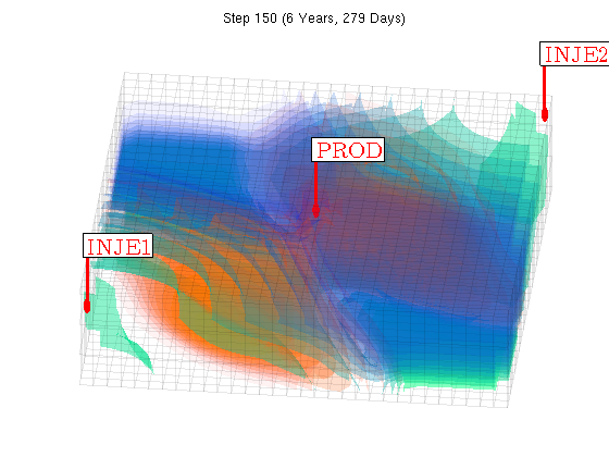
In this tutorial, we set up a two phases flow simulator with polymer. The polymer model which is used is similar to the one implemented in Eclipse model, see tutorial polymer note, and Eclipse input format can be used to set the parameters of the polymer model.

Here, we present two solvers: runPolymer.m and runLabPolymer.m. The source files for this tutorial can be found here: tutorial-polymer.tar.gz.

The first solver, runPolymer.m, is a polymer solver which is already integrated in MRST. It uses the object oriented framework developed for reservoir models. As the code shows, it is easy to set up. Two test cases are run. The first one with polymer injection with maximum polymer concentration at the injectors. The complete schedule as well as the fluid properties can be found in POLYMER.DATA. The second one without polymer. Below we plot the result for the last time step with polymer. The isolines for water saturation (in green-blue colors) and polymer (in orange colors) are shown. See more plot results in runPolymer.m.

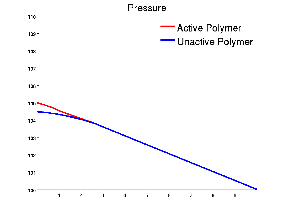
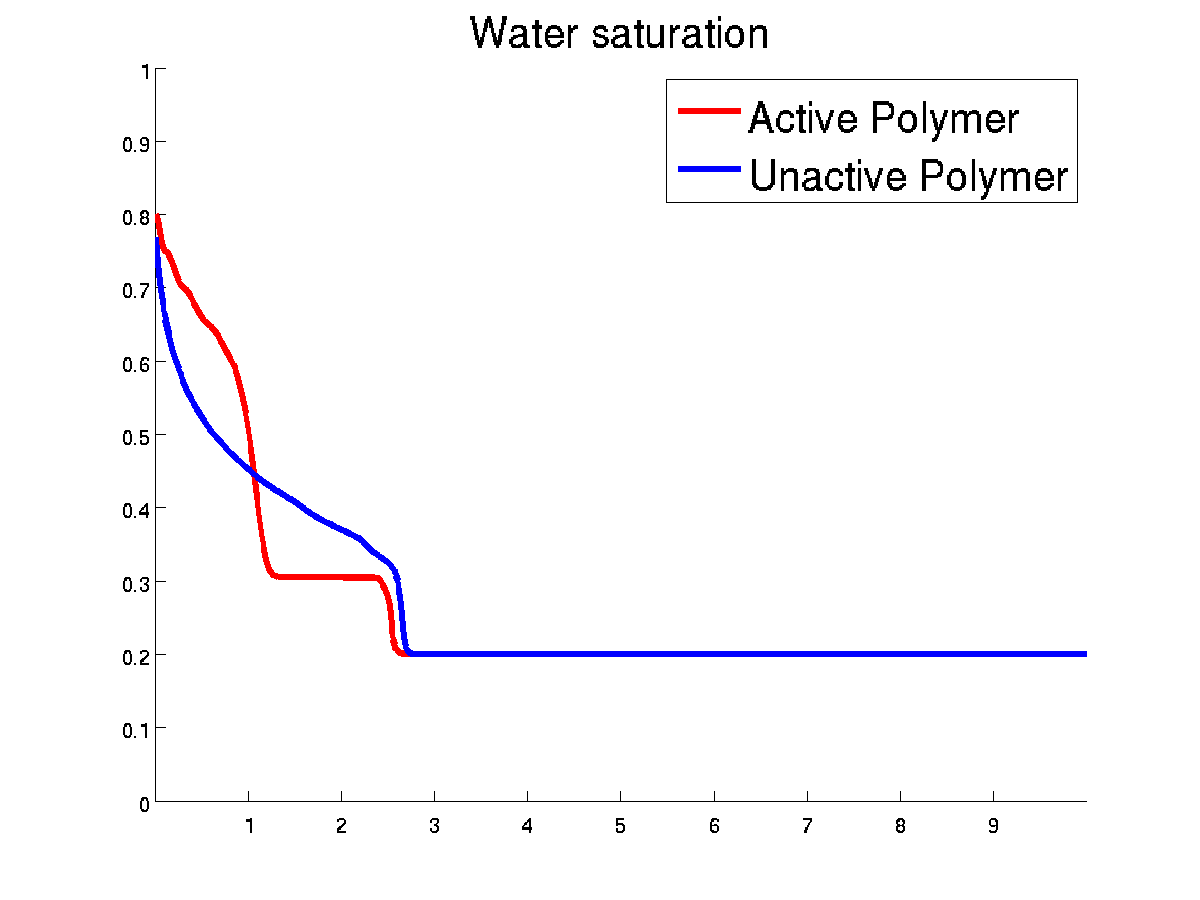
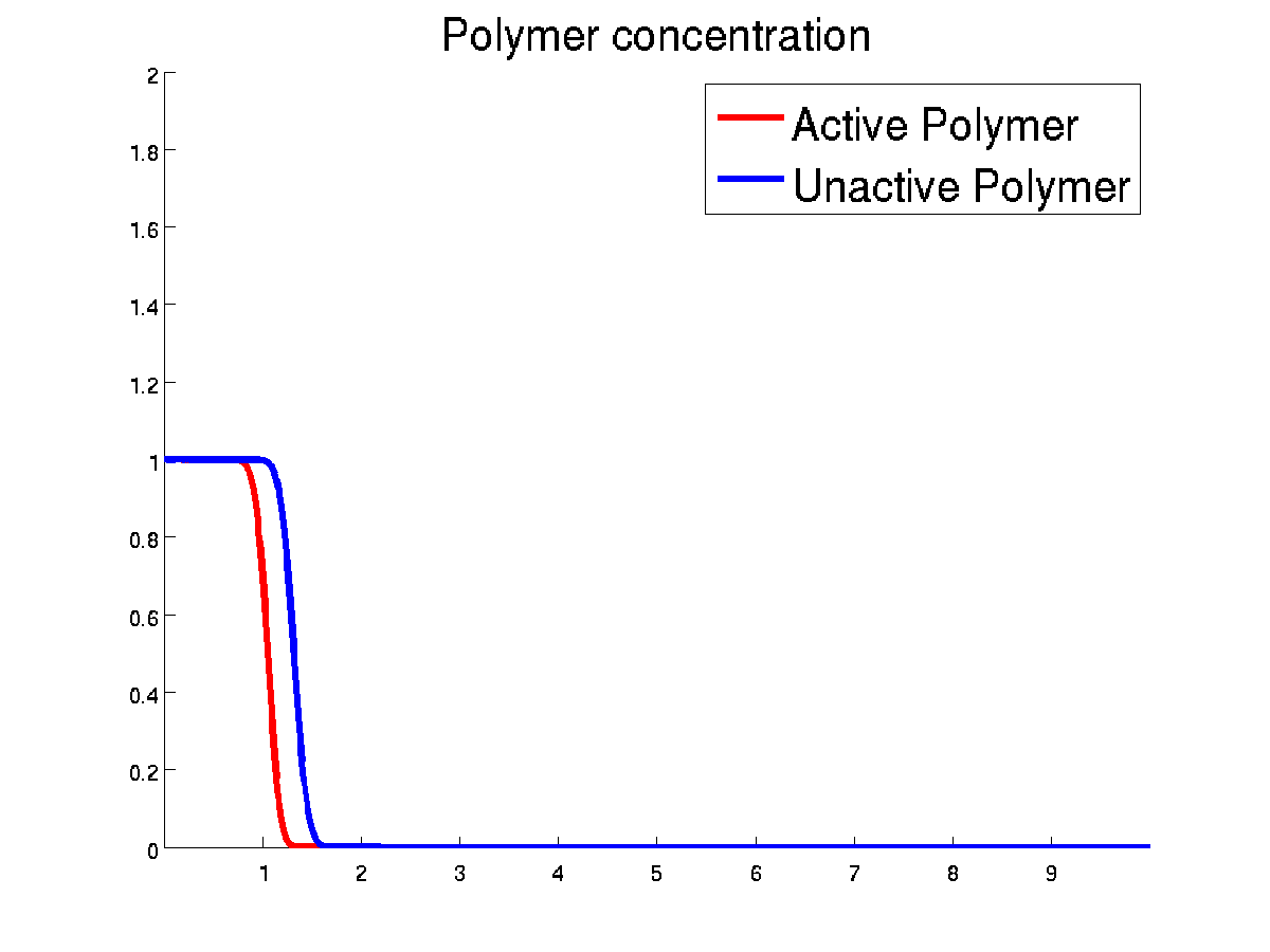
The second solver is implemented from MRST core functionalities. Its purpose is to demonstrate how such a solver can be easily implemented in that way. In particular, the user has a direct and simple access to the modeling equations, which are all contained in the files equationOWPolymer.m and computeMobilities.m. The boundary conditions are physical boundary conditons. The plots below show the result of runLabPolymer.m for two sets of data. The first one is LABPOLYMER.DATA which is the same as the one which is run in the tutorial runLabPolymer.m and the second one is LABPOLYMER2.DATA, which corresponds to an inactive polymer. We call inactive polymer a polymer which has no effect on the flow, which is the case when the values of the polymer properties are set as in LABPOLYMER2.DATA. In such case, the polymer behaves like a tracer. We simulate a one dimensional problem with 1000 cells. We use an explicit solver but an implicit solver is also implemented. The difference between the two solvers is in fact only one line of code in the file equationOWPolymer.m. Initially the water saturation is close to residual saturation and we inject water and polymer with concentration equal to one. we can observe how polymer reduce the water mobility and the creation of a second front for the water propagation. The plot below shows the results of the two simulations at final time.