Simple Polymer simulator

We set up a simple polymer simulator with a cartesian grid and physical boundary conditons such as given influx in input cells and given pressure, saturation and concentration on output faces.

function [G, states] = runLabPolymer()

Add mrst modules which are used

   mrstModule add ad-fi deckformat mrst-gui ad-props

Input data are read from a file. The format is the same as Eclipse. Values are store in the deck structure. The input file contains the fluid and polymer properties.

   current_dir = fileparts(mfilename('fullpath'));
   fn = fullfile(current_dir, 'LABPOLYMER.DATA');
   deck = readEclipseDeck(fn);

The deck variables are converted to SI units. MRST uses exclusively SI units in the computation. Conversion tools are available.

   deck = convertDeckUnits(deck);

Generate grid. We set up two cases: 1D or 2D. The changes in the remaining of the code are minimal. They appear only in the file setupControls.m where the boundary conditions are set.

   sim_case = '1D'; % '1D' or '2D'

   switch sim_case

     case '1D'

       nx = 1000;
       ny = 1;
       nz = 1;

       xlength = 10;
       ylength = 1;
       zlength = 1;

     case '2D'

       nx = 100;
       ny = 100;
       nz = 1;

       xlength = 10;
       ylength = 10;
       zlength = 1;

   end

The function ¦cartGrid¦ generates a MRST unstructured grid. The function computeGeometry computes geometrical properties such as cell volumes, faces areas...

   G = cartGrid([nx ny nz], [xlength, ylength, zlength]);
   G = computeGeometry(G);

Setup rock structure containing the rock properties.

   rock.perm = repmat(100*milli*darcy, [G.cells.num, 1]);
   rock.poro = repmat(0.3, [G.cells.num, 1]);

Setup fluid structure containing the fluid and polymer properties form the deck structure.

   fluid = initDeckADIFluid(deck);

We set off gravity.

   gravity off

Setup adsorption function. There are two options: with or without desorption.

   fluid.effads = @(c, cmax) effads(c, cmax, fluid);

Setup the inputs. They are given as boundary conditions and sources

Injection will done in given cells.

   bc.injection.rate = 0.1/day;
   bc.injection.s = 1;
   bc.injection.c = 1;

pressure, saturation and polymer concentration are imposed on given faces

   bc.dirichlet.pressure = 100*barsa;
   bc.dirichlet.s = 0;
   bc.dirichlet.c = 0;

The function setupControls.m set up the bc structure.

   bc = setupControls(G, bc, sim_case);

The function setupSystem.m sets up the system. In particular, it defines the discrete differential operators.

   system = setupSystem(G, rock, bc);
   system.fluid = fluid;
   system.rock = rock;
   system.nonlinear.tol           = 1e-4;
   system.nonlinear.maxIterations = 30;
   system.nonlinear.relaxRelTol   = 0.2;
   system.cellwise                = 1:3;

The transport part can be either solved explicitly or implicitly. From the implementation point of view, it corresponds to one line of change in the code, see equationOWPolymer.m

   system.implicit_transport = false;

Set up the initial state with constant pressure, saturation and polymer concentration.

   nc = G.cells.num;
   init_state.pressure = 1*atm*ones(nc,1);
   init_state.s        = ones(nc, 1)*[0.2, 0.8];
   init_state.c        = zeros(G.cells.num, 1);
   init_state.cmax     = zeros(G.cells.num, 1);

Compute and store the mobilities for the Dirichlet values

   [bc.mobW, bc.mobO, bc.mobP] = computeMobilities(bc.dirichlet.pressure, ...
                                                   bc.dirichlet.s       , ...
                                                   bc.dirichlet.c       , ...
                                                   bc.dirichlet.c       , ...
                                                   fluid);

Set up time stepping parameters. We use a fixed time step.

   total_time = 2*day;
   dt         = 0.001*day;
   steps      = dt*ones(floor(total_time/dt), 1);
   t          = cumsum(steps);

We start the time step iterations. Each iteration is solved fully implicitly.

Time step iterations.

   state0 = init_state;

   nsteps = numel(steps);
   states = cell(nsteps, 1);

   for tstep = 1 : nsteps

      dt = steps(tstep);

Call non-linear solver solvefi.m to compute next state

      [state, conv, its] = solvefi(state0, dt, bc, system);

      if ~(conv)
         error('Convergence failed. Try smaller time steps.')
         return
      else
         fprintf('Step %d completed in %d Newton iterations\n', tstep, its);
      end

      states{tstep} = state;
      state0 = state;

   end

   plotState(state, G.cells.centroids(:, 1));

end

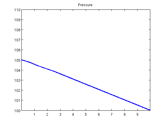
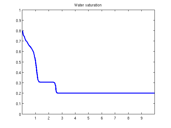
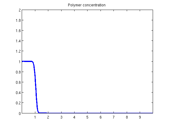
Helper function

function y = effads(c, cmax, f)
   if f.adsInx == 2
      y = f.ads(max(c, cmax));
   else
      y = f.ads(c);
   end
end


function plotState(state, xval)
   figure(1)
   plot(xval, state.pressure/barsa);
   axis([xval(1), xval(end), 100, 110]);
   title('Pressure')
   figure(2)
   plot(xval, state.s(:, 1));
   axis([xval(1), xval(end), 0, 1]);
   title('Water saturation')
   figure(3)
   plot(xval, state.c);
   axis([xval(1), xval(end), 0, 2]);
   title('Polymer concentration')
end