Polymer Simulator

Contents

Add mrst modules which are used

mrstModule add ad-core ad-blackoil ad-fi deckformat ad-props

Input data are read from a file. The format is the same as Eclipse. Values are store in the deck structure.

current_dir = fileparts(mfilename('fullpath'));
fn    = fullfile(current_dir, 'POLYMER.DATA');
deck = readEclipseDeck(fn);

The deck variables are converted to SI units. MRST uses exclusively SI units in the computation. Conversion tools are available.

deck = convertDeckUnits(deck);

Generate grid from deck

G = initEclipseGrid(deck);
G = computeGeometry(G);

Setup rock structure containing the rock properties.

rock  = initEclipseRock(deck);
rock  = compressRock(rock, G.cells.indexMap);

Setup fluid structure containing the fluid properties.

fluid = initDeckADIFluid(deck);

% Oil rel-perm from 2p OW system.
% Needed by equation implementation function 'eqsfiOWExplictWells'.
%

fluid.krO = fluid.krOW;

We include gravity

gravity on

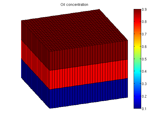
Set up simulation parameters

We want a layer of oil on top of the reservoir and water on the bottom. To do this, we alter the initial state based on the logical height of each cell. The resulting oil concentration is then plotted.

ijk = gridLogicalIndices(G);

state0 = initResSol(G, 300*barsa, [ .9, .1]);
state0.s(ijk{3} == 1, 2) = .9;
state0.s(ijk{3} == 2, 2) = .8;

Enforce s_w + s_o = 1;

state0.s(:,1) = 1 - state0.s(:,2);

Add zero polymer concentration to the state. The cmax variable is necessary for the adsorption model, when desorption is turned off.

state0.c    = zeros(G.cells.num, 1);
state0.cmax = zeros(G.cells.num, 1);

The function setupSimComp sets up the system

s = setupSimComp(G, rock, 'deck', deck);

We plot the oil concentration

figure(1); clf;
plotCellData(G, state0.s(:,2));
plotGrid(G, 'facec', 'none');
title('Oil concentration');
axis tight off
view(70, 30);
colorbar;

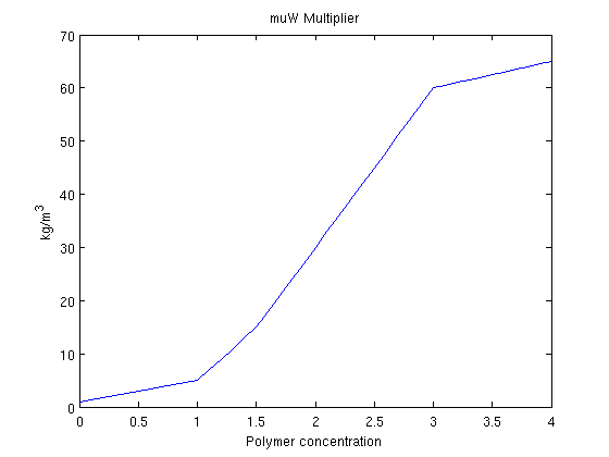
When polymer is added to the water phase, the viscosity of the water phase containing
polymer is increased. Because mobility is defined as the ratio between permeability and
viscosity, this makes the water much less mobile. As a problem with water injection with
regards to oil production is that the water is much more mobile than the hydrocarbons we
are trying to displace, injecting a polymer may be beneficial towards oil recovery.

We plot the viscosity multiplier function fluid.muWMult.

figure(2); clf;
dc = 0:.1:fluid.cmax;
plot(dc, fluid.muWMult(dc))
title('muW Multiplier')
xlabel('Polymer concentration')
ylabel('kg/m^3')

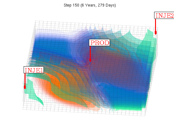
To quantify the effect of adding the polymer to the injected water, we will solve the same system both with and without polymer. This is done by creating both a Oil/Water/Polymer system and a Oil/Water system. Note that since the data file already contains polymer as an active phase we do not need to pass initADISystem anything other than the deck.

modelPolymer = OilWaterPolymerModel(G, rock, fluid, 'inputdata', deck);
modelOW = TwoPhaseOilWaterModel(G, rock, fluid, 'inputdata', deck);

Convert the deck schedule into a MRST schedule by parsing the wells

schedule = convertDeckScheduleToMRST(G, modelPolymer, rock, deck);

We run the simulation. Any options such as maximum non-linear iterations and tolerance can be set in the system struct.

[wellSolsPolymer, statesPolymer] = simulateScheduleAD(state0, modelPolymer, schedule);

[wellSolsOW, statesOW] = simulateScheduleAD(state0, modelOW, schedule);

Plot the schedule

We visualize the schedule and plot both the water, oil and polymer concentration using a simple supplied volume renderer. At the same time we visualize the sum of the oil/water ratio in the producer for both with and without polymer injection in a single pie chart.

W = schedule.control(1).W;
figure(gcf); clf;
view(10,65);
drawnow;

[az, el] = deal(6, 60);

nDigits = floor(log10(numel(statesPolymer) - 1)) + 1;

figure(3); clf;
for i = 1 : numel(statesPolymer) - 1,
    injp  = wellSolsPolymer{i}(3);
    injow = wellSolsOW{i}(3);

    state = statesPolymer{i + 1};

    plotGrid(G, 'facea', 0,'edgea', .05, 'edgec', 'k');
    plotGridVolumes(G, state.s(:,1), 'cmap', @winter, 'N', 10)
    plotGridVolumes(G, state.c,      'cmap', @autumn, 'N', 10)
    plotWell(G, W);
    axis tight off

    cumt = cumsum(schedule.step.val);
    title(sprintf('Step %0*d (%s)', nDigits, i, formatTimeRange(cumt(i))));

    view(az, el);
    drawnow;
end

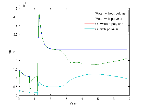
Plot the accumulated water and oil production for both cases

We concat the well solutions and plot the accumulated producer rates for both the polymer and the non-polymer run. The result shows that

figure(4); clf;

wspoly = vertcat(wellSolsPolymer{:});
wsow = vertcat(wellSolsOW{:});

data = -([ [wsow(:,3).qWs]   ; ...
           [wspoly(:,3).qWs] ; ...
           [wsow(:,3).qOs]   ; ...
           [wspoly(:,3).qOs] ] .');
data = bsxfun(@times, data, schedule.step.val);

plot(convertTo(cumt, year), convertTo(data, stb));
legend({'Water without polymer', 'Water with polymer', ...
       'Oil without polymer', 'Oil with polymer'}, 'Location', 'NorthEast');
ylabel('stb');
xlabel('Years');