MRSTlogo_web_banner_light_thinner_Epi.png

MRST-core
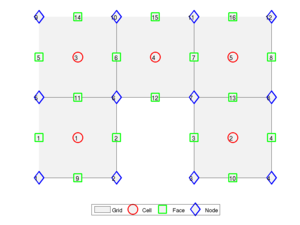
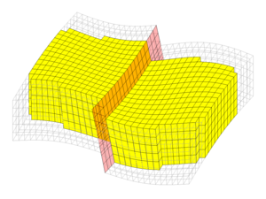
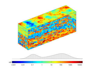
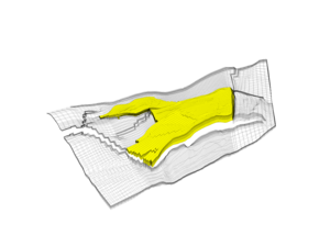
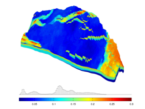
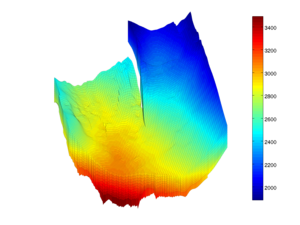
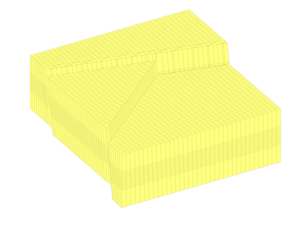
The core module contains routines and data structures for creating and manipulating grids, petrophysical data, and global drive mechanisms such as gravity, boundary conditions, source terms, and wells. The core also contains an implementation of automatic differentiation (you write the formulas and specify the independent variables,the software computes the corresponding derivatives or Jacobians) based on operator overloading, as well as a few routines for plotting cell and face data defined over a grid. The core module is designed to be as minimal as possible.

General overview tutorials

Basic flow tutorial

This example shows the basic steps for setting up, solving, and visualizing a flow problem using the functionality from MRST core and the incomp modules. The flow problem describes vertical equilibrium inside a simple single-phase fluid column. Because of the gravity forces, the pressure will increase linearly downward. The example is very short and gives a quick introduction to MRST.

Read more..


Plotting intro

MRST contains a suite of visualization routines which make it easy to create visualizations of grids and results. This tutorial show how to visualize grids, subsets of grids and details the different routines included in MRST.

Read more..


Basic objects

The most fundamental object in MRST is the grid. This dual purpose object both discretises a model's geometry and serves as a database to which static and dynamic properties and other objects are attached. Examples of such associate data are

    • Static petrophysical properties (e.g., permeability tensor or porosity)
    • Derived properties like transmissibility or pore-volume
    • Dynamic mass distributions (phase saturation and/or concentration of chemical species or tracers)
    • Explicit model partitionings like PVT or relative permeability region mappings
    • Source terms like wells or open boundaries

This example explores a number of ways of constructing grids with degrees of complexity varying from simple Cartesian models with synthetic values for the porosity and permeability through to fully unstructured models in the industry-standard corner-point format. We moreover introduce a collection of open datasets that are either hosted on the MRST website or published on other sites.


Automatic differentiation

Automatic differentiation is, quoting from Wikipedia, "a set of techniques to numerically evaluate the derivative of a function specified by a computer program. AD exploits the fact that every computer program, no matter how complicated, executes a sequence of elementary arithmetic operations (addition, subtraction, multiplication, division, etc.) and elementary functions (exp, log, sin, cos, etc.). By applying the chain rule repeatedly to these operations, derivatives of arbitrary order can be computed automatically, accurately to working precision, and using at most a small constant factor more arithmetic operations than the original program."

The tutorial gives you a brief introduction to MRST's implementation of AD, which is specifically geared towards discretization of partial differential equations and computation with long vectors and sparse matrices. Unlike many other implementations of AD, we have chosen to keep individual Jacobians as a list of sparse matrices and not automatically expand into a large global matrix. This ensures efficiency and flexibility in manipulating matrix blocks corresponding to subequations of (complex) equation systems.


AD flow solver

The purpose of the example is to give the first introduction to how one can use the automatic differentiation (AD) class in MRST to write a flow simulator for a compressible single-phase model. For simplicity, the reservoir is assumed to be a rectangular box with homogeneous properties and no-flow boundaries. Starting from a hydrostatic initial state, the reservoir is produced from a horizontal well that will create a zone of pressure draw-down. As more fluids are produced, the average pressure in the reservoir drops, causing a gradual decay in the production rate.

The example introduces you to the concept of discrete discrete gradient and divergence operators, defined on the grid's interior connections and active cells, respectively. The discrete gradient operator maps from cell pairs to faces and is defined as the difference in the cell values on opposite sides of the face. The discrete divergence operator is a linear mapping from faces to cells and can be computed as the adjoint of the discrete gradient operator. The divergence operator represent the sum of all outgoing fluxes from a cell. Using these operators, we can write flow equations on residual form and then use automatic differentiation to assemble a Jacobi matrix, which is used as part of a Newton loop to solve the nonlinear system of discrete flow equations.


Grid tutorials

Overview of grid factory routines

In this tutorial, we will introduce you briefly to the grid structure and give an overview of some of the many grid factory routines that can be used to generate various types of grids. This includes rectilinear and curvilinear grids, triangulated grids, extruded triangular grids (prismatic), and various hexahedral grids.

Read more..


Rectilinear/curvilinear grids

In this tutorial, we describe how you can use MRST to construct Cartesian and rectilinear grids for rectangular and non-rectangular domains and show how you can populate your grid with petrophysical properties. To this end, we will grid a rectangular domain, from which we cut out a half circle. This example is discussed in more detail in [Jolt 2]


Unstructured grids

In this tutorial, we describe how you can use MRST to construct various kinds of unstructured grids based on Delaunay triangulations and Voronoi diagrams. This example is discussed in more detail in [Jolt 2]


Corner-point grids

In this example we will show several examples how to manipulate and plot corner-point data. As an example, we will use a family of simple models with a single fault, which can be realized in different resolutions.


Tutorials exploring public data sets

MRST provides simple access to a number of public data sets that can be freely downloaded from the internet. The core module contains tutorial examples that explore a few of these data sets in more detail (some examples are also found in the book module).


Model 2 of the 10th SPE Comparative Solution Project

The data set was originally posed as a benchmark for upscaling methods. The 3-D geological model consists of 60x220x85 grid cells, each of size 20ftx10ftx2ft. The model is a geostatistical realization from the Jurassic Upper Brent formations, in which one can find the giant North Sea fields of Statfjord, Gullfaks, Oseberg, and Snorre. In this specific model, the top 70 ft (35 layers) represent the shallow-marine Tarbert formation and the lower 100 ft (50 layers) the fluvial Ness formation. The data can be obtained from the SPE website The data set is used extensively in the literature, and for this reason, MRST has a special module that will download and provide easy access to the data set.


Introduction to the Norne Model

Norne is an oil and gas field lies located in the Norwegian Sea. The reservoir is found in Jurrasic sandstone at a depth of 2500 meter below sea level. Operator Statoil and partners (ENI and Petoro) have agreed with NTNU to release large amounts of subsurface data from the Norne field for research and education purposes. The Norne Benchmark datasets are hosted and supported by the Center for Integrated Operations in the Petroleum Industry (IO Center) at NTNU. Recently, the OPM Initiative released the full simulation model as an open data set on GitHub. In the example, we go through the grid and petrophysical properties from the simulation model.


Introduction to the SAIGUP Model

The SAIGUP (Sensitivity Analysis of the Impact of Geological Uncertainties on Production) project generated a large number of realistic geological models representing shallow marine environments. The developers of MRST have been allowed to publish one specific realization that has faults, inactive cells, disconnected components, but no pinchouts. We will show how to read, process, and visualize the reservoir model and discuss some of the petrophysical properties.


Introduction to the Johansen Aquifer

The Johansen formation was for a period considered as a candidate site for large-scale CO2 storage offshore the south-west coast of Norway. The MatMoRA project has developed a set of geological models based on available seismic and well data. The data set contains four different models: one model of the whole field and three sector models with different vertical resolution. Herein, we will inspect one instance of the model in more detail.


Case B4: fault modelling

There are several ways one can model inclined faults. This examples shows how two inclined, intersecting faults can either be modelled by a stair-stepped hexahedral grid or by a pillar grid in which the pillars are gradually inclined to match the inclination of the fault. The dataset contains realizations with 36x48 or 72x96 cells in the lateral plane for each grid type.


Literature

Published December 8, 2016