Contents

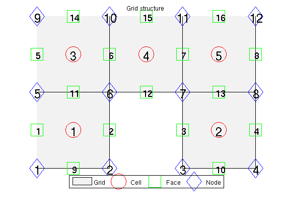
Create a 2D grid

We start by creating a simple 2D Cartesian grid. We then remove one cell and add geometry information to the resulting grid.

G = cartGrid([3,2]);
G = removeCells(G, 2);
G = computeGeometry(G);

Plot cell, face, and node numbers

newplot;
% Plot the grid
plotGrid(G,'FaceColor',[0.95 0.95 0.95]); axis off;
hold on;

% To improve readability, we extract the cell and face centroids as well as
% the coordinates of each node. These will be used for plotting the cells,
% faces and node indices respectively.
c_cent = G.cells.centroids;
f_cent = G.faces.centroids;
coords = G.nodes.coords;

% Add circles around the centroids of each cell
plot(c_cent(:,1), c_cent(:,2),'or','MarkerSize',24);

% Plot triangles around face centroids
plot(f_cent(:,1), f_cent(:,2),'sg','MarkerSize',24);

% Plot squares around nodes
plot(coords(:,1), coords(:,2),'db','MarkerSize',24);

legend({'Grid', 'Cell', 'Face', 'Node'}, 'Location', 'SouthOutside', 'Orientation', 'horizontal')

% Plot cell/face centroids and nodes
text(c_cent(:,1)-0.04, c_cent(:,2), num2str((1:G.cells.num)'),'FontSize',20);
text(f_cent(:,1)-0.045, f_cent(:,2), num2str((1:G.faces.num)'),'FontSize',16);
text(coords(:,1)-0.075, coords(:,2), num2str((1:G.nodes.num)'),'FontSize', 18);

title('Grid structure')
hold off;

Finding mappings between grid primitives

The unstructured grid is built upon coordinates representing nodes, nodes representing faces and faces representing cells. To save memory, some attributes are run length encoded. For more information, see 'help grid_structure'. For instance, let us look up information for the faces.

faces =[ rldecode(1 : G.cells.num,diff(G.cells.facePos), 2).' G.cells.faces];
tag = {'West'; 'East'; 'South'; 'North'; 'Bottom'; 'Top'};
fprintf('Cell\tFace\tTag id\tTag\n');
for i=1:size(faces,1)
   fprintf(' %3d\t%3d\t%3d\t[%s]\n', faces(i,1:3), tag{faces(i,3)});
end

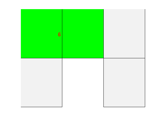
Cell	Face	Tag id	Tag
   1	  1	  1	[West]
   1	  9	  3	[South]
   1	  2	  2	[East]
   1	 11	  4	[North]
   2	  3	  1	[West]
   2	 10	  3	[South]
   2	  4	  2	[East]
   2	 13	  4	[North]
   3	  5	  1	[West]
   3	 11	  3	[South]
   3	  6	  2	[East]
   3	 14	  4	[North]
   4	  6	  1	[West]
   4	 12	  3	[South]
   4	  7	  2	[East]
   4	 15	  4	[North]
   5	  7	  1	[West]
   5	 13	  3	[South]
   5	  8	  2	[East]
   5	 16	  4	[North]

Neighborship is defined through faces

G.faces.neighbors(i,:) contains the cells neighboring to face i. We define a new grid and plot the neighbors of face 10 in the new grid. G = cartGrid([3,3,1]);

clf;
plotGrid(G,'FaceAlpha', 1, 'FaceColor', [0.95 0.95 0.95]); axis off;

f = 6;
plotGrid(G, G.faces.neighbors(f,:), 'FaceColor', 'Green')
text(f_cent(f,1)-0.1, f_cent(f,2), num2str(f),'FontSize',16,'Color','red');
% This also defines the boundary faces, since faces with only one neighbor
% is on the edge of the domain:
boundary = any(G.faces.neighbors==0,2);
facelist = 1:G.faces.num;
fprintf('Boundary faces: \n')
facelist( boundary) %#ok intentional display
fprintf('Internal faces: \n')
facelist(~boundary) %#ok intentional display

Boundary faces: 

ans =

     1     2     3     4     5     8     9    10    12    14    15    16

Internal faces: 

ans =

     6     7    11    13

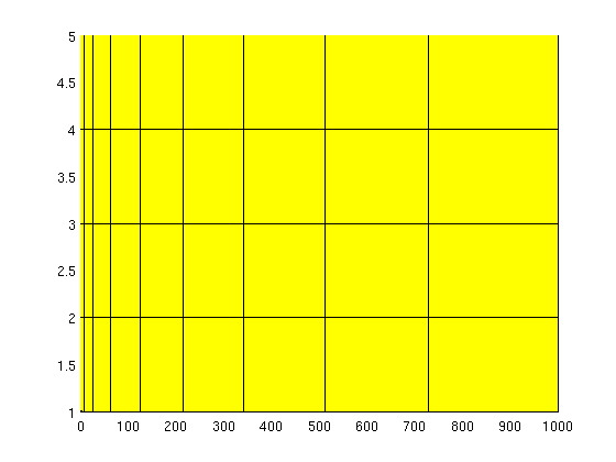
Generating synthethic grids using MRST

There are many options for creating synthethic grids in MRST. For instance, the simple cartGrid already shown is a special case of tensorGrid:

G = tensorGrid((1:10).^3, 1:5);

clf;
plotGrid(G);

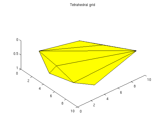
Triangulated grids

We can generate a triangulated grid using existing triangulations, from MATLAB or elsewhere.

% Generate points
pts = rand(20,3).*repmat([10,10,1], 20, 1);
% Triangulate
T = DelaunayTri(pts(:,1), pts(:,2), pts(:,3));


G = tetrahedralGrid(pts, T.Triangulation);
clf;
title('Tetrahedral grid')
plotGrid(G);
view(50,60)

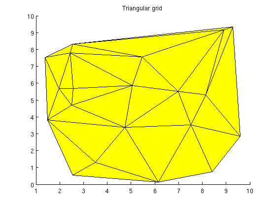
Triangular grids

Generate a 2D triangle grid from the same data using the xy-coordinates

pts_2d = pts(:,1:2);
% Triangulate
T_tri = DelaunayTri(pts_2d(:,1), pts_2d(:,2));
G_tri = triangleGrid(pts_2d, T_tri.Triangulation);

clf
title('Triangular grid')
plotGrid(G_tri);

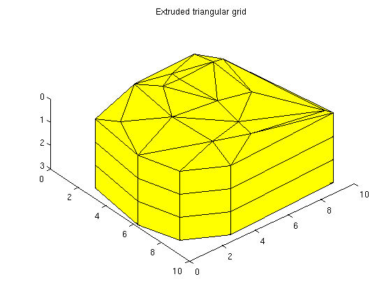
Extruded grid

If we have an interesting 2D grid, we can easily extend it to 3D by using makeLayeredGrid. We will extend the previous triangle grid to 3 layers

G = makeLayeredGrid(G_tri, 3);
clf;
title('Extruded triangular grid')
plotGrid(G);
view(50,60)

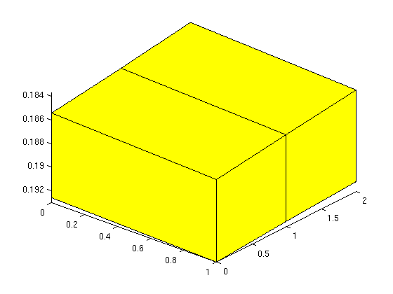
Explicit hexahedral grid

Hexahedral grids can also be generated by lists of nodes and node indices. For valid node ordering, see help hexahedralGrid

H = [1  2  3  4  5  6  7  8; ... % Cell 1
    2  9 10  3  6 11 12  7]; ... % Cell 2


P = [  1  0  0.1860; ...
       1  1  0.1852; ...
       1  1  0.1926; ...
       1  0  0.1930; ...
       0  0  0.1854; ...
       0  1  0.1846; ...
       0  1  0.1923; ...
       0  0  0.1926; ...
       1  2  0.1844; ...
       1  2  0.1922; ...
       0  2  0.1837; ...
       0  2  0.1919]; ...

 G = hexahedralGrid(P, H);

 clf;
 plotGrid(G);
 axis tight
 view(40,40)

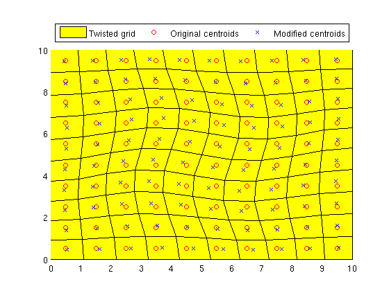
Grids can be manipulated after creation

We can alter the attributes of a grid after creation. In this example we twist the grid slightly. One caveat: Any computed properties of the grid will not be altered. For instance, computeGeometry must be called again after grid updates to get correct cell centroids.

G = cartGrid([10, 10]);
G_before = computeGeometry(G);
% Twist the coordinates to create a non-K-orthogonal grid.
G_after = twister(G);
G_after = computeGeometry(G_after);
clf;
plotGrid(G_after);
hold on
plot(G_before.cells.centroids(:,1), G_before.cells.centroids(:,2), 'Or')
plot(G_after.cells.centroids(:,1), G_after.cells.centroids(:,2), 'xb')
legend('Twisted grid', 'Original centroids', 'Modified centroids', ...
       'Location', 'NorthOutside', 'Orientation', 'horizontal')

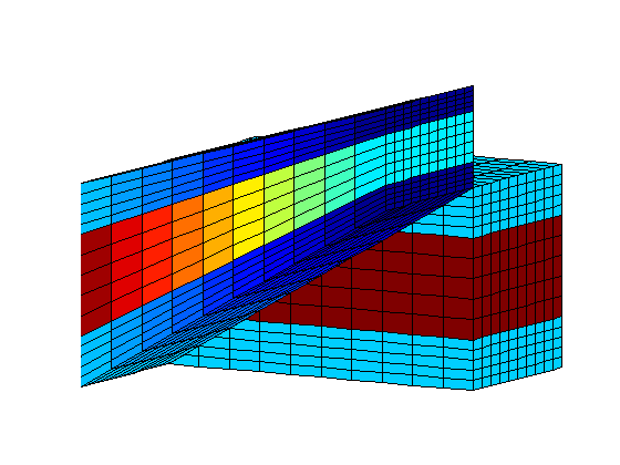
Some grid routines produce GRDECL structures

These can be converted to MRST grids using processGRDECL, just as one would with a GRDECL file read using readGRDECL. For instance, here is a three layered structure which is easy to generate by creating pillars manually.

G = processGRDECL( threeLayers(10,10,5));
G = computeGeometry(G);
clf;
% Color the cells by the cell volume to show the layered structure.
plotCellData(G, G.cells.volumes,'EdgeColor','k');
view(120,10);
axis tight off

simpleGrdecl can generate different grids based on optional parameters

Generate three grids using the same function

grdecl = simpleGrdecl([20, 20, 5]);
G1 = processGRDECL(grdecl);

grdecl = simpleGrdecl([20, 20, 5], @(x) 0.05 * (sin(2*pi*x) - 1.5));
G2 = processGRDECL(grdecl);

grdecl = simpleGrdecl([20, 20, 5], @(x) 0.25*(x-0.5), 'flat', true);
G3 = processGRDECL(grdecl);

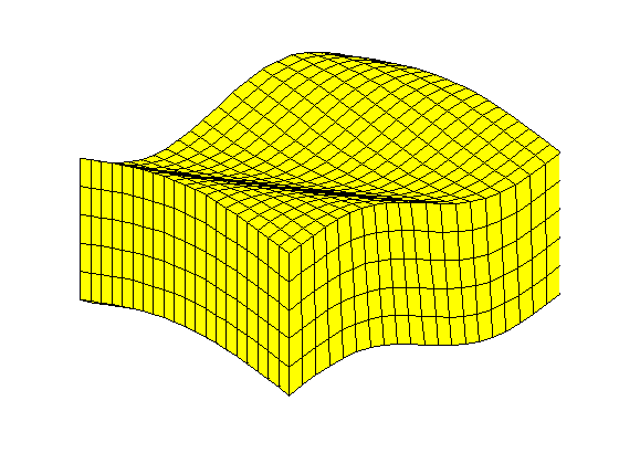
simpleGrdecl - default parameters

The default parameter gives a simple, wavy grid.

clf;
plotGrid(G1)
view(3);
axis tight off;

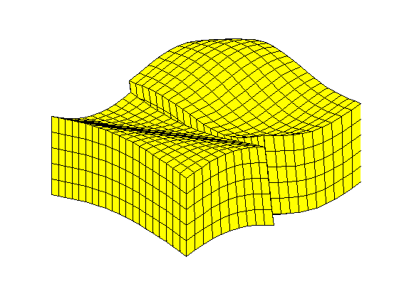
simpleGrdecl - with a function handle

By supplying a function handle, the grid becames faulted based on the values of the function at the fault line.

clf;
plotGrid(G2)
view(3);
axis tight off;

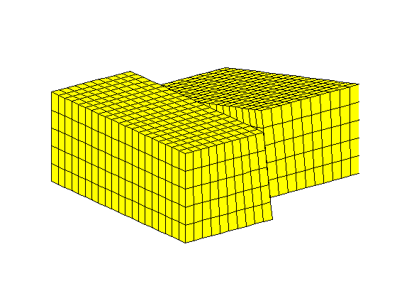
simpleGrdecl - flat with linear fault

Create a flat grid with another fault function

clf;
plotGrid(G3)
view(3);
axis tight off;