You are here:
MRST
/
Documentation
/
Tutorials
/
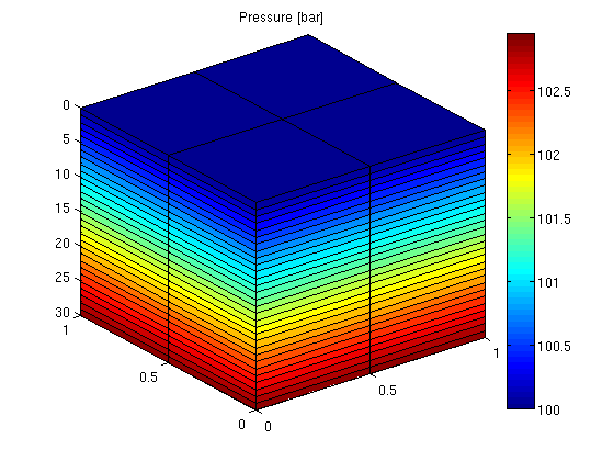
Gravity Column
![$$\nabla\cdot v = q, \qquad v=\textbf{--}\frac{K}{\mu} \bigl[\nabla p+\rho g\nabla z\bigr],$$](/globalassets/project/mrst/imgs/tutorial/imgs/gravitycolumn_eq82190.png)