
Introduction
exploreSimulation is an interactive tool for setting up and simulating long-term, aquifer-wide CO2 storage scenarios, applied on real datasets of geological formations in the Norwegian North Sea. The simulation is based on the vertical equilibrium assumption, which allows for rapid simulations even for large temporal and spatial domains. The simulated outcome of thousands of years of CO2 migration can usually be obtained within minutes.
The application covers the whole value chain from setting up an injection/migration scenario, running the simulation and visualising the outcome. It also keep track of the CO2 trapping state at any given time of the simulation. This information is used to produce CO2 inventories, which is a way to graphically display how CO2 state in the aquifer evolves during the simulation period.
Workflow in a nutshell
The application is designed for ease of use. The user begins by choosing a geological formation from a list of available alternatives. Then he/she specifies boundary conditions, injection sites, injection rates, durations and physical effects. After launching the simulation, progress can be tracked in a separate visualisation window. When simulation is completed, the resulting CO2 inventory is presented. The visualization window can also be used to plot the value of a number of variables (CO2 saturation, pressure, etc.) for any timestep of the simulation. The outcome can also be saved to disk.
A number of simulations with different input parameters can be launched from the scenario specification window, each being assigned its own visualization window.
Despite its simplicity and low compuational requirements, the simulator is capable of taking a significant range of physical effects into account, including realistic fluid properties (based on accurate equation of states), rock properties (relative permeability, capillary effects, compressibility), two-phase flow, CO2 dissolution into brine, residual saturation, and structural trapping on macro and subscale levels. There are three different types of boundary conditions, all of which can be applied on different parts of the boundary for any given simulation.
Launching the application
First, ensure that the geological datasets have been downloaded. This can be done in a semi-automatic fashion by launching the graphical dataset download manager as follows:
mrstDatasetGUI;
Choose the CO2Atlas entry from the menu on the left and click the Download button. These public datasets are provided by the Norwegian Petroleum Directorate. (We further discuss their use with MRST-CO2lab here).
The simulation tool is launched by ensuring the co2lab module is loaded and simply typing its name:
mrstModule add co2lab; % ensure that the co2lab module is loaded
exploreSimulation;     % run the application
The exploreSimulation command can take additional arguments to change various parameters that are not necessarily available through the graphical user interface. For details, refer to this section.
Specifying a scenario
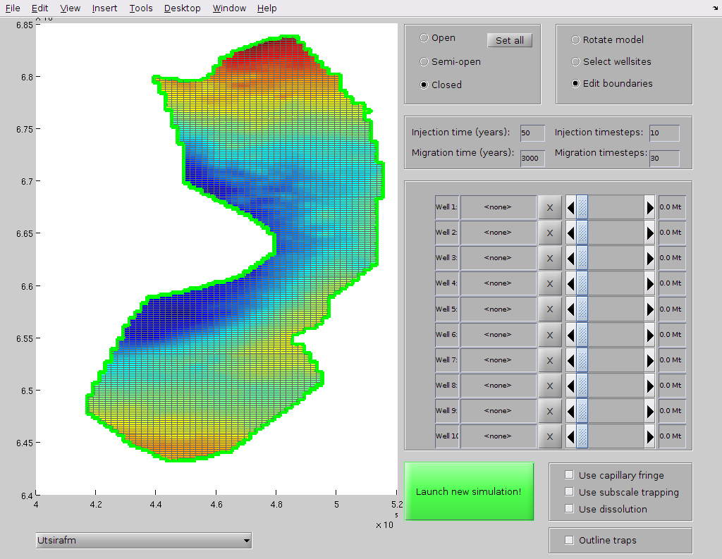
Figure 1: Scenario specification interface (click in image for full-size version)
Upon launching the application, the user is presented with the interface displayed in Figure 1. This is the scenario specification interface, where the user defines all necessary information for launching a specific injection and migration scenario.
The components of this interface are explained below, presented as a a step-by-step description on how a scenario is specified.
Selecting and displaying a formation
First, the user chooses the desired formation model from the drop-down list at the lower left side of the interface window. The default formation is Utsira ("Utsirafm"), but there are sixteen different formations to choose from. All models represent formations located below the Norwegian North Sea.
The chosen formation will immediately be displayed in the graphical window on the left side of the scenario specification interface. The model can be rotated and visually inspected as long as the "Rotate model" radio button box is selected (located at the upper right corner of the interface). The user has the option to highlight the location of structural traps by ticking the "Outline traps" checkbox found in the lower right corner of the interface.
When rotating the model, it will appear to have no thickness. In fact, only the caprock shape is displayed. The full aquifer thickness will however be taken into account during simulation.
Specifying boundary conditions
Each part of the lateral boundaries of the aquifer must be one of three types: open, semi-open, or closed:
- open: fluids flow freely across this boundary, without any resistance.
- semi-open: fluids flow across this boundary, but with an additional resistance equivalent to flow through an additional distance outside the simulation domain, using the same permeability value as in the aquifer (default distance is 100 km, but this is configurable).
- closed: no flow occurs across this boundary.
In order to specify boundaries, the user must first activate the "Edit boundary" radio button found in the upper right panel of the interface. The default is open boundaries everywhere (indicated as a thick green aquifer outline in the display window). If a completely closed or semi-open boundary is desired instead, the user may select the appropriate radio button in the upper middle panel, and then click "Set all". Semi-open and closed boundaries are drawn with yellow and red lines, respectively.
Boundary conditions may also be defined piecemeal by clicking with the mouse pointer inside the aquifer model. The first click will set a marker (indicated as a red star) at the given position. A second click away from the first will define a line. The part of the boundary closest to this line will change status to whatever condition is active in the upper middle display (open, semi-open or closed). This way, detailed boundary conditions can be set up in an intuitive way even for aquifers with complex boundaries.
Specifying injection (well) locations and rates
It is possible to define up to ten injection locations for a given simulation scenario. Injection locations are chosen by first activating the "Select wellsite" radiobutton in the upper right panel, and then clicking at the desired locations on the model. The location of the well will be indicated with a black dot.
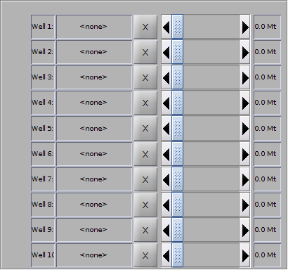
Figure 2: The well table
The injectors will be named W1 to W10. Each injector will be assigned a row in the well table, located in the middle right part of the user interface. When a injector is placed, its row in the well table will become active. Its latitude/longitude coordinates will appear in the second field, and its annual injection rate can be adjusted with the slider (from 0 to 10 megatons per year). An erroneously placed injector can be deleted by clicking the button labeled X in its corresponding row.
Specifying simulation time
On the right hand side of the user interface, there is a small box which allows specifying the duration of the injection (default: 50 years), the duration of the migration phase (default 3000 years), and the number of discrete timesteps used to represent each of these periods. The user is free to play around with these numbers, but should keep in mind that a too small timestep size will just lead to a waste of computing resources, and too large steps may lead to 'timestep cutting', which is also computationally wasteful. In general, the migration phase admits longer timesteps than the injection phase.
Other parameters
On the right of the green 'Launch' button, there is a small box where the user is allowed to select which additional physical effects to include in the simulation. These options are:
- Capillary fringe - The interface between CO2 and brine will not be modeled as a sharp line, but as a diffuse transition from one phase to the other. This may have a significant impact on plume migration.
- Subscale trapping - Take into account the structural trapping that occurs below the resolution of the simulation grid. Further information can be found in publications 2, 3 and 9 from the literature list at the bottom of this page.
- Use dissolution - Take into account the dissolution of CO2 into brine (if left unchecked, the phases will be considered immiscible).
Launch
When the above steps have been taken care of, the scenario is completely specified, and the simulation can be launched by clicking on the green button labeled "Launch new simulation!".
Running the simulation and analysing the outcome
NB: During the simulation process, diagnostic information will be shown in the Matlab shell. This may include warnings such as "Solver did not converge, cutting timestep". This is to be expected, and should not be a cause of worry.
Visualising the result
Once a simulation is launched, a new window opens, presenting user with the result visualization interface.
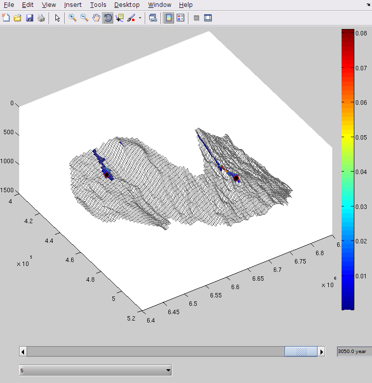
Figure 3: Tool for visual inspection of simulation result
As soon as the simulation is finished, the user can use the slider to move to any timestep in the simulation. Different visualization variables can be chosen from the drop-down menu, including:
s: CO2 saturation (default)pressure: fluid pressure in the aquifersGmax: Historical maximum CO2 saturationh: CO2 plume height (closely related to saturation in a vertical-equilibrium setting)plume_s_avg: The average saturation within the free plume, as a fraction of maximum achievable saturation. For a simulation without capillary effect (sharp-interface), this value will remain constant, but if a capillary fringe is included, this number yield insight on the local significance of the fringe.overpressure: fluid overpressure in the aquifer, defined as the difference between current pressure and initial pressure.
For a better view, the result visualization window can be resized, and the model can be rotated using the rotation button found in the toolbar.
Tracking CO2 state over time
The CO2 inventory display also opens when a simulation has completed. The inventory display tracks the trapping state of CO2 over the course of the simulated (injection and migration) period. For any given year, the inventory shows how much CO2 is found in each of the following states:
- Dissolved : CO2 that has dissolved into brine. (Only available if "Use dissolution" was selected when the scenario was specified).
- Structural residual : CO2 that is both structurally and residually trapped (i.e. residually trapped CO2 within a structural trap).
- Residual : CO2 that is residually trapped, outside structural traps, and not in the free plume.
- Residual in plume: CO2 that is currently part of the free plume, but is destined to be left behind as residual saturation after the imbibition process has been fully completed.
- Structural subscale : CO2 that is caught in structural traps too small to be captured by the grid's resolution. (Only available if "Use subscale trapping" was selected when the scenario was specified).
- Structural plume : Structurally trapped CO2 other than "Structural residual".
- Free plume : CO2 that is free to migrate.
- Exited : CO2 that has left the simulation domain (through an open or semi-open boundary).
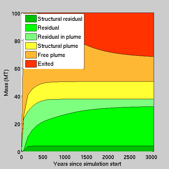
Figure 4: CO2 inventory
Parameters adjustable at startup
To limit the complexity of the user interface, many adjustable parameters can only be specified at the command line when the program is launched. Additional parameters are specified on the form:
exploreSimulation('param1', value1, 'param2', value2, .., 'paramN', valueN)
where 'param1', 'param2' etc. are the names of the parameters to be specified, and value1, value2, etc. are the corresponding values.
Possible parameters that can be specified at the command line are:
grid_coarsening- the extent of downsamping of the grid. A value of 1 means that no downsampling is used, higher values yield progressively coarser grid. Default value is 4. Finer grids leads to simulations that are more computationally expensive.default_formation- name of the formation to load at startup. Default is 'Utsirafm'. (Other possible names can be found in the application's drop-down menu where the active formation is selected).window_size- Size of the application window, in pixels. Default is [1024 768].seafloor_depth- Depth of the sea floor, in meters. Default is 100 m.seafloor_temp- Temperature at sea floor, in °C. Default is 7°.temp_gradient- Temperature gradient, in °C/km depth. Default is 35.6°C/km.water density- Density of brine, in kg/m3. Default is 1000.dis_max- Maximum dissolvable CO2 in terms of volume of CO2 at reference conditions per volume of brine. Default is 0.07 which, using a reference density of 760 kg/m3, corresponds to a dissolution of 53 kg of CO2 per cubic meter of brine.max_num_wells- maximum number of inejector sites allowed. Default value is 10.default_rate- default injection rate for a newly placed well, in terms of volume of CO2 at reference conditions. Default value is 1 megaton divided by the reference density of 760 kg/m3.max_rate- Maximum allowed injection rate, in terms of volume of CO2 at reference conditions. Default value is 10 megatons, divided by the reference density of 760 kg/m3.water_compr_val- Linearized compressibility of water. Default value is 4.3e-10.pvMult- "pore volume multiplier". Expresses the linear compressibility of the rock matrix. Default value is 1e-10.water_residual- Residual saturation of brine, as fracture of pore space. Default value is 0.11.co2_residual- Residual saturation of CO2, as fracture of pore space. Default value is 0.21.inj_time- Duration of the injection period. Default is 50 years.inj_steps- Number of simulation timesteps used to represent the injection period. Default is 10.mig_time- Duration of the migration period, following the injection period. Default is 3000 years.mig_steps- Number of simulation timesteps used to represent the migration period. Default is 30.well_radius- Radius of the wellbore. Default is 0.3 meters.C- Scaling factor for a Brooks-Corey capillary pressure curve (only relevant when the capillary fringe option is utilized). Default value is 0.1.subtrap_file- Name of file containing information on the estimated subscale trapping capacity. Default is 'utsira_subtrap_function_3.mat'.outside_distance- A fictive distance used to compute the flow resistance across semi-open boundaries. Default is 100 kilometers.savefile- The simulation outcome will be saved to the file whose name is given by this variable. If left empty (default), the simulation outcome will not be saved.