Here we show how to do the plotting in the Realistic Syntetic Aquifer tutorial.

Contents

Prepare plotting

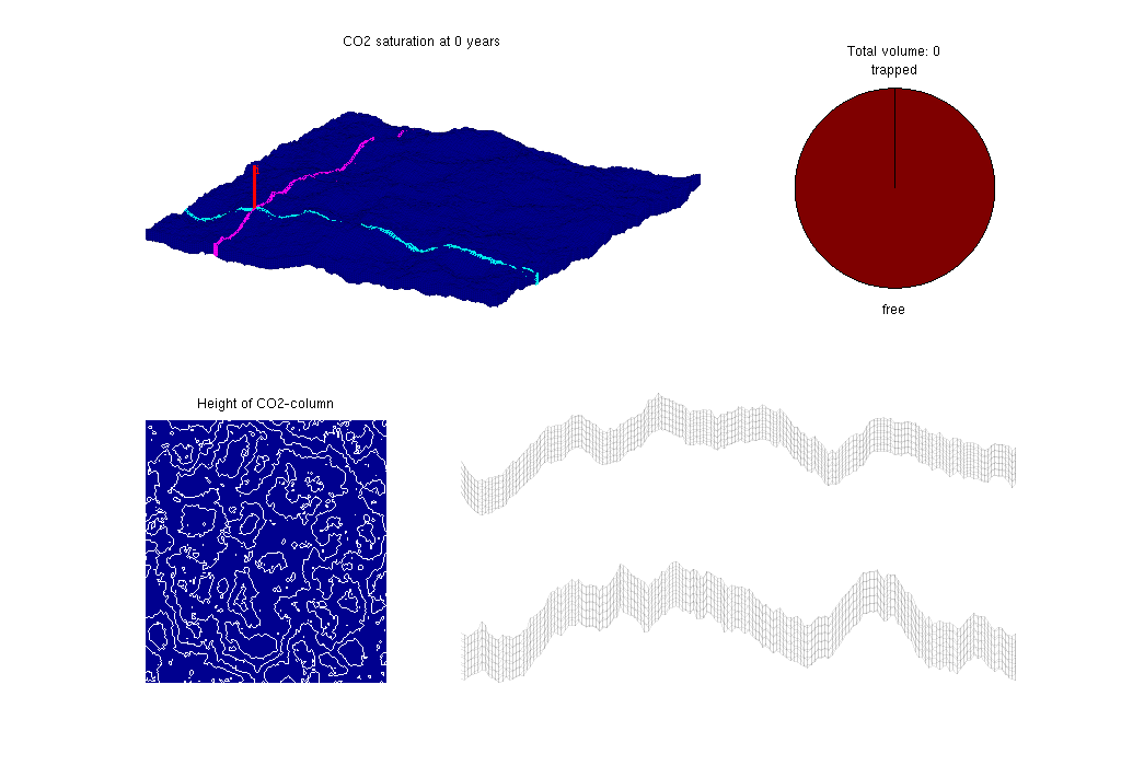
% Extract grid to represent the 2D cross-sections
clear ijk
[ijk{1:3}] = ind2sub(G.cartDims, G.cells.indexMap);
ijk = [ijk{:}];

cells_sub_x = find(ijk(:,2) == wellIx(2));
G_x = extractSubgrid(G, cells_sub_x);
G_x = computeGeometry(G_x);
G_x.cartDims = G.cartDims;

cells_sub_y = find(ijk(:,1) == wellIx(1));
G_y = extractSubgrid(G, cells_sub_y);
G_y = computeGeometry(G_y);
G_y.cartDims = G.cartDims;

% Saturation plotted in a 3D grid with the x- and y-slices outlined in cyan
% and magenta colours, respectively.
clf

% Make sure the white countour lines in the figure stay white when the
% figure is exported to *.png by pre-setting the background color to white
set(gcf, 'color', 'white');

subplot(2,3,1:2);
  sol.s = height2Sat(sol, Gt, fluidVE);
  hsVE1 = plotCellData(G, sol.s, 'EdgeColor','k','EdgeAlpha', 0.05);
  plotGrid(G_x, 'FaceColor', 'none', 'EdgeColor', 'c');
  plotGrid(G_y, 'FaceColor', 'none', 'EdgeColor', 'm');
  plotWell(G, W, 'height', 1000, 'color', 'r');
  title(['CO2 saturation at ', num2str(convertTo(0,year)), ' years']);
  view(30,60); axis tight off
  caxis([0 1-fluidVE.sw]);

% Pie chart of trapped and free CO2
subplot(2,3,3);
  pie([eps 1],{'trapped','free'});
  title('Total volume: 0');

% Height of the CO2 plume plotted on the 2D top-surface grid.
subplot(2,3,4);
  x = reshape(Gt.nodes.coords(:,1),Gt.cartDims+1);
  y = reshape(Gt.nodes.coords(:,2),Gt.cartDims+1);
  hplot = reshape(sol.h(:,1),Gt.cartDims);
  hplot = hplot([1:end end],:);
  hplot = hplot(:,[1:end end]);
  pcolor(x,y,hplot); shading flat;
  hold on,
  contour(x,y,reshape(Gt.nodes.z,Gt.cartDims+1),5,'w')
  hold off, axis tight off
  title('Height of CO2-column');

% Saturation along the x-slice
subplot(4,3,8:9);
  plotGrid(G_x,'FaceColor','none','EdgeAlpha',0.05);
  axis tight off, view([0 0])

% Saturation along the y-slice
subplot(4,3,11:12);
  plotGrid(G_y,'FaceColor','none','EdgeAlpha',0.05);
  axis tight off, view([90 0]), drawnow,

Plotting in simulation loop

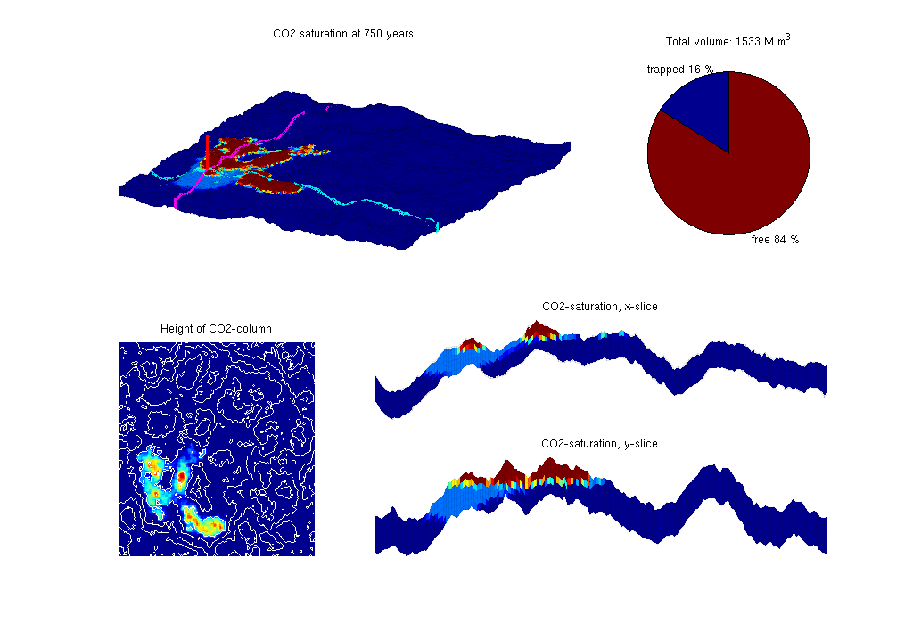
if mod(t,dTplot)~= 0, continue; end
   set(0,'CurrentFigure',figVE);
   subplot(2,3,1:2);
     delete(hsVE1);
     hsVE1 = plotCellData(G, sol.s, 'EdgeColor','k','EdgeAlpha', 0.05);
     title(['CO2 saturation at ', num2str(convertTo(t, year)), ' years']);
     caxis([0 1-fluidVE.sw]);
   subplot(2,3,3);
     str1 = ['trapped ' num2str(round(trappedVol/totVol*100)) ' %'];
     str2 = ['free ' num2str(round(freeVol/totVol*100)) ' %'];
     pie([max(trappedVol,eps) freeVol],{str1, str2});
     title(['Total volume: ', ...
        num2str(round(convertTo(totVol,mega*meter^3))),' M m^3']);
   subplot(2,3,4); cla,
     hplot = reshape(sol.h(:,1),Gt.cartDims);
     hplot = hplot([1:end end],:);
     hplot = hplot(:,[1:end end]);
     pcolor(x,y,hplot); shading flat; caxis([0 max(hplot(:))]);
     hold on,
     contour(x,y,reshape(Gt.nodes.z,Gt.cartDims+1),5,'w')
     hold off, axis tight off
     title('Height of CO2-column');
   subplot(4,3,8:9); cla
     plotCellData(G_x, sol.s(cells_sub_x),'EdgeColor','k','EdgeAlpha',0.05);
     axis tight off, view([0 0])
     title('CO2-saturation, x-slice');
   subplot(4,3,11:12); cla
     plotCellData(G_y, sol.s(cells_sub_y),'EdgeColor','k','EdgeAlpha',0.05);
     axis tight off, view([90 0])
     title('CO2-saturation, y-slice');
   drawnow

Published with MATLAB® 7.10