In this example we consider a synthetic sloping aquifier created in the IGEMS-CO₂ project. The dataset in this example is available for download on this page.

We demonstrate the use of C-accelerated MATLAB, using the functions

see the release notes of MRST 2011a for details.

Contents

Video of simulation

Construct stratigraphic and petrophysical model

addpath(fullfile(ROOTDIR,'mex','libgeometry'));

% Read data
grdecl = readGRDECL(fullfile(ROOTDIR, 'data', 'igems', ...
                   'IGEMS.GRDECL')); 

% Map from left-hand to right-hand coordinate system and process grid
lines = reshape(grdecl.COORD,6,[]);
lines([2 5],:) = -lines([2 5],:);
grdecl.COORD = lines(:); clear lines
G = processgrid(grdecl); toc

% Compute geometry, adding tags needed by topSurfaceGrid
G = mcomputeGeometry(G); toc
G.cells.faces = [G.cells.faces, repmat((1:6).', [G.cells.num, 1])];
rock = grdecl2Rock(grdecl);
rock.perm = convertFrom(rock.perm, milli*darcy);
clear grdecl

% Top-surface grid
disp(' -> Constructing top-surface grid'); 
[Gt, G] = topSurfaceGrid(G); 
rock2D  = averageRock(rock, Gt);

Set time and fluid parameters

T          = 750*year();
stopInject = 150*year();
dT         = 1*year();
dTplot     = 2*dT;

% Make fluid structures, using data that are resonable at p = 300 bar
fluidVE = initVEFluid(Gt, 'mu' , [0.056641 0.30860] .* centi*poise, ...
   'rho', [686.54 975.86] .* kilogram/meter^3, ...
   'sr', 0.2, 'sw', 0.1, 'kwm', [0.2142 0.85]);
gravity on

Set well and boundary conditions

We use one well placed down the flank of the model, perforated in the bottom layer. Injection rate is 2.8e4 m^3/day of supercritical CO₂. Hydrostatic boundary conditions are specified on all outer boundaries.

% Set well in 3D model
wellIx = [G.cartDims(1:2)/5, G.cartDims([3 3])];
rate   = 2.8e4*meter^3/day;
W      = verticalWell([], G, rock, wellIx(1), wellIx(2), ...
                      wellIx(3):wellIx(4), 'Type', 'rate', 'Val', rate, ...
                      'Radius', 0.1, 'comp_i', [1,0], 'name', 'I');

% Well in 2D model
wellIxVE = find(Gt.columns.cells == W(1).cells(1));
wellIxVE = find(wellIxVE - Gt.cells.columnPos >= 0, 1, 'last' );
WVE      = addWell([], Gt, rock2D, wellIxVE, ...
                   'Type', 'rate','Val',rate,'Radius',0.1);

% BC in 2D model
i = any(Gt.faces.neighbors==0, 2);  % find all outer faces
I = i(Gt.cells.faces(:,1));         % vector of all faces of all cells, true if outer
j = false(6,1);                     % mask, cells can at most have 6 faces,
j(1:4)=true;                        %   extract east, west, north, south
J = j(Gt.cells.faces(:,2));         % vector of faces per cell, true if E,W,N,S
bcIxVE = Gt.cells.faces(I & J, 1);
bcVE = addBC([], bcIxVE, 'pressure', ...
            Gt.faces.z(bcIxVE)*fluidVE.rho(2)*norm(gravity));
bcVE = rmfield(bcVE,'sat');
bcVE.h = zeros(size(bcVE.face));


% for 2D/vertical average, we need to change defintion of the wells
for i=1:numel(WVE)
   WVE(i).compi=NaN;
   WVE(i).h = Gt.cells.H(WVE(i).cells);
end

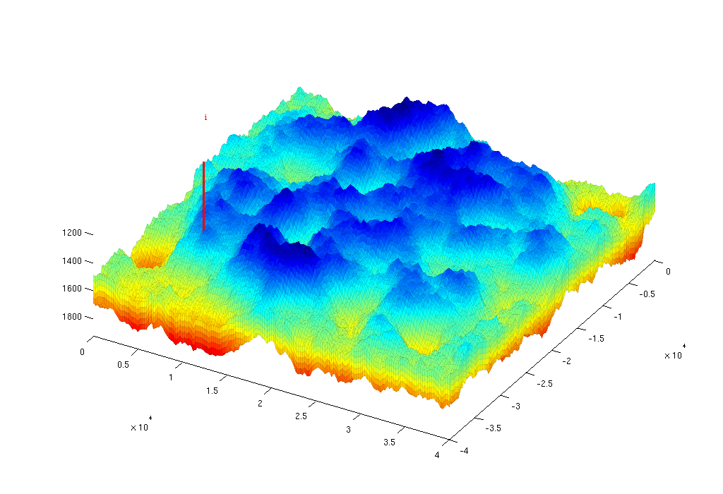
Create figure and plot height and well

scrsz  = get(0,'ScreenSize');
figVE = figure('Position',[scrsz(3)-1024 scrsz(4)-700 1024 700]);
set(0,'CurrentFigure',figVE);
plotCellData(G,G.cells.centroids(:,3),'EdgeColor','k','EdgeAlpha',0.05);
view([30 60]), axis tight;
plotWell(G, W, 'height', 1000, 'color', 'r'); drawnow

Prepare simulations

Compute inner products and instantiate solution structure

SVE = computeMimeticIPVE(Gt, rock2D, 'Innerproduct','ip_simple'); toc
preComp = initTransportVE(Gt, rock2D);
sol = initResSol(Gt, 0);
sol.wellSol = initWellSol(W, 300*barsa());
sol.h = zeros(Gt.cells.num, 1);
sol.max_h = sol.h;

Prepare plotting

We will make a composite plot that consists of several parts:

Main loop

Run the simulation using a sequential splitting with pressure and transport computed in separate steps. The transport solver is formulated with the height of the CO₂ plume as the primary unknown and the relative height (or saturation) must therefore be reconstructed.

t = 0;

while t% Advance solution: compute pressure and then transport
   sol = solveIncompFlowVE(sol, Gt, SVE, rock, fluidVE, ...
      'bc', bcVE, 'wells', WVE);
   sol = explicitTransportVE(sol, Gt, dT, rock, fluidVE, ...
      'bc', bcVE, 'wells', WVE, 'preComp', preComp, 'intVert', false);

   % Reconstruct 'saturation' defined as s=h/H, where h is the height of
   % the CO2 plume and H is the total height of the formation
   sol.s = height2Sat(sol, Gt, fluidVE);
   assert( max(sol.s(:,1))<1+eps && min(sol.s(:,1))>-eps );
   t = t + dT;

   % Check if we are to stop injecting
   if t>= stopInject
      WVE  = []; bcVE = [];
   end

   % Compute trapped and free volumes of CO2
   freeVol = ...
      sum(sol.h.*rock2D.poro.*Gt.cells.volumes)*(1-fluidVE.sw);
   trappedVol = ...
      sum((sol.max_h-sol.h).*rock2D.poro.*Gt.cells.volumes)*fluidVE.sr;
   totVol = trappedVol + freeVol;

   % Plotting (...) see the full tutorial runIGEMS.m in the VE module for details. 
   
end

Published with MATLAB® 7.10