MRSTlogo_web_banner_light_thinner_Epi.png

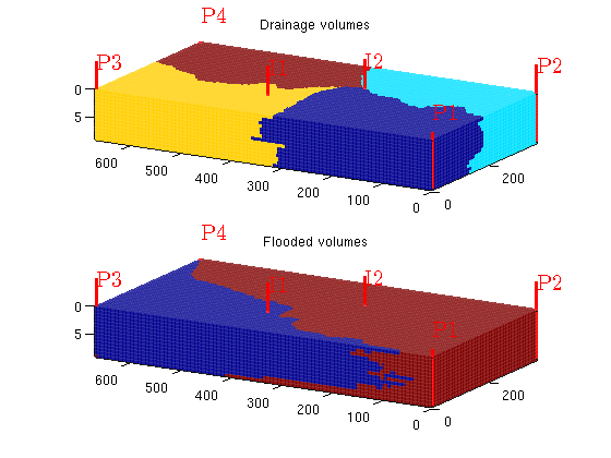
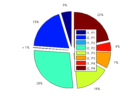
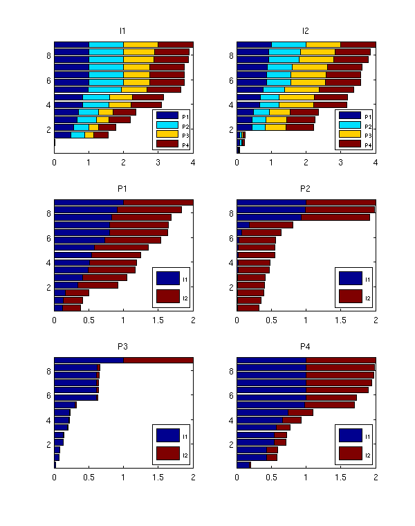
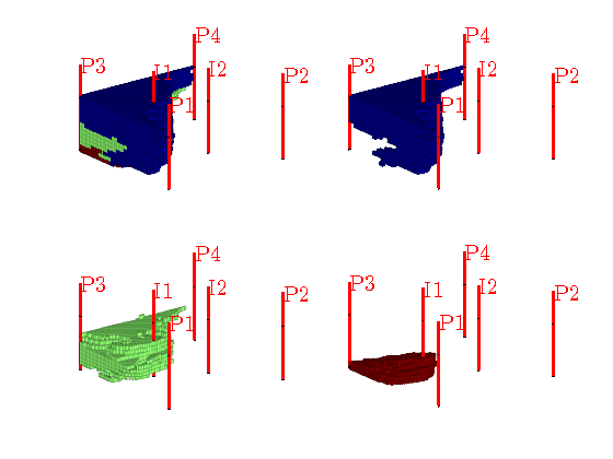
Well-pair diagnostics

In this example, we show how one can use static tracer partition to visualize drainage and flooded volumes and compute well-pair diagnostics such as volumes

Contents

Set up problem

As our example, we consider a subsample of Model 2 from the 10th SPE Comparative Solution Project, but with a different well pattern

mrstModule add spe10

cartDims = [  60,  220,  15];
physDims = [1200, 2200, 2*cartDims(end)] .* ft();   % ft -> m
wtype    = {'bhp', 'bhp', 'bhp', 'bhp', 'bhp', 'bhp'};
wtarget  = [200,   200,   200,   200,   500,   500  ] .* barsa();
wrad     = [0.125, 0.125, 0.125, 0.125, 0.125, 0.125] .* meter;
wloc     = [  1,   60,     1,   60,  20, 40;
              1,    1,   220,  220, 130, 90];
wname    = {'P1', 'P2', 'P3', 'P4', 'I1', 'I2'};

if ~readCache({cartDims}, 'verbose', false),
   rock = SPE10_rock(1:cartDims(end));
   rock.perm = convertFrom(rock.perm, milli*darcy);
   rock.poro = max(rock.poro, 1e-4);
   G  = cartGrid(cartDims, physDims);
   G  = computeGeometry(G);

   writeCache({cartDims}, {'G', 'rock'});
end
W = [];
for w = 1 : numel(wtype),
   W = verticalWell(W, G, rock, wloc(1,w), wloc(2,w), 1 : cartDims(end), ...
                    'Type', wtype{w}, 'Val', wtarget(w), ...
                    'Radius', wrad(w), 'Name', wname{w});
end
fluid = initSingleFluid('mu', 1*centi*poise, 'rho', 1014*kilogram/meter^3);

Drainage and flooded volumes

rS = initState(G, W, 0);
T  = computeTrans(G, rock);
rS = incompTPFA(rS, G, T, fluid, 'wells', W);
D = computeTOFandTracer(rS, G, rock, 'wells', W);

clf, subplot(2,1,1);
plotCellData(G,D.ppart,'EdgeColor','w','EdgeAlpha',.05);
axis tight; plotWell(G,W); title('Drainage volumes');
set(gca,'dataaspect',[1 1 0.1]), view(-60,15)

subplot(2,1,2);
plotCellData(G,D.ipart,'EdgeColor','w','EdgeAlpha',.05);
axis tight; plotWell(G,W); title('Flooded volumes');
set(gca,'dataaspect',[1 1 0.1]), view(-60,15)

Volumes for each well pair

figure
WP = computeWellPairs(rS, G, rock, W, D);
pie(WP.vols, ones(size(WP.vols)))
legend(WP.pairs,'location','Best');

Allocation factors for well pairs

We show a bar plot of well allocation factors for each completion of the wells as a function of the depth of the completion. The allocation factor is defined as the normalized, cummulative flux in/out of a well from bottom and up.

figure; set(gcf,'Position',[10 70 600 760]);
for i=1:numel(D.inj)
   subplot(3,2,i)
   alloc = bsxfun(@rdivide,cumsum(WP.inj(i).alloc,1),sum(WP.inj(i).alloc));
   barh(WP.inj(i).z, alloc,'stacked'); axis tight
   lh=legend(W(D.prod).name,4);
   set(lh,'units','pixels'); lp = get(lh,'OuterPosition');
   set(lh, 'FontSize',6, 'OuterPosition',[lp(1:2)+[lp(3)-60 0] 60 60]);
   title(W(D.inj(i)).name);
end
for i=1:numel(D.prod)
   subplot(3,2,i+numel(D.inj))
   alloc = bsxfun(@rdivide,cumsum(WP.prod(i).alloc,1),sum(WP.prod(i).alloc));
   barh(WP.prod(i).z, alloc,'stacked'); axis tight
   lh=legend(W(D.inj).name,4);
   set(lh,'units','pixels'); lp = get(lh,'OuterPosition');
   set(lh, 'FontSize',6, 'OuterPosition',[lp(1:2)+[lp(3)-60 0] 60 60]);
   title(W(D.prod(i)).name);
end

Look at individual completions

To llok more closely at the performance of the different completions along the well path, we can divide the completion intervals into bins and assign a corresponding set of pseudo wells for which we recompute flow diagnostics. As an example, we split the completions of I1 into three bins and the completions of I2 into four bins.

[rSp,Wp] = expandWellCompletions(rS,W,[5, 3; 6, 4]);
Dp = computeTOFandTracer(rSp, G, rock, 'wells', Wp);

Display flooded regions for I1

figure,
subplot(2,2,1);
plotCellData(G,Dp.ipart, Dp.ipart<4,'EdgeColor','w','EdgeAlpha',.05);
view(3), plotWell(G,W,'radius',3); axis tight off;
for i=1:3
   subplot(2,2,i+1)
   plotCellData(G,Dp.ipart, Dp.ipart==i,'EdgeColor','w','EdgeAlpha',.05);
   view(3), plotWell(G,W,'radius',3); axis tight off; caxis([1 3]);
end

Display flooded regions for I2

figure
for i=1:4
   subplot(2,2,i)
   plotCellData(G,Dp.ipart, Dp.ipart==i+3,'EdgeColor','w','EdgeAlpha',.05);
   view(3), plotWell(G,W,'radius',3); axis tight off; caxis([4 7]);
end

Published December 20, 2012