In this example we illustrate how allocation factors for well pairs can be used to assess the quality of upscaling. As our example, we consider a subsample of Model 2 from the 10th SPE Comparative Solution Project, but with a different well pattern consisting of two central injectors and producers at each of the four corners.

Contents

Set up fine-scale problem

mrstModule add spe10 coarsegrid
fprintf(1,'Setting up fine-scale problem ...');
cartDims = [  60,  220, 15];
physDims = [1200, 2200, 2*cartDims(end)] .* ft();   % ft -> m
if ~readCache({cartDims}, 'verbose', false),
   rock = SPE10_rock(1:cartDims(end));
   rock.perm = convertFrom(rock.perm, milli*darcy);
   rock.poro = max(rock.poro, 1e-4);
   G  = cartGrid(cartDims, physDims);
   G  = computeGeometry(G);
   writeCache({cartDims}, {'G', 'rock'});
end
wtype    = {'bhp', 'bhp', 'bhp', 'bhp', 'bhp', 'bhp'};
wtarget  = [200,   200,   200,   200,   500,   500  ] .* barsa();
wrad     = [0.125, 0.125, 0.125, 0.125, 0.125, 0.125] .* meter;
wloc     = [  1,   60,     1,   60,  20, 40;
              1,    1,   220,  220, 130, 90];
wname    = {'P1', 'P2', 'P3', 'P4', 'I1', 'I2'};
W = [];
for w = 1 : numel(wtype),
   W = verticalWell(W, G, rock, wloc(1,w), wloc(2,w), 1 : cartDims(end), ...
                    'Type', wtype{w}, 'Val', wtarget(w), ...
                    'Radius', wrad(w), 'Name', wname{w});
end
fluid = initSingleFluid('mu', 1*centi*poise, 'rho', 1014*kilogram/meter^3);
fprintf(1,'done\n');

Setting up fine-scale problem ...done

Solve flow problem and compute flow diagnostics

fprintf(1,'Solving fine-scale problem ...');
mrstModule('add', fullfile(ROOTDIR, 'mex', 'AGMG'))
rS = initState(G, W, 0);
T  = computeTrans(G, rock);
rS = incompTPFA(rS, G, T, fluid, 'wells', W);
D  = computeTOFandTracer(rS, G, rock, 'wells', W);
WP = computeWellPairs(rS, G, rock, W, D);
fprintf(1,'done\n');

Solving fine-scale problem ...done

Upscale petrophysical data

Upscale the permeability using either simple harmonic averaging, which we expect will give quite poor results, or a standard flow-based method from the 'upscaling' module, which is expected to give reasonable results. Notice that the computational cost of the flow-based method may be quite high for large subsets of the SPE10 model. For the porosity, we use a simple average.

flowbased = true;
fprintf(1,'Upscaling ...');
cfac = [5 5 3];
p  = partitionUI(G, cartDims./cfac);
if flowbased
   mrstModule add upscaling agglom coarsegrid
   CG = generateCoarseGrid(G, p);
   crock.perm = upscalePerm(G, CG, rock, 'Verbose',true);
else
   for i=1:3;
      K = accumarray(p,1./rock.perm(:,i))./accumarray(p,1);
      crock.perm(:,i) = 1./K;
   end
end
crock.poro = accumarray(p, rock.poro)./accumarray(p,1);
fprintf(1,'done\n');

Upscaling ...Computing upscaled permeabilities... Elapsed time is 72.100324 seconds.
done

Setup the coarse-scale problem

fprintf(1,'Setting up coarse-scale problem ...');
Gc  = cartGrid(cartDims./cfac, physDims);
Gc  = computeGeometry(Gc);
cwloc(1,:) = ceil(wloc(1,:)/cfac(1));
cwloc(2,:) = ceil(wloc(2,:)/cfac(2));
Wc = [];
for w = 1 : numel(wtype),
   Wc = verticalWell(Wc, Gc, crock, cwloc(1,w), cwloc(2,w), ...
                     1 : (cartDims(end)/cfac(end)), ...
                    'Type', wtype{w}, 'Val', wtarget(w), ...
                    'Radius', wrad(w), 'Name', wname{w});
end
fprintf(1,'done\n');

Setting up coarse-scale problem ...done

Solve coarse-scale flow problem and compute flow diagnostics

fprintf(1,'Solving coarse-scale problem ...');
rSc = initState(Gc, Wc, 0);
Tc  = computeTrans(Gc, crock);
rSc = incompTPFA(rSc, Gc, Tc, fluid, 'wells', Wc);
Dc  = computeTOFandTracer(rSc, Gc, crock, 'wells', Wc);
WPc = computeWellPairs(rSc, Gc, crock, Wc, Dc);
fprintf(1,'done\n');

Solving coarse-scale problem ...done

Compare allocation factors

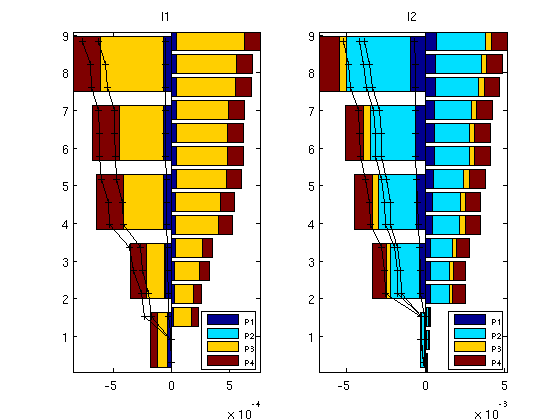
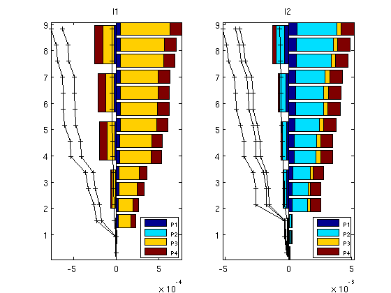
We contrast the allocation factors for the injection wells computed on the fine and the coarse model. Ideally, bars on the negative axis that represent the allocation factors for the coarse model should be the mirror of the bars on the positive axis that represent the allocation factors for the fine model. To simplify the comparison, the fine-scale allocation factors are indicated by lines on top of those of the coarse scale. From the figures below, we see that the flow-based method is able to reproduce the allocations with reasonable accuracy, whereas when using the harmonic averaging methods, the estimates are far off (as should be expected).

figure;
for i=1:numel(D.inj)
   subplot(1,2,i)
   barh(WP.inj(i).z, cumsum(WP.inj(i).alloc,1),'stacked');
   lh=legend(W(D.prod).name,4);
   hold on
   barh(WPc.inj(i).z, -cumsum(WPc.inj(i).alloc,1), 'stacked');
   plot(-cumsum(cumsum(WP.inj(i).alloc,1),2), WP.inj(i).z, '+-k');
   hold off, axis tight
   set(lh,'units','pixels'); lp = get(lh,'OuterPosition');
   set(lh, 'FontSize',6, 'OuterPosition',[lp(1:2)+[lp(3)-60 0] 60 60]);
   title(W(D.inj(i)).name);
end

Flow-based upscaling	Harmonic upscaling

Published with MATLAB® 7.13