MRSTlogo_web_banner_light_thinner_Epi.png

Flow diagnostics
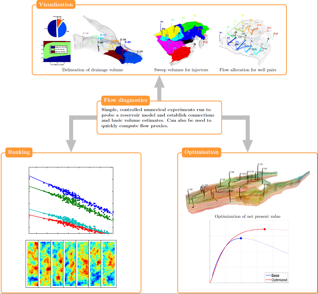
The term ’flow diagnostics’ as used herein, refers to a set of simple and controlled numerical flow experiments that are run to probe a reservoir model, establish connections and basic volume estimates, and quickly provide a qualitative picture of the flow patterns in the reservoir. The methods can also be used to compute quantitative information about the recovery process in settings somewhat simpler than what would be encountered in an actual field, or be used to perform what-if and sensitivity analyzes in parameter regions surrounding preexisting simulations. As such, these methods offer a computationally inexpensive alternative to performing full-featured multiphase simulations to rank, compare, and validate reservoir models, upscaling procedures, and production scenarios.

Basic quantities

Flow diagnostics are constructed based on a (single-phase) pressure solution and can be used as efficient tools for assessing flow patterns and well allocation factors. The 'diagnostics' module in MRST offers a computationally inexpensive alternative to performing full-featured multiphase simulations in order to rank, compare, and validate reservoir models and production scenarios.

The basic diagnostic routine computes the following information:

  • Time-of-flight denotes the time it takes an imaginary, neutral particle to travel from the nearest injector to a given point in the reservoir. Time-of-flight from all injectors define natural time lines in the reservoir. Likewise, one can define the reverse time-of-flight as the travel time from a given point and to the nearest production well. The sum of the two time-of-flights gives the total residence time of the corresponding flow path.
  • Stationary tracer distributions from each injection and production well.  For each injector we conduct an artificial tracer test by setting the concentration to unity in that well and to zero in all other injectors. The stationary tracer distribution reveals the regions in the reservoir that are influenced by the injector. For producers, similar tracer tests are conducted by reversing the flux field. Tracer partitions can also easily be computed for individual well completions.
  • Tracer partitions for injectors and produces obtained by thresholding the tracer distributions. From these partitions, one can easily define drainage volumes, sweep volumes, well-pair connections, well allocation factors, et.

Time-of-flight and tracer partitions are often associated with streamlines, but in the 'diagnostics' module they are computed using a standard first-order, upstream, finite-volume method. This way, these quantities can easily be computed in a robust manner on general unstructured grids. However, the resulting values will not be very representative in a pointwise sense, in particular in cells that contain flow paths with significantly different residence times. More accurate values are obtained if one computes averaged time-of-flight per tracer region.
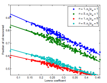
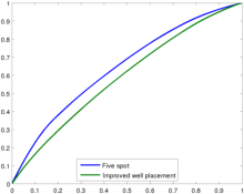
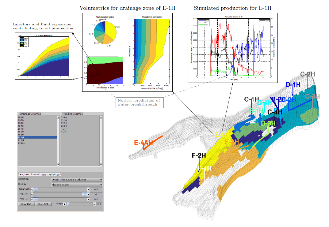
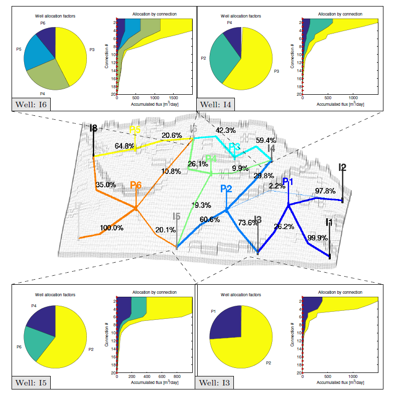
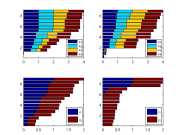
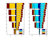
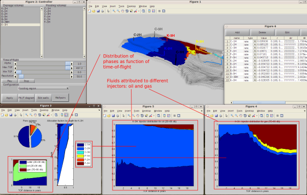

fivespot


Maindiag

allocationfactors


Estimating sweep efficiency

Based on time-of-flight, the module can also compute three quantities that can be used to assess the heterogeneity of a reservoir model:

  • Flow-capacity/storage-capacity F-Phi diagrams. Making an analogue to 1D  displacement theory, the F-Phi curve is the equivalent to a plot of the fractional flow versus saturation. For a homogeneous displacement, this curve will be a straight line Phi=F.
  • Sweep efficiency versus dimensionless time in pore volumes using the F-Phi curve as flux function
  • Lorenz coefficient is a popular measure of heterogeneity. It is equal to twice the area under the F-Phi curve and above the F=Phi line. Values vary between 0 for a homogeneous displacement to 1 for an infinitely heterogeneous displacement.

The upper figure shows how the Lorenz coefficient can be used to predict the oil recovery for different permeability and well configurations. The oil recovery simulated for four different fluid models is plotted as a function of the Lorenz coefficient for all the 85 horizontal layers in Model 2 from the SPE 10 Comparative Solution Project.

The lower figure shows flow and storage capacity diagram for two different well configurations. The blue line represents the F-Phi curve of a standard five-spot well configuration. The green line shows the F-Phi curve of an alternative well placement that has been obtained by rigorous mathematical optimization with the Lorenz coefficient as objective function. Because the green curve lies much closer to a linear curve corresponding to an ideal linear displacement, one can expect the optimized well placement to give significantly higher recovery, which was also confirmed by a full simulation.


Volumetric connections and flow patterns

The most obvious use of tracer partitions and time-of- flight values is to use these cell-based values as a basis to provide improved visualization of flow patterns. Drainage and sweep volumes can be defined using a majority vote over tracer concentrations so that each cell is assigned to a speci c injector or producer. Communication between wells is obtained by intersecting drainage and swept volumes, and the resulting volume partition can be used to identify the pore volume associated with each well pair, or to compute well allocation factors, i.e., the fraction of the producer's inflow that can be attributed to a given indicator. A very intuitive visualization of the evolution of injected fluids is obtained by combining swept volumes with the forward time-of-flight.

The upper plot shows the sweep volumes associated with a single injector delineated and colorized by injector-producer connections. The lower plot shows pore volumes assigned to each producer (left) and the allocation factors per depth (right), which makes it easy to estimate influences between well pairs.

In MRST, all these ideas are combined in an interactive viewer that makes it easy to look at allocation factors, drainage/flood volumes for well pairs and so on for specific regions of time-of-flight. Because the flow diagnostics is so quick to compute, the user may use these measures to interactively adjustment well positions and rates, experiment with adding new infill wells, etc. Likewise, a simple preview of future production can be obtained by visualizing the fluid distribution inside the drainage volume of a given producer as function of the reverse time-of-flight.


Examples

The two figures below exemplify how flow diagnostics can be used to pre-process and post-process more comprehensive multiphase simulations to gain better insight into flow patterns and volumetric connections in a reservoir model

 
Postprocessing for a black-oil simulation of the Norne field with focus on producer E-1H. The upper-left plot shows the instant fluid distribution as a function of travel time from the producer, the upper-middle plot shows the instant volumetrics inside the drainage zone (right-lower plot), where the upper-right plot shows the well response over the full simulation history.   Pre-processing to determine volumetric connections: Well pairs in communication shown as solid lines, colored by producer and percentage refering to flux allocation. Pie charts show total rate allocation for each well, whereas the graphs show cumulative rate allocation for individual well completions.


Literature

  1. O. Møyner, S. Krogstad, and K.-A. Lie. The application of flow diagnostics for reservoir management. SPE J., Vol. 20, No. 2, pp. 306-323, 2015. DOI: 10.2118/171557-PA
  2. User Guide to Flow Diagnostics in MRST - Flow Diagnostics Preprocessors for Model Ensembles. hdl.handle.net/11250/2687239
  3. User Guide to Flow Diagnostics Postprocessing - Simulations in MRST and ECLIPSE Output Format. hdl.handle.net/11250/2687032
  4. F. Watson, S. Krogstad, K.-A. Lie. Flow diagnostics for model ensembles. ECMOR XVII - 17th European Conference on the Mathematics of Oil Recovery, 2020. DOI: 10.3997/2214-4609.202035133
  5. S. Krogstad and H.M. Nilsen. Efficient adjoint-based well-placement optimization using flow diagnostics proxies. ECMOR XVII - 17th European Conference on the Mathematics of Oil Recovery, 2020. DOI: 10.3997/2214-4609.202035227.
  6. M. Borregales, O. Møyner, S. Krogstad, K.-A. Lie. Data-driven models based on flow diagnostics. ECMOR XVII - 17th European Conference on the Mathematics of Oil Recovery, 2020. DOI: 10.3997/2214-4609.202035122
  7. K.-A. Lie, S. Krogstad, O. Møyner. Application of flow diagnostics and multiscale methods for reservoir management. 2015 Reservoir Simulation Symposium, Houston, Texas, USA, 23-25 February 2015. DOI: 10.2118/173306-MS
  8. A. F. Rasmussen and K.-A. Lie. Discretization of flow diagnostics on stratigraphic and unstructured grids. ECMOR XIV, Catania, Sicily, Italy, 8-11 September 2014. DOI: 10.3997/2214-4609.20141844
  9. J. R. Natvig and K.-A. Lie. Fast computation of multiphase flow in porous media by implicit discontinuous Galerkin schemes with optimal ordering of elements. J. Comput. Phys, Vol. 227, Issue 24, pp. 10108-10124, 2008. Doi:  10.1016/j.jcp.2008.08.024.
  10. B. Eikemo, K.-A. Lie, H.K. Dahle, and G.T. Eigestad. A discontinuous Galerkin method for transport in fractured media using unstructured triangular grids. Adv. Water Resour. Vol. 32, Issue 4, pp. 493-506. 2009. Doi: 10.1016/j.advwatres.2008.12.010.
  11. J. R. Natvig, K.-A. Lie, B. Eikemo, and I. Berre. An efficient discontinuous Galerkin method for advective transport in porous media. Adv. Water Resour, Vol. 30, Issue 12, pp. 2424-2438, 2007. Doi: 10.1016/j.advwatres.2007.05.015
  12. M. Shahvali, B. Mallison, K. Wei, and H. Gross. An alternative to streamlines for flow diagnostics on structured and unstructured grids. SPE Journal, Vol. 17, No.  3, September 2012, pp. 768-778. Doi: 10.2118/146446-PA
  13. G. M. Shook and K. M. Mitchell. A robust measure of heterogenity for ranking earth models: the F Phi curve and dynamics Lorenz coefficient. Paper SPE 124625. SPE Annual Technical Conference and Exhibition, New Orleans, 4-7 October, 2009. Doi: 10.2118/12465-MS.

Download

This module is included with MRST from version 2012b and onwards under the name 'diagnostics'.

Published October 1, 2012

Examples of various uses of flow diagnostics. Enlarge the picture

Tutorial: compute time-of-flight and stationary tracer as well as three different measures for heterogeneity. Read more..


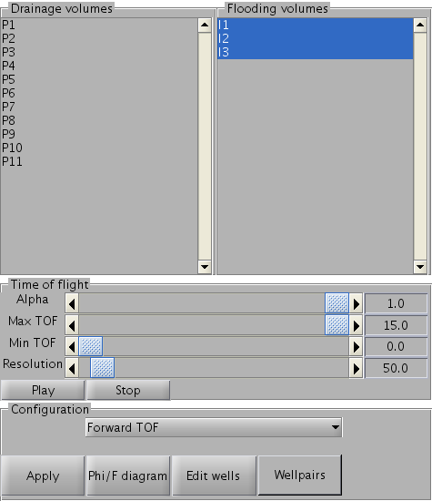
Tutorial: visualize drainage and flooded volumes and compute well-pair diagnostics. Read more..


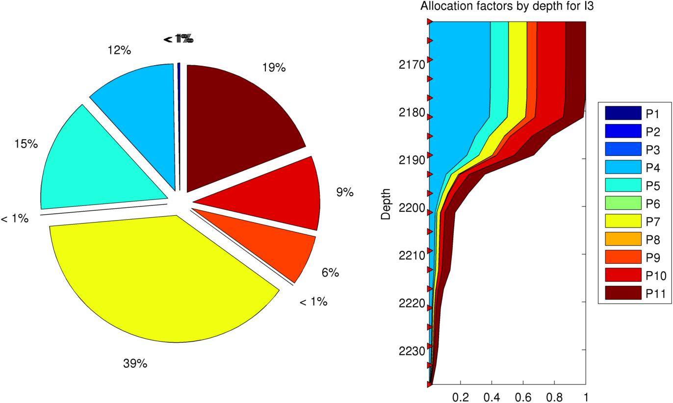
Tutorial: use well-allocation factors to assess the quality of upscaling. Read more..


Tutorial: use SAIGUP geomodel realization to set up a simulation model and then launche the interactive diagnostics tool. Read more..


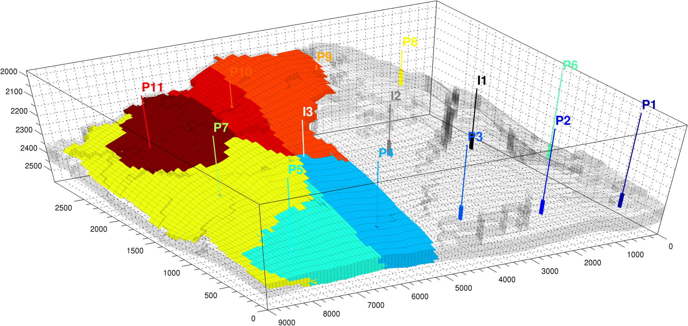
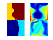
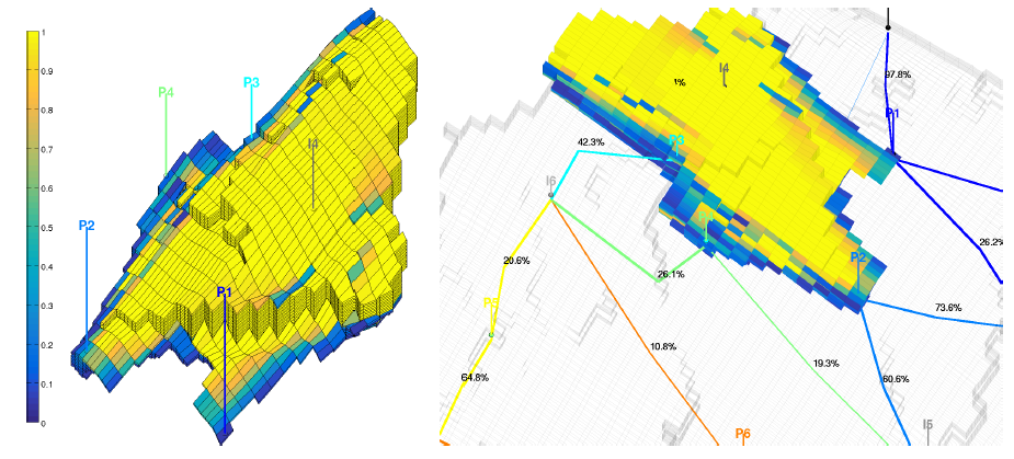
Example of injection tracer region superimposed on a well-allocation map for the SAIGUP data set. Click to enlarge..


Release video from MRST 2013a

Youtube video demonstrating interactive visualization and flow diagnostics in MRST.