Simulate long term migration on the Utsira formation

This example demonstrates simulation of long-term migration of CO₂ in the Utsira formation using incompressible flow and Dirichlet pressure boundary conditions. CO₂ is injected in the cell nearest to the Sleipner field where CO₂ injection is ongoing.

mrstModule add gridtools mex

Set up fluid properties and hydrostatic pressure

We define approximate hydrostatic pressure for a set of z values to use as initial values:

$P = P_0 + rho_{water}\cdot \delta h g_z$

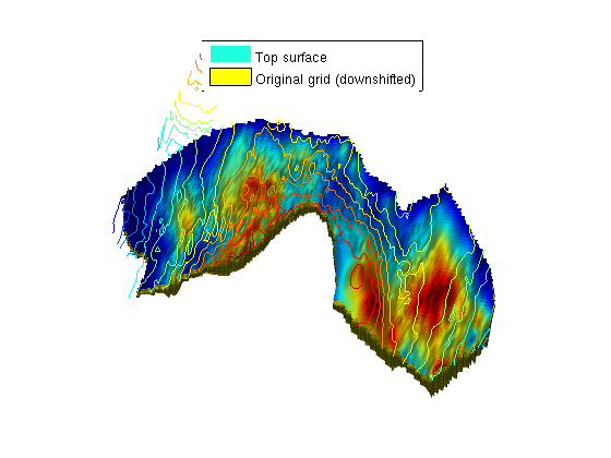
At the same time, we define the physical properties of CO₂ and water at our reference pressure.

We also define a coarsening of the full Utsira grid. The full grid contains a fairly large number of cells, so we coarse by a factor 3. This can be changed to a higher or lower number depending on the available processing power and the patience of the user.

muw = 0.30860;  rhow = 975.86; sw    = 0.1;
muc = 0.056641; rhoc = 686.54; srco2 = 0.2;
kwm = [0.2142 0.85];

mu  = [muc  muw ] .* centi*poise;
rho = [rhoc rhow] .* kilogram/meter^3;

% Define reservoar top
topPos = 300*meter;
topPressure = 300*barsa;

% Turn on gravity
gravity on;
grav = gravity();

% Pressure function
pressure = @(z) topPressure + rho(2)*(z - topPos)*grav(3);

% Default viewing angle
v = [-80, 80];

% Coarsening factor
nc = 3;

Set up injection parameters

We inject a yearly amount of 1 Mt/year (which is approximately the same as the current injection at Sleipner) for a period of 100 years, followed by 4900 years of migration. During injection the timesteps are smaller than during migration.

T_tot = 5000*year;
T_inj =  100*year;

N = 20;
dT_inj  = T_inj / N;  % short time steps during injection
dT_long = dT_inj*5;   % longer steps during migration

% ~ 1Mt annual injection
rate = 1e9*kilogram/(year*rhoc*kilogram*meter^3);

% Approximate position of the Sleipner field
sleipnerPos = [438514, 6472100];

Set up a grid corresponding to the Utsira formation

The Sleipner field has a history of CO₂ injection. It is embedded in the Utsira formation. We will demonstrate how the larger formation grids can be used to simulate long term migration.

[grids, info, petrodata] = getAtlasGrid('Utsirafm', 'nz', 5, 'coarsening', nc);

% Store heightmap data for contour plots
info = info(cellfun(@(x) strcmpi(x.variant, 'top'), info));
info = info{1};

G = processGRDECL(grids{1});

% Depending on the coarsening factor, occasionally very small subsets of
% cells may become disconnected. We guard against this by taking only the
% first grid returned by processGRDECL,  which is guaranteed by
% processGRDECL to be the one with the most cells.
G = G(1);
try
    % Try accelerated geometry calculations.
    G = mcomputeGeometry(G);
catch ex %#ok
    % Fall back to pure MATLAB code.
    G = computeGeometry(G);
end

[Gt, G] = topSurfaceGrid(G);

Plot grid along with top surface

We downshift the full grid to plot it alongside with the top surface. We also add a simple light to show the surface variation in height, which highlights regions where structural trapping is possible.

To show the relation to the original dataset, we plot contour lines on the original height data. Note that as the final grid is the intersection between the provided height and thickness datasets, some contour lines do not correspond to any part of the grid.

figure;
Gplot = G;
Gplot.nodes.coords(:,3) = Gplot.nodes.coords(:,3) + 100;
plotCellData(Gt, Gt.cells.H)
plotGrid(Gplot, 'edgea', .1)
light
lighting phong
view(v);
legend({'Top surface', 'Original grid (downshifted)'}, 'Location', 'North')
contourAtlas(info, 15, 1)
axis tight off

Set up rock properties and compute transmissibilities

We use the averaged values for porosity and permeability as given in the Atlas tables. Since cellwise data is not present, we assume to averaged values to be valid everywhere.

pd = petrodata{1};
rock.poro = repmat(pd.avgporo, G.cells.num, 1);
rock.perm = repmat(pd.avgperm, G.cells.num, 1);
rock2D    = averageRock(rock, Gt);
T = computeTrans(Gt, rock2D);
T = T.*Gt.cells.H(gridCellNo(Gt));

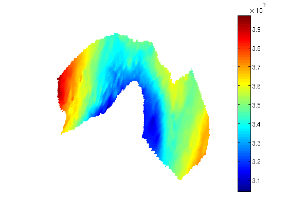
Set up fluid

fluid = initSimpleVEFluid_s('mu' , mu , 'rho', rho, ...
                                'height'  , Gt.cells.H,...
                                'sr', [srco2, sw],'kwm',kwm);

Set up well and boundary conditions

This example is using an incompressible model for both rock and fluid. If we assume no-flow on the boundary, this will result in zero flow from a single injection well. However, this can be compensated if we use the physical understanding of the problem to set appropriate boundary conditions: The Utsira formation is enormous compared to the volume of the injected CO₂. Thus, it is impossible that the injection will change the composition of the formation significantly. We therefore assume that the boundary conditions can be set equal to hydrostatic pressure to drive flow.

% Find the cell nearest to the Sleipner field
si = findEnclosingCell(Gt, sleipnerPos);

% Add an injector well for the CO₂
W = addWell([], G, rock, si,...
   'Type', 'rate', 'Val', rate, 'comp_i', [1,0], 'name', 'Sleipner field');

% Add pressure boundary
bnd = boundaryFaces(Gt);
bc = addBC([], bnd, 'pressure', pressure(Gt.faces.z(bnd)), 'sat', [0 1]);

% Convert to 2D wells
W2D = convertwellsVE_s(W, G, Gt, rock2D,'ip_tpf');

Set up initial reservoir conditions

The initial pressure is set to hydrostatic pressure. Setup and plot.

sol = initResSolVE_s(Gt, pressure(Gt.cells.z), 0);
sol.wellSol = initWellSol(W2D, 0);

clf;
plotCellData(Gt, sol.pressure);
view(v); axis tight off; colorbar

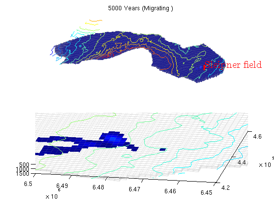
Run the simulation

Solve for all timesteps, and plot the results at each timestep.

t = 0;
dT = dT_inj;
tt = ' (Injecting)';
while t < T_tot;
    if t >= T_inj
        W2D = [];
        dT  = dT_long;
        tt  = ' (Migrating )';
    end
    sol = incompTPFA(sol, Gt, T,       fluid, 'wells', W2D, 'bc', bc);
    sol = implicitTransport(sol, Gt, dT, rock2D, fluid, 'wells', W2D, 'bc', bc, 'Verbose', true);
    t = t + dT;

    % Plotting
    [s h] = normalizeValuesVE(Gt, sol, fluid);

    % Plot the whole formation
    subplot(2,1,1)
    cla
    plotCellData(G, s, 'edgec', 'k', 'edgea', .1, 'edgec', [.6 .6 .6]);
    plotWell(G, W); caxis([0 .9]);
    contourAtlas(info)
    title([formatTimeRange(t) tt])
    axis tight off
    view(v);

    % Plot the area around the Sleipner formation
    subplot(2,1,2)
    cla
    plotCellData(G, s, s > 1e-3);
    contourAtlas(info,25)
    plotGrid(G, 'facec', 'none', 'edgec', [.6 .6 .6], 'edgea', .1)
    axis([4.2e5 4.6e5 6.45e6 6.5e6]), caxis([0 .9]);
    view(v);

    drawnow
end

Published February 12, 2013

Contents